Telecommunication Fraud Detection Using Data Mining techniques

(1)

UNIVERSITY OF

P

ORTO

FACULTY OF

ENGINEERING

Telecommunication Fraud Detection

Using Data Mining techniques

João Vitor Cepêda de Sousa

F

OR

J

URY

E

VALUATION

Master in Electrical and Computers Engineering

Supervisor: Prof. Dr. Carlos Manuel Milheiro de Oliveira Pinto Soares Co-Supervisor: Prof. Dr. Luís Fernando Rainho Alves Torgo

(2)

c

(3)

Abstract

This document presents the final report of the thesis “Telecommunication Fraud Detection Using Data Mining Techniques”, were a study is made over the effect of the unbalanced data, generated by the Telecommunications Industry, in the construction and performance of classifiers that allows the detection and prevention of frauds. In this subject, an unbalanced data set is characterized by an uneven class distribution where the amount of fraudulent instances (positive) is substantially smaller than the amount normal instances (negative). This will result in a classifier which is most likely to classify data has belonging to the normal class then to the fraud class. At first, an overall inspection is made over the data characteristics and the Naive Bayes model, which is the classifier selected to do the anomaly detection on these experiments. After the characteristics are presented, a feature engineering stage is done with the intent to extend the information contained in the data creating a depper relation with the data itself and model characteristics. A previously proposed solution that consists on undersampling the most abundant class (normal) before building the model, is presented and tested. In the end, the new proposals are presented. The first proposal is to study the effects of changing the intrinsic class distribution parameter in the Naive Bayes model and evaluate its performance. The second proposal consists in estimating margin values that when applied to the model output, attempt to bring more positive instances from previous negative classification. All of these suggested models are validated over amonte-carloexperiment, using data with and without the engineered features.

(4)

(5)

Acknowledgements

My first words of acknowledgment must be to my mother and my baby momma, for the patient they had and the support they gave me.

I would also like to thank my supervisor and co-supervisor for all the help and advisement they gave me during this work, and all the patient that they showed when I ask my thousands of silly questions.

To finish, I also like to thank my friend for the support and my laptop for not shutting down and don’t giving up on my thousand hours data processing marathons!

João Cepêda

(6)

(7)

“Prediction is very difficult, especially if it’s about the future.”

Niels Bohr

(8)

(9)

List of Figures

2.1 Blue Box Device . . . 7

2.2 2013 WorldWide Telecommunications Fraud Methods Statistics. . . 8

2.3 Outliers example in a bidimensional data set. . . 9

2.4 2 models ROC curve Comparison . . . 13

3.1 First proposal model construction squematics . . . 25

3.2 Second proposal model construction squematics . . . 26

4.1 Class distribution in each day . . . 32

4.2 Number of calls per hour in each day . . . 32

4.3 Number of calls by duration in each day . . . 33

4.4 Real scenario simulation system . . . 35

4.5 Normal Naive Bayes Model . . . 36

4.6 Undersample Naive Bayes Model . . . 36

4.7 Priori Naive Bayes Model . . . 36

4.8 After-Model Naive Bayes Model (Proposed Solution) . . . 37

4.9 Normal Naive Bayes Model Without Signature . . . 38

4.10 Undersample Naive Bayes Model Without Signature . . . 39

4.11 Normal Naive Bayes Model With Signature 1 . . . 39

4.12 Undersample Naive Bayes Model With Signature 1 . . . 40

4.13 Normal Naive Bayes Model With Signature 2 . . . 40

4.14 Undersample Naive Bayes Model With Signature 2 . . . 41

4.15 Undersample Naive Bayes Model Without Signature For The First 10% Under-Sample Percentage . . . 42

4.16 Undersample Naive Bayes Model With Signature 1 For The First 10% Under-Sample Percentage . . . 42

4.17 Undersample Naive Bayes Model With Signature 2 For The First 10% Under-Sample Percentage . . . 43

4.18 Priori Naive Bayes Model Without Signature . . . 43

4.19 Priori Naive Bayes Model With Signature 1 . . . 44

4.20 Priori Naive Bayes Model With Signature 2 . . . 44

4.21 After-Model Naive Bayes Model With Signature 0 . . . 45

4.24 Normal Naive Bayes Model ROC Curve . . . 47

4.25 After-Model Naive Bayes Model ROC Curve . . . 47

(12)

(13)

List of Tables

1.1 Annual Global Telecommunications Industry Lost Revenue . . . 1

2.1 Frequency-Digit correspondence on the Operator MF Pulsing . . . 6

4.1 Amount of converted positive intances and their corresponding label. . . 46

(14)

(15)

Abbreviations

ASPeCT Advanced Security for Personal Communications Technologies CDR Call Details Record

CFCA Communications Fraud Control Association CRISP-DM Cross Industry Standard Process for Data Mining DC-1 Detector Constructor

LDA Latent Dirichlet Allocation MF Multiple-Frequencies SMS Short Message System SOM Self-Organizing Maps SVM Support Vector Machine

(16)

(17)

Chapter 1

Introduction

1.1

Motivation

Fraud is a major concern in the telecommunications industry. This problem results mainly in dam-ages in the financial field [1] since fraudsters are currently "leaching" the revenue of the operators who offer these type of services [2,3]. The main definition of telecommunication fraud correspond to the abusive usage of an operator infrastructure, this means, a third party is using the resources of a carrier (telecommunications company) without the intention of paying them. Others aspects of the problem that causes a lower revenue, are fraud of methods that use the identity of legitimate clients in order to commit fraud, resulting in those clients being framed for a fraud attack that they didn’t commit. This will result in client’s loss of confidence in their carrier, giving them reasons to leave. Besides being victims of fraud, some clients just don’t like to be attached to a carrier who has been victim of fraud attacks and since the offering of the same services is available by multiple carriers, the client can always switch very easily between them [4].

2005 2008 2011 2013 Estimated Global Revenue (USD) 1.2 Trilion 1.7 Trilion 2.1 Trilion 2.2 Trilion

Lost Revenue to Fraud (USD) 61.3 Bilion 60.1 Bilion 40.1 Bilion 46.3 Bilion % Representativa 5.11% 3.54% 1.88%

Table 1.1: Annual Global Telecommunications Industry Lost Revenue

Observing the table1.1it is possible to verify the dimension of the "financial hole" generated by fraud in the telecommunications industry and the impact of fraud in the annual revenue of the operators.

There are a couple of reasons which make the fraud in this area appealing for some fraudsters. One is the difficulty in the location tracking process of the fraudster, this is very expensive process and requires a lot of time, which make it impractical if trying to detect a large amount of indi-viduals. Another reason is the technological requirements to commit fraud in these systems. A fraudster doesn’t require a particularly sophisticated equipment in order to practice fraud in this systems [5].

(18)

2 Introduction

All these evidences generate the need to detect the fraudsters in the most effective way in order to avoid future damage to the telecommunications industry.

Data mining techniques are suggested has the most valuable solution, since it allows to identify fraudulent activity with certain degree of confidence. It also works specially well in great amounts of data, a characteristic of the data generated by the telecommunications companies.

1.2

Problem

Telecommunication operators store large amounts of data related with the activity of their clients. In these records exists both normal and fraudulent activity records. It is expected for the fraudulent activity records to be substantially smaller than the normal activity. If it were the other way around this type of business would be impractical due to the amount of revenue lost.

The problem that arises when trying to effectively detect fraudulent behaviour in this field is due to the class distribution (normal or fraud) in the data used to construct the classifier (model that allows the classification of data as normal or fraudulent). More precisely, when a classifier is built using unbalanced class data then it is most likely to classify each instance belonging to the class with more evidences, this being the normal class.

When evaluating the performance of the classifier, it is required to know precisely the objective of the operator in order to achieve the maximum performance. Usually, the main objective of an operator is to reduce the cost of the fraudulent activity on the revenue.

It is then required to associate a cost to the classification results, this means that the misclassi-fication of fraudulent and normal activity should have associated costs given by the operator. Then it is only required to adjust the classifier in order to minimize that cost. Some operators might like to detect all the fraudulent activity even if that results in a lot of misclassified normal activity. This can be obtained by associating a large cost to a misclassified fraudulent instance so that the amount of missed frauds is quite small.

1.3

Objectives

The objective of this dissertation is to study the performance of the Naive Bayes classifier in the anomaly prediction using unbalanced class data sets and discuss possible adaptations to the model in order to counter the unbalanced class effect.

Summarizing, the main objectives of this project are:

1. Evaluate the performance of the Naive Bayes classifier on unbalanced data sets; 2. Apply existing adaptation to the model and evaluate the performance improvements; 3. Propose new solution to this problem;

(19)

1.4 Document Structure 3

1.4

Document Structure

The present document is divided into 5 chapters: Introduction, State of the Art, Naive Bayes, Study Case and Conclusion. In the introduction, the motivation and objectives for this work are presented as well as the problem definition. In the State of the Art, a recap is made in previously studies in the area of Telecommunications fraud, Anomaly detection and Data Mining. In the Naive Bayes chapter, is presents the standard Naive Bayes model, the extensions, the adaptions and the proposed modifications. In the Case Study chapter, is presented the data, the feature engineering, the methodology, the results and the discussion. In the final chapter, the conclusion, it is made an overall overview over the objectives and the future work.

(20)

(21)

Chapter 2

State Of the Art

2.1

Telecommunications Fraud

Fraud is commonly described as the intent of misleading others in order of obtaining personal benefits [3]. In the telecommunications area, fraud is characterized by the abusive usage of and carrier services without the intention of paying. In this scenario there might emerge two victims:

• Carrier— Since there are resources of the carrier that are being used by a fraudster, it

exists a direct loss of operability since those resources could be used on a legit client. This will also result in the loss of revenue since these usage will not be charged;

• Client— When victim of a fraud attack, the client integrity is going to be contested in order

to detect if this is really a fraud scenario. If the client is truly the victim, then the false alarm will compromise the confidence that the client erstwhile had in the carrier. Still some clients might even be charged for the services that the fraudster used, therefore destroying even further the confidence of the client on the carrier;

The practice of fraud is usually related to money, but there are some other reasons like political motivations, personal achievements and self-preservation that make the fraudsters motivated in committing the attacks[3] .

2.1.1 History of Fraud

Since the beginning of commercial telecommunications, the fraudsters have been causing financial damage to the companies who offered these services [6]. At the start, the carriers didn’t have the dimension, or the users, that they have nowadays and so the amount of fraud cases wasn’t as big. This could mean that the financial damage caused, wasn’t as high as it is today, but this isn’t actually true. Indeed the amount of frauds was smaller but, the cost associated with a fraud attack in the beginning infrastructure was further big that it is nowadays. Later on and due to the technological advances, the cost of a fraud attack to the carrier has been decreasing, but on the

(22)

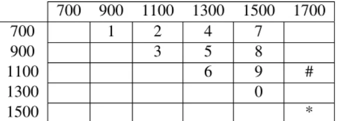
6 State Of the Art 700 900 1100 1300 1500 1700 700 1 2 4 7 900 3 5 8 1100 6 9 # 1300 0 1500 *

Table 2.1: Frequency-Digit correspondence on the Operator MF Pulsing

opposite direction, the amount of occurrences have been increasing creating a constant financial damage [3].

An interesting story about one of the first type of telecommunication fraud happened in 1957, in the telephony network of AT&T. At this time AT&T was installing their firsts automatic PBX’s fromThe Bell Systemscompany. To access the control options of the network (e.g. call routing), the operators would send MF sound signals in 2400Hz band directly to the telephony line, were all the other calls signalling were passing. Since the control signals could be sent from any point of the network, this allowed users to ear and therefore try to copy those signals. The fraud on the telephone lines were the user copied those control signals in order to use the network resources, like free calling, was denominated byphreaking(phone + freak). The pioneer in this type of fraud was Joe Engressia, also known asJoybubbles. He figured that, by whistling to the microphone in headset of his phone at the right frequency he could establish a call between two users without being charged. Later on another phreaker, John Darper, realized that the whistle offered, at the time, in the cereal boxCaptain Crunch, was able to produce a perfect sound signal at the frequency required to access the control commands of the network. This discovery gave him the nickname ofCpt. Crunch.

In the 60s The Bell Systemsreleased the paper were the control signal were described [7]. This paper and the previous discoveries made from John Darper and Joe Engressia, allowed for Steve Wozniak and Steve Jobs (yes, the creators of apple) to create a device that allowed the job of freaking to become much easier. The device was namedBlue Box, and it was a simple box with a keypad and a speaker that would connect to the microphone on the telephone headset. By pressing a key, the device emitted the correspondent sound signal trough the speaker and therefore into the network allowing to access the control with the previous correct frequency whistling effort. The key to MF conversion is visible in table 2.1. All these discoveries and the invention of the blue box had a purely academic purpose, but this didn’t discouraged other people to copy the device and abuse its purpose.

More recently, the telecommunications fraud concerns extended to another all new dimension since the commercialization of the internet and to a whole new pack of services. New types of fraud appeared and less control over the users the operators has. This resulted in an increased difficulty in preventing the problem. Carriers keep investing in new security systems in order to prevent and fight the fraudsters, but the fraudsters don’t give up and keep trying to find new ways to bypass those securities. This might results in new types of fraud besides the ones that the security

(23)

2.1 Telecommunications Fraud 7

Figure 2.1: Blue Box Device

systems could prevent. It is safe to say that there is everlasting fight between the carriers and the fraudsters. The operators try to avoid their systems from being attacked and the fraudsters trying to detect and abuse weaknesses on the systems [3].

2.1.2 Fraud Methods

Telecommunications is wide area because it is composed by a variety of services like internet, telephones, VOIP etc... Fraud in this area is consequently an extensive subject. There are types of frauds that are characteristic of one service, like the SIM cloning fraud which is particular to the mobile phone service and there are frauds that cover a bunch of services like the subscription fraud, which is associated to the subscription of services. Next, it will be described the fraud methods that are considered the most worrying.

• Superimposed Fraud— This kind of fraud happens when the fraudster gains unauthorized

access to a client account. In telecommunications, this includes the SIM card cloning fraud that consists in the copy of the information inside the SIM card of the legitimate client to another card in order to use it and access the carrier services. This mean that the fraudster superimposes the client actions pretending to be that person. Despite this fraud method not being so common lately, it is the fraud who has been most reported in his overall existence, and because of that, the fraud that has been most for studies [8];

• Subscription Fraud— This fraud occurs when a client subscribes to a service (e.g.

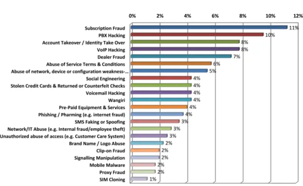
in-ternet) and use it without the intention of paying. This is the fraud method who have been more reported in the year of 2013 (see fig.2.2) [3];

• Technical Fraud— This fraud occurs when a fraudster exploits the technical weaknesses

of a telecommunications system for his benefit. These weaknesses are usually discovered by the fraudster in a trial and error methodology or by the direct guidance of an employee who is committing internal fraud. Technical fraud in mostly common on newly deployed

(24)

8 State Of the Art

Figure 2.2: 2013 WorldWide Telecommunications Fraud Methods Statistics.

services, where the chance of existing an error of development is bigger. Some of this error are only fixed after the deployment of the system and in some cases after the fraud has been committed. This fraud includes the very know, “system hacking” [3];

• Internal Fraud — Happens when an employee of a telecommunications company uses

internal information about the system in order to exploit it for personal or others benefit. This fraud is usually related with other types of fraud (e.g. technical fraud);

• Social Engineering — Instead of trying to discover the weaknesses of a carrier system

(like the trial and error system of technical fraud), the fraudster uses his soft skills in order to obtain detailed information about the system. These information’s can be obtained from the employees of the carrier with them knowing the fraudster true intentions. In a special case, there might even exist a relation between this method and the internal fraud where the fraudster convinces one employee in committing the fraud in his name [3];

Figure2.2displat the fraud methods with more incidences in the year 2013 worldwide.

2.2

Anomaly Detection

Anomaly detection, is one of the areas of the application of data mining and consists in techniques of data analysis that allow detection patterns of likelihood in a data set and then defines patterns of data that are consider normal or abnormal. An anomaly (or outlier) is an instance of data that doesn’t belong to any pattern predefined as normal or in fact belong to a pattern consider

(25)

2.2 Anomaly Detection 9 2 N 1 N 1 o 1 O Y X

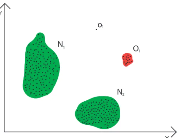
Figure 2.3: Outliers example in a bidimensional data set.

abnormal [9]. In summary, the instances belonging to the pattern consider normal are considered normal and those who don’t belong are considered abnormal. If those patterns are well defined at an early stage and the model used to do the anomaly detection is well built, this process can also be used in the prediction (prevention) of anomalies. Some example of anomaly detection fields are:

• Fraud detection - telecommunications fraud, credit card fraud or insurances fraud;

• Intrusion Detection — network intrusion detection, live house security systems;

• Network Diagnoses — network monitoring, network debugging;

• Image Analyses — image processing;

• Failure Detection — networks failure prediction;

The process used to build an anomaly detection model is composed by two stage the training stage and the test stage. The first stage is the training stage and is used to build the model used for detection. The second stage is the training stage and is used to evaluate the performance of the model [10]. For each of this stage a data set must be divided in two portions one for training and other for testing. These portions are usually 70% and 30% of the original data set for training and testing respectively.

In a visual analysis, the anomaly detection of a small set of data wouldn’t be complicated. The problem appears when the amount of data grows exponentially, and the visual analysis starts to be less precise. In the figure2.3we can observe two patterns of data in the group N1e N2, one smaller

group O1and an instance o1. In the case of anomaly detection, the instance o1is undoubtedly and

outlier, and the groups N1e N2are not outliers, but the smaller group O1can be either a group of

(26)

10 State Of the Art

2.2.1 Anomaly Types

When building an anomaly detection system, it is necessary to specify the type of anomaly that the system is able to detect [9]. This anomalies can be of the type:

• Point Anomalies— When an individual instance is considered abnormal to the rest of the

data, then this anomaly is a point anomaly. This is the most basic type of anomaly. In the figure2.3the sample o1is considered a point anomaly. An example of a point anomaly in

the telecommunications context is when a client that has a mean call cost of valueX and suddenly a call of valueY is made (Y » X). Then due to the difference from the mean, the call of costY is very likely to be a point anomaly;

• Contextual Anomalies— In this case, a data instance is considered an anomaly only if

differs from the rest of the data given a certain context (or scenario). The same instance can be classified as normal given a different context. The context definition is defined when formalizing the data mining problem. An example of contextual anomaly in the telecom-munications context is when we compare the number of calls made by a user within the business context against personal context. Is most likely for a client to make less calls in the personal context then the business context. So if an extraordinary big number of calls appear for that client, it will be considered abnormal in the personal context and normal in the business context;

• Collective Anomalies — A group of related data that is considered anomalous according

to the rest of the data set, is called a collective anomaly. Individual instances in that group may not be considered anomalies when compared to the rest of the data, but when joined together they are considered an anomaly. An example of collective anomaly in the telecom-munications context is when the monitoring system that counts the number of active calls in the infrastructure per second is displaying 0 active calls for a 1 minute period measure. This means that 60 measures were made and all of them were returning 0. A minute without any active calls is very likely to be considered and anomaly, but if we take each one of those 60 measures as a single case, or even smaller groups, then they might be considered normal; 2.2.2 Data Mining

Data mining is a process that allows the extraction of non-explicit knowledge from a data set [11]. This process is very useful when handling big amounts of data, which is a characteristic of the data generated from the telecommunications companies. A typical data mining problem starts from the need to find extra information from an existing set of data. Each step in the conventional process is measured in order to achieve the maximum amount of information for the planned objective. The steps that compose the standard process are:

• Data cleaning and integration — In the integration, data from multiple sources is

com-bined. Cleaning consist in the removal of noise and data that are consider redundant and useless.

(27)

2.2 Anomaly Detection 11

• Data Selection and Transformation— In the selection, only the data that is relevant for

the task is selected. This data is prepared for the model used in the data mining process (next step). Besides the data selection the transformation allows the creation of new data derived from the previous data.

• Data Mining— This is the step where the new knowledge will be extracted from the data.

Some models used in this step are described in the anomaly detection chapter;

• Evaluation— In this step the output of the data mining process (previous step) is evaluated.

The performance of the model is measured and the results are evaluated from the objective point of view;

• Knowledge Presentation— Presentation of the results to the user. This presentation

de-pends of the desire output, it can be a visual presentation like data charts or a tables or it can be another data set that can be used as the input for a new data mining process;

Despite presenting a well-defined order, it doesn’t necessarily mean that to achieve a good result we are only required to execute only once each one of these steps. In most cases a good result only appears when some of the steps and thoroughly repeated [12].

2.2.3 Learning Types

When building a model for an anomaly detection process, it is required to know if the data that is being used to construct the model has any identification regarding the objective variable [9]. The objective variable is the variable that, in the case of anomaly detection data mining, says to which class does given data instance belong to (normal or anomalous). This is also known as the label. The learning type differs regarding the labelling is on the input data. The existent learning types are:

• Supervised— In the supervised anomaly detection, the data used to construct the model

has labels of normal and abnormal data. This type of learning is very useful for prediction models because exists information about both classes;

• Semi-Supervised— In the semi-supervised anomaly detection, the data used to construct

the model has only labels in the instances regarding one of the classes, usually the normal class. Models using this type of learning usually try to define the labelled class properties. Any instances that doesn’t fit in those properties is label in the opposite class;

• Unsupervised— In unsupervised anomaly detection, there is no information labelling of

the instances. This type of learning is mostly used in clustering models because they don’t require any previous information about the labelling, they just group data using the likeli-hood of the information.

(28)

12 State Of the Art

Sometimes the labelling process is made by hand of an analyst. This is a tiring job and due to this, sometimes the amount of labelled data is very tiny. In some cases there might be bad labelling of the data [13].

2.2.4 Model Evaluation

2.2.4.1 Evaluation Metrics

One of the most important steps when building an anomaly detection model, is evaluating its performance. In the case of anomaly detection, to evaluate the performance it is required for the data to be already labelled in order to compare the resulting labels with the original ones, therefore supervised anomaly detection. In the fraud detection subject, the output of the model is a binary variable which mean, that the model is supposed to evaluate each instance as anomaly or not (in this case fraud or not). This introduces the concept of positive and negative class. The positive class is the one that the model is targeting, in this case the anomaly, and the negative class is the other class, the normal. The basic indicator of performance is the amount of:

• True Positive— Positive class instances classified as positive (anomalous instance labelled

as anomalous);

• True Negative— Negative class instances classified as negative (normal instance labelled

as normal);

• False Positive— Negative class instances classified as positive (normal instance labelled as

anomalous);

• False Negative — Positive class instances classified as negative (anomalous instance

la-belled as normal);

This allows the calculation of more descriptive measures like therecallandprecision, which are the most popular performance indicators for binary classification.Recallis the fraction of the original positive class instances that were classified as positive and theprecisionas the fraction of resulting positive class instance that were well classified.

precision= T P

T P+FP (2.1)

recall= T P

T P+FN (2.2)

2.2.4.2 ROC

Another interesting approach to describe the model performance is the ROC curve. To plot a ROC curve it is required for the model to output a probability or ranking of the positive class [12]. In the case of binary classification, is usually the probability for a given instance to belong to

(29)

2.2 Anomaly Detection 13 0.00 0.25 0.50 0.75 1.00 0.00 0.25 0.50 0.75 1.00

False Positive Rate

T rue P ositiv e Rate Curves: ROC1 ROC2

Figure 2.4: 2 models ROC curve Comparison

the positive class. The same assumption can be made when the output is in the form of scores, which is the positive class score of each instance. This curve plots the relation between the True Positive Rate (TPR)(or recall) and the False Positive Rate (FPR) when the boundary of decision changes. The boundary of decision is the threshold used to transform the ranking or probability into a class label. The method to draw the curve is then to make the decision boundary to go from the minimum value in the output probability to the maximum value and in each step measure the TPR and FPR. truepositiverate=T P P = T P T P+FN=recall (2.3) f alsepositiverate=FP N = FP T N+FP (2.4)

Chart2.4presentes the comparison between 2 ROC curves. Both curves are drawn above the dotted line(X=Y) which means that the TPR is always bigger than the FPR for every value that the decision boundary get. This also means that they are both good models to classify the used data. This ROC comparison also displays the perfect model which is represented by theROC1curve. In the perfect model, all the positive instances have 100% positive probability generated by the model.

2.2.4.3 Model Validation

Model validation techniques focus in repeating the model construction and validation stages in different testing and training data and in each experiment, observe the performance indicators.

(30)

14 State Of the Art

There are a couple of methods to make the selection of the data used in the train and test stage like the holdout method, k-fold cross-validation, bootstrap, monte-carlo experiment... In this document it is only described 2 of these methods: the k-fold cross-validation and the monte-carlo experiment. In the k-fold cross-validation, the data set is randomly divided into k subsets of the same size with similar initial characteristics (e.g. same class distribution as the original data set), this subsets are also known asfolds. In each interaction onefoldis used for training and, individually, the remainingfoldsare used for testing. The same fold is never used as training and testing at the same time. The method ends when everyfoldwas used as training and testing [12]. When k = 1 this method is called "leave-one-out" cross-validation.

In the monte-carlo experiment, the original data set is partitionedMtimes into disjoint train and test subsets. The train and test data sets are fractions of size nt and nv, respectively, of the

original data set. The main feature of this validation method is that, despite the train and test data sets being randomly generated, they respect the temporal order of the data, therefore the train data set is generated from randomly selecting data that is on a time interval "before" the data used for the generation of the test data set. This method is especially important for validating time series forecasting models [14].

2.3

Data Mining Techniques for Anomaly Detection

Data mining is mainly used to extract further knowledge from a data set, but in this case the results that the data mining process produce can be further used to detect anomalies. In this case, the outputs of this process are usually presented in two ways:

• Labels — each instance of data that is submitted to anomaly detection gets a labels has

being positive or negative (anomalous or normal);

• Scores— each instance of data gets a value, created by a scoring technique, that represents

thedegreeof anomaly also known asanomaly score. This allows the results to be ranked and give priority anomalies with higher scores;

Next, it will be presented some of the existing techniques that use data mining processes for anomaly detection.

2.3.1 Clustering based techniques

Clustering is a process that has the objective of joining data that have similar characteristics. These groups are called clusters. Anomaly detection using clusters is made by applying a clustering algorithm to the data and afterwards, the classification of the data is made by one of the following principles:

• Normal data instances belong to a cluster and abnormal instances don’t— In this case

the clustering algorithm shouldn’t force every instance to belong to a cluster, because if it does it won’t appear any outlier which result in no abnormal instances;

(31)

2.3 Data Mining Techniques for Anomaly Detection 15

• Normal data instances are closer to clusters centroid and abnormal instances are far

— The cluster centroid is the graphical centre of the cluster. The distance must be measured according the same graphical characteristics;

• Normal data instances belong to denser clusters and abnormal instances are in less

denser clusters— In this case it is requires to measure the density of each cluster of data.

To define the density value where a cluster belongs to each one of the classes it is required to define a threshold values;

These techniques don’t require the data to be labelled, therefore unsupervised learning. They also work with several types of data. Clustering allows the retrieval of more useful information which might not been available at a first glance at the data. Although the anomaly detection is fast and simple after the cluster have been achieved, the clustering process is very slow and computational expensive. The performance of the anomaly detection process depends mostly on the clustering process, bad clusters mean bad detection [9].

2.3.2 Nearest neighbour based techniques

Nearest neighbours techniques require measure that characterizes the distance between data in-stances, also known as similarity. This technique differs from clustering because it requires the analysis of the distance between each instance of the data without the need to group them (clus-ter). Clustering techniques might also use the same principle in the clustering algorithm but they create cluster as output, and this technique doesn’t. The distance calculation is made by a relation between the attributes of the data in both instances and it differs from the data format. Techniques based on nearest neighbour can be of two types:

• Kthnearest neighbour techniques— This techniques starts by giving each data instance

an anomaly score that is obtained by evaluation of the distance to its kth neighbours. Af-terwards the most usual way to separate anomalous instances from normal instances is by applying a threshold to the anomaly scores calculated previously;

• Relative density techniques— In this technique each instance evaluated by measuring the

density of its neighbourhood. The neighbourhood density is measured by the amount of in-stance which diin-stance measure a range value previously defined. Anomalous data inin-stances have less dense neighbourhoods and normal data instance have more dense neighbourhoods; These techniques can use unsupervised learning, which makes the model construction only guided by the rest of the data features. In this case, if the normal instances don’t have enough neighbours and the anomalous instances do, the model will fail to correctly label the anomalous instances. This techniques have best performance under semi-supervised learning, because the anomalous instances have less probability to create a neighbourhood therefore they become more easily targetable. This also becomes a problem if the normal instances don’t have enough neigh-bours, increasing the probability of the anomalous labelling. Since the key aspect of this technique

(32)

16 State Of the Art

is the distance parameter, it allows the adaption of the model to other type of data only requiring to change the way the distance is calculated. This is also the main downside, because bad distances calculation methods will result in poor performance [9].

2.3.3 Statistics Techniques

In statistics techniques the anomaly detection is done by evaluating the statistical probability of a given instance to be anomalous. Therefore the first step in these techniques is the construction of a statistical model (usually for normal behaviour) that fits the given data. The probability of an instance to be anomalous is them derived from the model. In the case that the model represents the normal behaviour probability, when a data instance is evaluated in the model, the ones that output high probability are considered normal and the ones that output low probability are considers anomalous. The probability construction models can be of the type:

• Parametric— Statistical models of these type assume its probabilistic distribution is

de-fined by a group of parameters which are derived from the given data. This allows the model to be defined piori of the data analysis. An example of a parametric probability distribution is the Gaussian distribution that is defined by parameters of mean (µ) and standard deviation (σ).

• Non-parametric— This models requires a further analysis in the data, because they can’t

be defined trough a group of parameters achieved from the data. This makes the model much more precise because fewer assumptions are made about the data. An example of model of this type are the histogram based models, in which the histogram is built using the given data.

These techniques outputs scores, therefore allowing to relate that score with a confidence interval. In the modelling stage, if result is proven to be good, then this model is able to work under an unsupervised method. The downside of this technique is that works under the assumption that the probabilities are distributed under a specific way for a parametric scenario which doesn’t actually stand for a true evidence is most cases, especially for larger scale data sets [9].

2.3.4 Classification Techniques

Anomaly detection using classification techniques require the construction of a classifier. A clas-sifier is a model constructed under supervised learning which stores intrinsically properties of the data, and afterward, will be able to classify data instances as normal or anomalous. Summariz-ing, the classifier construction process, in the classification techniques is composed by 2 stages: the learning stage where the classifier (model) is built and the testing stage where the classifier is tested. The normal instances that the classifier is able to classify can be of two types:

• Uni-class— Normal instances belong to only one class;

(33)

2.3 Data Mining Techniques for Anomaly Detection 17

There are several approaches for the classification techniques, the main difference between them are the classifier type (model) that each one builds and use. Some of these approaches are:

• Neural Networks— In this approach during the training stage, a neural network is trained

with data from the normal class (uni-class or multi-class). After the model is build, during the test, data instances are used as input of the network. If the network accepts that instance then it shall be classified as normal, if not it should be classified as anomalous;

• Bayes networks— In this approach the training stage is used to obtain the priori probability

regarding the each one of the classes. In the testing stage, the classification is made by calculating the posterior probability (the Bayes theorem) of every class in each data instance. The class with higher probability for that instance, represents the class which that instance is going to be labelled with;

• SVM— In this approach the training stage is used to delimit the region (boundary) where data is classified as normal. In the testing stage, the instances are compared to that region, if they fall in the delimited region they are classified as normal, if not, as anomalous;

• Rules– In this approach, the training stage is used to create a bunch of rules (e.g. if else

conditions) that characterize the normal behaviour of the data. In the testing stage, every instance is evaluated with those rules, if they pass every condition they are classified as normal, if not, as anomalous;

These techniques use very powerful and flexible algorithms and they are also rather fast, be-cause it is only required to apply the classifier to each instance. The downside is that the supervised learning require a very effective labelling process, and if it has any mistakes it will later result in a lack of performance of the classifier. The output of this technique is in most of the cases a class label, which hardens the process of scoring [9].

2.3.5 Unbalanced Data Set

An unbalanced data set, is a data set where the amount of existing classes is not balanced. This means that the amount of instances belonging to one of classes is much more abundant than the other. In the case of anomaly detection is quite usual for the amount of anomaly instances to be quite smaller than the amount of normal ones. This is a problem because it will make the anomaly detection model detect very easily the normal data but very hardly the anomalies. A solution to counter this effect is by changing the model construction in order to generate conditions to nullify the unbalanced class effect, but in fact this solution is not one of the most famous because it requires greater research and changes on the standard model construction which should be seen as a black box [15]. Therefore some optional solutions appear that assume that the model is actually a black box, and these solutions are:

(34)

18 State Of the Art

• Under-sample the most abundant class— before constructing the model, remove some

of the most abundant class instances (with sampling techniques). This might result in lack of information for the most abundant class conditions but the model will be class balanced;

• Over-sample the less abundant class— before constructing the model, repeat some of the

less abundant class instances. This might result in some overflowing information regarding the less abundant class, because some of the information of thatclass will appear repeated; Some extra solutions worth mention, focus around feature engineering in order to give the data self-conditions in the given context in order to counter the unbalanced effect [16].

2.4

Data Mining on Fraud Detection

Most works of data mining done in telecommunications fraud detection have the objective of de-tecting or preventing the methods of superimposed fraud [8][13] and subscription [1][17], because these are the fraud methods that have done more damage to the telecommunications industry.

2.4.1 Data Format

Projects done in fraud telecommunications aren’t always easy to begin, because the telecommuni-cations companies can’t allow third parties direct access to data of their clients due to agreements between carrier and the clients. The kind of data that is mostly used to do this studies are the so called CDR, call details records (or call data records)[6,2,1,5,13,17,18]. This records have a log like format and they are created every time that the client finish using a service of the operator. The format of the records may change from company to company but the most common attributes are:

• Caller and called Identification Number;

• Date and time;

• Type of Service (Voice Call, SMS, etc...) ;

• Duration;

• Network access point identifiers;

• Others;

This data doesn’t actually compromise the identification or the content that was switched be-tween the users, therefore it doesn’t violate any privacy agreement. If some logs do compromise the true identification of the clients the data can be anonymize by the company before being re-leased.

(35)

2.4 Data Mining on Fraud Detection 19

2.4.2 User Profiling

In most techniques of fraud detection studies, the authors choose to use techniques of user profiling in order to describe the behaviour of the users [19,6,5,2]. User profiling is done by separating the data that has anything to do with a user and develop a model that represent its behaviour. This allows to insert extract additional information from the data used, and even add some additional information to the data set, like new attributes, before doing the model for anomaly detection.

The user models can be optimized by giving an adaptive characteristic to the profile of the user [8]. This means that the user model must be updated every time the user makes an interaction with the system. Users don’t have linear behaviour their models shouldn’t also be linear.

Profiling requires a lot of information about the users in order to build the most representative behaviour model. The CDR, are very useful to create the behaviour models, however to make a more realistic representation of the user, it would be requires more information about him, which is rather difficult due to confidentiality agreements.

2.4.3 Rule based applications

The authors [8], presented a method for superimposed fraud detection based on rules. They used a group of adaptive rules to obtain indicators of fraudulent behaviour from the data. These indicators were used for the construction of monitors. The monitors define fraudulent behaviour profiles and are used as input for the analysis model, also known asdetector[19]. The detector combines all the several monitors with the data generated along the day by a user, and outputs high confidence alarms of fraudulent activity.

The author [18] developed a system for fraud detection in new generation networks. The system is composed by two modules: one for interpretation and other for detection. In the model of interpretation, the CDR’s raw data is used as an input, and the module analysis and convert that data into CDR objects, which will be used to feed the classification module. In the classification model, the CDR objects will be subject to a series of filter analysis. The filters are actually rule based classification techniques which rules and correspondent thresholds were obtain previously from real fraudulent data. If a CDR object doesn’t respect the rules in those filters an alarmed is generated. As a result the author said that the model only classifies as false-positive 4% of the data.

2.4.4 Neural networks Applications

In the system for fraud detection built by the author [20], three anomaly detection techniques are used: supervised learning neural networks, parametric statistics techniques and Bayesian net-works. The supervised neural network, is used to construct a discriminative function between the class fraud and non-fraud using only summary statistics. In the parametric statistic technique, the density estimation is generated using a Gaussian mixture model, and it is used to model the past behaviour of every user in order to detect any abnormal change from the past behaviour. The Bayesian networks are used to define the probabilistic models of a particular user and different

(36)

20 State Of the Art

fraud scenarios, this allowing the detection of fraud given a user’s behaviour. This system had a precision of 100% and a recall of 85%.

2.4.5 Other Applications

Another example of an application that uses both techniques (Rules and neural Networks) is the system developed by the authors [1] for the prevision of subscription fraud. This system is com-posed by two modules: the classification module and the prediction model. The classification module, uses a fuzzy rules approach with a tree structure to classify the users past behaviour into one of these classes:subscription fraudulent,otherwise fraudulent,insolventandnormal. The pre-diction module is a multilayer perceptron neural network, that is used to predict if an application for a new phone line correspond to a fraud or not.

The system developed by [17] for telecommunications subscription fraud was composed by 3 stages: pre-processing, clustering and classification. In the pre-processing stage, the raw data was cleaned, prepared and the dimension reduced using a principal components analysis (PCA). In the clustering stage, the data was clustered into homogeneous clusters by the two clustering algorithmsSOMandk-means. If the resulting clusters are very specific, very different from other clusters or outlier clusters (one instance cluster), then they are discarded and they are not used in the classification stage. This stage was also used to insert some new features to the data in order to keep the clusters properties. In the last stage, the classification stage, the instances are classified using the classifiers SVM, neural networks and decision trees. The classifiers are also constructed in several ways: bagging,boosting,stacking,votingandstandard. In the end of the classification process the classifiers performance is compared and the classification is done according the best result.

A very interesting work was done by [21], they experimented visual techniques data mining in order to detect anomalies. They affirm that these techniques offer one great advantage on the contrary of the computational algorithms, because the systems for the human visualization have better dynamism and adaptability therefore having a natural evolution on fraudulent behaviour. These methodology is based in the quality of graphical presentation of the data for posterior human analysis.

(37)

Chapter 3

Naive Bayes

3.1

Algorithm

Naive Bayes is a supervised learning classification algorithm that applies the Bayes theorem with an assumption of independency between the data features [22]. This assumption is what make him naive. The basic Naive Bayes equation is

P(θ|X) =

P(θ)∗P(X|θ)

P(X) (3.1)

where X = { x1,x2,x3, ...,xn}isthedatainstance(groupo f f eatureso f thatinstance), θ is the

class (positive or negative), P(θ |X) is the posterior probability or the probability of a given

instanceX to belong to the class theta, P(θ) is the prior class probability distribution,P(X |θ)

is the prior attribute probability t, andP(X) is the evidence or instance probability. TheNaive characteristics of this algorithm is visible on the numerator. Before applying the independency, the numerator can be re-written using the conditional chain rule

P(θ)∗P(X|θ) =P(θ)∗P(x1,x2,x3, ...,xn|θ)

=P(θ)∗P(x1|θ)∗P(x2,x3, ...,xn|θ,x1)

=P(θ)∗P(x1|θ)∗P(x2|θ,x1)∗P(x3, ...,xn|θ,x1,x2)

(3.2)

∏

i=1 P(xi|θ) (3.3) 21

(38)

22 Naive Bayes

Each of prior attribute probabilities are calculated by the following equation

P(xt |θ) =

Nt,xt,θ

∑j∈xtNj,xt,θ

(3.4) WhereNis the amount of instances with the attributetof valuext belonging to classθ [23].

The denominator, is constant for each instance and results from the sum of the numerator value for all possible output classes in the classification process.

P(X) = m

∑

j=1 {P(θj)∗ n

∏

i=1 P(xi|θj))} (3.5)

Finally, the initial Naive Bayes equation, can be re-written as

P(θ |x1,x2,x3, ...,xn) = P(θ)∗∏n1P(xi|θ) m ∑ j=1 {P(θj)∗ n ∏ i=1 P(xi|θj))} (3.6)

3.1.1 Naive Bayes in Label Classification

If the objective of the Naive Bayes algorithm is to simply classify instances with a label non re-garding the class probability (or ranking) for each instance, then the classification process doesn’t require to know the value of the denominator P(x1,x2,x3, ...,xn) since it is a constant for each

instance. The classification process only requires the result of the numeratorP(θ)∗∏n1P(xi|θ).

This characteristic allows the use of Maximum A Posteriori (MAP) to estimate the valuesP(θ)

and∏n1P(xi|θ)to determine which classθ does a given instanceX achieves its maximum value

[22]. The resulting classification rule is

θ=argmaxθP(θ)∗ n

∏

i=1 P(xi|θ) (3.7) 3.1.2 La Place Correction

When constructing the Naive Bayes model, namely calculating the priori (P(θ)) probability, there

might be some cases where the data doesn’t offer the necessary information regarding a given featurext with a certain valueKfor one of the classesθr, resulting in a prior attribute probability

of value zero. This will later result in an posterior probability for a given instance with the feature xt with valueKto be zero for the classθr, therefore the model will never classify an instance with

that particular characteristic as belonging to any other class even if the rest of the features strongly point for that instance to belong to another class. To avoid this effect, it is usual to use a method calledLaplace Correctionin order to avoid lacks of information. This method simply change the

(39)

3.2 Adaptations 23

initial value of the count for instances with that characteristic in a given class [24]. The formula for a the prior attribute probability calculation for a given attributext on a given classθis

P(xt |θ) =

I+Nt,xt,θ

(K∗I) +∑j∈xtNj,xt,θ

(3.8) whereIis the Laplace Correction value (usually 1) andKis the different values that attribute xt can have.

3.1.3 Continuous Variables

Some attributes in the data set might have continues values, this will cause a problem in the likeli-hood probabilities because it is rather impossible to cover all the values in an interval of continuous values. In order to describe this variables there are some procedures that can be made in order to summarize this variables. One option is to discretize the variable. In this case the continuous variable will be converted to discrete values (e.g. convert continuous intervals to discrete vari-ables) thus being compatible with the standard model construction method. Another very popular option to describe the continuous variables is by making the assumption that the variable values are presented according a parametric probability distribution. This requires some intrinsic adap-tions of the Naive Bayes model in order to calculate the likelihood probability using the density distribution function. A popular solution is to use a Gaussian-like distribution. In this case, during training it is only required to calculate the mean (µθ) and standard deviation (σθ) for the

corre-spondent feature in each classθ [25]. During the test, to calculate the likelihood probability it is

only required to use the following method

P(xt |θ) = 1 σθ √ 2π e−(xt−µθ) 2. 2σ_θ2 (3.9)

3.2

Adaptations

Besides the methods ofunder-sampleand oversample one class of the data in order to counter the unbalanced data effect maintaining the model construction as a blackbox, there are adaptations from previous studies that have targeted the model properties in order to counter those effects. A previously study presents a correction to the prior attribute probabilities calculation in order to counter the unbalanced data effect [24]. This solution was studied on the application on the Naive Bayes classifier to text classification. It can actually be applied as a normalization step to the data, enabling the possibility of leaving the classifier as a blackbox. In this particular solution, due to the data structure, the prior attribute probability is calculated by the following equation

P(w|c) = 1+∑d∈Dcnwd

k+∑w0_∑_d_∈_D

Cnw0d

(3.10) Wherenwd is the number of times that wordwappear on documentd, Dc is the collection

(40)

24 Naive Bayes

objective of this author is to normalize the word count in each class in so that the size for each class is the same. To achieve this, the previous variablenwdis transformed in

α∗ nwd

∑w0_∑_d_∈_D

Cnw0d

(3.11) whereαis the normalization constant and defines the amount of smoothing across word counts

in the dictionary. Whenα=1 the resulting equation is something like

P(w|c) =

1+ ∑d∈Dcnwd

∑w0∑d∈_DCnw0d

k+1 (3.12)

This allows to dimension the prior attribute probability in the case of the objective class (or classes) in order boost the posteriori probability calculation for word with those characteristics.

3.3

Proposal

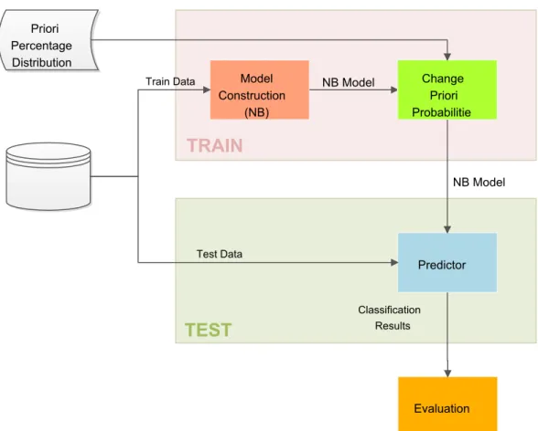
This project proposes the study of two solutions for the anomaly detection system using the Naive Bayes classification algorithm. The first solution consists in studying the impact of changing the prior class probability of the naive Bayes model in the classification process. An representative illustration of the process is presented in figure3.1.

In this first proposal, the only change of the normal process of training and testing of the model is the includedChange Prior Probabilitiesmodule on the training stage. This module changes the values of the p(θ) according to the previously set Prior Percentage Distribution value (PPD). This value determines the values of the negative class prior probability and therefore the value of the positive class prior probability. The method is quite simple

p(θN) =PPD (3.13)

p(θP) =1−PPD=1−p(θN) (3.14)

The second proposal consists in creating some additional features to the model generated by the standard algorithm in order to counter the unbalanced class effect. The process for the model construction and the new features generation are represented in figure3.2.

The main differences from this process for the typical procedure are:

• Train — Instead of simply using the training stage to construct the Naive Bayes model,

after the construction the resulting model will be used to classify (Predictorin the train area of figure3.2) the same data that is used for its construction (train data). The output of that classification process is in the form ofaposterioriprobabilities, in this case, the probabilities for an instance to belong to the positive class or the negative class. Afterwards, the train data and the correspondent aposterioriprobabilities will feed themargin estimator. The margin estimatoris going to derive two new values from that train data and correspondent

(41)

3.3 Proposal 25 Model Construction (NB) Predictor Classification Results

TRAIN

TEST

NB Model NB Model Test Data Train Data Evaluation Change Priori Probabilitie Priori Percentage Distribution

Figure 3.1: First proposal model construction squematics

classification, that will be used in future predictions. These values are denominated as margin values;

• Test — In the testing stage, the model without the new features is going to be used for the prediction as the typical classification process would do. The output of the prediction process also needs to be in the form of class probabilities (like the predictor in the train-ing stage). Instead of ustrain-ing these probabilities to label the test data and finish the process by evaluating the results, the aposterioriprobabilities will feed, together with the previ-ous calculatedmargin valuesinto theapply marginmodule. In this module, theaposteriori probabilities generated by the model are re-calculated using the designed algorithm and the previously calculatedmargin values. This process will results in newaposteriori proba-bilites that will be used to label the data and hand over to the model evaluation stage; The margin values, mn and mp, mentioned previously, are the key aspect of this proposal and they are built upon the following assumption: How can the negative class (most abundant) aposteriori probability be reduced and the positive class (less abundant) aposteriori probability be increased in order to get more True Positives without compromising the True Negatives. The

(42)

26 Naive Bayes Model Construction (NB) Predictor Margin Estimator

Predictor Apply Margin

Classification Results TRAIN TEST Probability Predictions Probability Predictions NB Model Magin Values NB Model Test Data Train Data Evaluation

Figure 3.2: Second proposal model construction squematics

solution is then to study theaposterioriprobabilities for theTrue NegativeandFalse Negativein the classified train data (classified by the model constructed using that same train data) in order to achieve two values that can be applied to the probabilities for both classes in order to obtain better Positive Classification (margin estimator). The margin estimator generates the margin values using the following equation

mn=∑i∈T N(P(θN,i)−0.5) NT N (3.15) mp=∑i∈FN(P(θP,i)−0.5) NFN (3.16)

whereP(θN,i)is theaposterioriprobability of instanceito belong to the negative class (θN),

NT Nis the number of True Negatives,P(θP,i)is theaposterioriprobability of instanceito belong

to the positive class (θP) andNFN is the number of False Negatives. Note that this process occurs

during the training stage, therefore these areaposterioriprobabilities for thetrain data. Also note thatmn, that is themargin valuegenerated from the true negative probabilities, is a positive value while mp, that is themargin value generated from the false negative probabilities, is a negative value.

(43)

3.3 Proposal 27

The previously generatedmargin valuesare used by theapply marginprocess to the test apos-teriorprobabilities using the following equation

Pm(θN,i) =

 



Pprev(θN,i)−mn

(Pprev(θP,i)−mp)+(Pprev(θN,i)−mn) (Pprev(θN,i)−mn)>0

0 (Pprev(θN,i)−mn)<0 (3.17) Pm(θP,i) =    Pprev(θP,i)−mp

(Pprev(θP,i)−mp)+(Pprev(θN,i)−mn) (Pprev(θN,i)−mn)>0

1 (Pprev(θN,i)−mn)<0

(3.18)

where the Pprev(θP,i) andPprev(θN,i) are the aposterior probabilities generated by

classifi-cation process with the naive bayes model and Pm(θP,i) and Pm(θN,i) are the new aposterior

probabilities after applying the margin to the data. Note that the denominator is only a normal-ization process that is applied so thataposterior probabilities keep the property of Pm(θP,i) =

1−Pm(θN,i).

(44)

(45)

Chapter 4

Study Case

4.1

Problem

The problem which this study tries to evaluate, is the performance of classifiers that are built using unbalanced data sets. Classifiers are models that are constructed using labelled data with the intention of hereafter being able to identify (classify) in each instance, by inspecting its attributes, which label, or class, it is most likely to belong to. In this scenario, due to the imbalanced effect which consists on the labelled data having a uneven class distritribution, the classifiers are most likely to classify data instances as belonging to the most abundant class of the data set used for their construction. In these case study, the classification is binary (true of false), therefore there is only a positive and a negative class. Positive being the anomaly and negative the non-anomaly. In the case of this scenarion, the unbalanced data set class distribution can be formalized as

p(θN)>>p(θP) (4.1)

that is, the amount of negative classes is largely bigger then amount of positive classes. This will result in a model (classifier) that classifies instances (X) with similar distributions

p(X|θN)>>p(X|θP) (4.2)

To evaluate this performance the right metrics need to be used, because if we take for instance theaccuracymetric, that calculates the amount of well classified data over the entire population, then these classifiers would have a great performance because they only would need to classify all instances with the most abundant class to achieve a goodaccuracyvalue. The most common metrics used in binary classification are recall andprecision because they describe the correct classified positive instances from the total of Positive instances and from the total of Positive classified instances respectively.

(46)

30 Study Case

4.2

Data

The data set used for this project is composed by two days of CDR (Call Details Records). Each data set has the following features (or attributes):

• DATE • TIME • DURATION • MSISDN • OTHER_MSISDN • CONTRACT_ID • OTHER_CONTRACT_ID • START_CELL_ID • END_CELL_ID • DIRECTION • CALL_TYPE • DESTINATION • VOICEMAIL • DROPPED_CALL

TheDATEis actually the same value in all the instances per data set because, they are already arranged by day and there are two different days, therefore two different values. TIME, as the name suggests, is the time in which the record was made, it is in the format of "HHMMSS" be-ing "HH" hours, "MM" minutes and "SS" seconds. The DURATIONis the amount of time, in seconds, that the service lasted. In the following features some dependencies need to be described because, the called and the caller identification have some feature dependencies in order to know which one is which. In order to formalize this relation, it shall be used the namesuser1anduser2 and further in the description, the relation user - Caller/Called will be defined. MSISDNand

OTHER_MSISDNare than the anonymized (due to legal purposes) cell phone number ofuser1

anduser2respectively.CONTRACT_IDandOTHER_CONTRACT_IDare the number identi-fication of the contract ofuser1anduser2respectively. START_CELL_IDandEND_CELL_ID

are the cell number identifiers where the caller and called, respectively, access the network. The cells are the interfaces for users to the network, in this case this cells are the antennas that commu-nicate with the user cell phones. TheDIRECTIONdescribes the direction of the call, it can take

(47)

4.2 Data 31

two values: "I" for inbound and "O" for outbound. This feature allows to identify the user who made the call and the user who received it, i.e. if theDIRECTIONis "I"(inbound) thenuser1is the caller anduser2is the called user. TheCALL_TYPEis the identifier of the type of the call, or service, which the record corresponds to and it can take the following values: "MO", "ON", "FI", "SV" and "OT". There is no precise description of what those values mean. TheDESTINATION

is a flag-like feature that takes the value "I" for international calls and "L" for local calls. VOICE-MAILis also a flag-like feature that takes the value "Y" for calls who went to voicemail and "N" for calls who didn’t. The last featureDROPPED_CALLis the objective variable for the anomaly detection system and it is also a flag-like feature that take two values: "Y" for a dropped call and "N" for a successful call. Besides the overall description made in the previous paragraph, there are some other characteristics and extra dependencies of the data that should be described:

• Cells identifiers,START_CELL_IDandEND_CELL_ID, don’t seem to be available in every instance. There isn’t a relation in the call characteristics that justifies the missing value because, in some cases, for calls with the same characteristics there are missing values in both IDs or only one ID or even none of them missing. This effect could relate to calls which the users are accessing the networks trough cells who don’t belong to the carrier infrastructure, therefore they can’t be identified;

• Contract identifier ofuser2,OTHER_CONTRACT_ID, in most of the cases doesn’t have any value. This could also relate with the cells identifiers effect explained previously, but in this case is not the infrastructure that belong to another carrier but the client instead;

• All international calls (calls with DESTINATION equal to "I") have theCALL_TYPE

feature always equal to "OT", while in the local calls theCALL_TYPE feature can take values of "MO", "ON", "FI" and "SV";

• All calls who went to voicemail (VOICEMAILhave the value "Y") have theCALL_TYPE

feature equal to "SV" and all have the sameOTHER_MSISDNnumber. This might corre-spond to the anonymized number of the voicemail center;

There are some important characteristics about this data that can be displayed trough some data analysis statistics. The total amount of records used for this project is of 14043142 for the day1data set and 13888323 for theday2data set. The class distribution is visibly unbalanced in the chart4.1whereDay1has about 2.87% dropped calls andDay2about 2.95%.

There are some important characteristic about this data that are required to be presented be-cause, they associate the present data with data that can actually be generated by a true telecommu-nication carrier in a real-world scenario. The first characteristic is presented on chart4.2in which are displayed the amount of calls that are made per hour during each of the days. It is possible to see that the amount of calls that are done between the day time (8am to 9pm) is largely bigger than the amount of calls done during the night time (10pm to 7am) which is the expected distribution. Other aspect is shown on chart4.3were it is displayed the amount of calls done by duration in

(48)

32 Study Case 0.00 0.25 0.50 0.75 1.00 Day1 Day2 Day Class Distr ib ution Label Dropped Normal

Figure 4.1: Class distribution in each day

0 250000 500000 750000 1000000 0 5 10 15 20 Hour Amount of Calls Day Day1 Day2

Figure 4.2: Number of calls per hour in each day

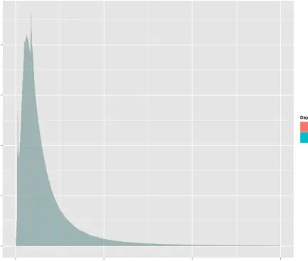
each of the two days. In this case, it is possible to observe that most of the calls are of short dura-tion (< 100 seconds) which is very typical on a real-world scenario. The call duradura-tion presented in this chart (4.3) is only the most relevant duration region, because there are some outlier calls with duration > 5000 seconds which are not represented in this case. One impor