IZA DP No. 1590
International Migration:
A Panel Data Analysis of Economic
and Non-Economic Determinants
Anna Maria Mayda
DISCUSSION P
APER SERIES
Forschungsinstitut zur Zukunft der Arbeit Institute for the Study
International Migration:
A Panel Data Analysis of Economic
and Non-Economic Determinants
Anna Maria Mayda
Georgetown University and IZA Bonn
Discussion Paper No. 1590
May 2005
IZA P.O. Box 7240 53072 Bonn Germany Phone: +49-228-3894-0 Fax: +49-228-3894-180 Email: [email protected]Any opinions expressed here are those of the author(s) and not those of the institute. Research disseminated by IZA may include views on policy, but the institute itself takes no institutional policy positions.
The Institute for the Study of Labor (IZA) in Bonn is a local and virtual international research center and a place of communication between science, politics and business. IZA is an independent nonprofit company supported by Deutsche Post World Net. The center is associated with the University of Bonn and offers a stimulating research environment through its research networks, research support, and visitors and doctoral programs. IZA engages in (i) original and internationally competitive research in all fields of labor economics, (ii) development of policy concepts, and (iii) dissemination of research results and concepts to the interested public.
IZA Discussion Papers often represent preliminary work and are circulated to encourage discussion. Citation of such a paper should account for its provisional character. A revised version may be available directly from the author.
IZA Discussion Paper No. 1590 May 2005
ABSTRACT
International Migration: A Panel Data Analysis of
Economic and Non-Economic Determinants
∗In this paper I empirically investigate economic and non-economic determinants of migration inflows into fourteen OECD countries by country of origin, between 1980 and 1995. The annual panel data set used makes it possible to exploit both the time-series and cross-country variation in immigrant inflows. I focus on both supply and demand determinants of migration patterns and find results broadly consistent with the theoretical predictions of a standard international-migration model. Both first and second moments of the income distribution in the destination and origin countries shape international migration movements. In particular, I find evidence of robust and significant pull effects, that is the positive impact on immigrant inflows of improvements in the mean income opportunities in the host country. Inequality in the origin and destination economies affects the size of migration rates as predicted by Borjas (1987) selection model. Finally, among the non-economic determinants, I investigate the impact on emigration rates of geographical, cultural, and demographic factors as well as the role played by changes in destination countries’ migration policies.
JEL Classification: F22
Keywords: international migration, push and pull factors, network effects
Corresponding author: Anna Maria Mayda
Department of Economics and School of Foreign Service Georgetown University Washington, DC 20057 USA Email: [email protected] ∗
I would like to thank Alberto Alesina, Elhanan Helpman, and Dani Rodrik for support and many insightful comments. For helpful suggestions, I am also grateful to Richard Adams, Marcos Chamon, Bryan Graham, Louise Grogan, Russell Hillberry, Rod Ludema, Maurice Schiff, Tara Watson, Jeffrey Williamson, and participants in the International Workshop at Harvard University, at the 2003 NEUDC Conference at Yale University, at the International Trade Commission Workshop, at the World Bank International Trade Seminar and at IZA Annual Migration Meeting. I am grateful for research assistance provided by Krishna Patel and Pramod Khadka. Finally, I would also like to thank the Center for International Development at Harvard University for making available office space. All errors
1
Introduction
Do flows of international migrants respond to economic incentives, in spite of destination countries’ restrictive immigration policies? Which economic determinants affect international migrationflows? Do non-economic variables - such as geographical, cultural and demographic factors - shape cross-country immigration patterns? What role do host countries’ restrictive
immigration policies play? Are network effects at work? In this paper, I address these
questions using a yearly panel data set that allows me to exploit both the time-series and cross-country variation in international immigrant flows.
Cross-country migration patterns vary considerably over time, and across destination and origin countries (see Appendix 2). Some OECD countries have experienced a decrease
in the size of the annual immigrant inflow between 1980 and 1995.1 Over the same years,
the number of immigrants per year has increased in several other OECD countries.2 The
percentage change of the yearly immigrant inflow in this period ranges between negative 42% (in Japan) and positive 48% (in Canada) (OECD 1997). For all destinations, such changes are anything but monotonic (see Figure 3). The variation in terms of origin countries is remarkable as well.
Both economic and non-economic factors are likely to influence the size, origin, and
destination of labor movements at each point in time and contribute to the variation observed in the data. While clearly it is important to understand the driving forces behind recent international migration patterns, a limited amount of empirical research has been devoted to this topic, perhaps due to past unavailability of cross-country data on migration.
In this paper, I empirically investigate economic and non-economic determinants of bi-lateral immigrant flows, across destination and origin countries.3 Ifirst derive testable pre-dictions about the main factors affecting international migration, using a simple theoretical framework. My model focuses on both supply and demand determinants of immigration patterns. Next, I empirically relate bilateral migrant flows (normalized by origin country’s population) to the economic, geographical, cultural and demographic determinants suggested by the theory. The explanatory variables I identify are mean income opportunities in the source and destination country, their relative income inequality, the distance and common borders between the two countries, their colonial links and common languages, and the immigration-policy legislation in the host country. The age structure of the origin country’s
population and network effects are additional determinants suggested by the theoretical
model (Clark, Hatton and Williamson 2002).
To analyze migration patterns across countries, I use yearly data on immigrant inflows
1For example, Australia, France, Japan, Netherlands, and the United Kingdom.
2For example, in Belgium, Canada, Denmark, Germany, Luxembourg, Norway, Sweden, Switzerland, and the United States.
3While I distinguish between "economic" and "non-economic" determinants, there is an economic ratio-nale behind the impact of both sets of variables on migrationflows.
into fourteen OECD countries by country of origin, between 1980 and 1995. The source of this data is the International Migration Statistics for OECD countries (OECD 1997), based on the OECD’s Continuous Reporting System on Migration (SOPEMI).
My empirical analysis both delivers estimates broadly consistent with the theoretical predictions of a standard international-migration model and generates empirical puzzles.
Among the economic determinants, I investigate the effect on international immigrant
flows of both first and second moments of the income distributions in the destination and origin countries.4 I find that pull factors - that is, improvements in the mean income op-portunities in the destination country - significantly increase the size of emigration rates. This result is very robust to changes in the specification of the empirical model. In addition, both absolute and relative pull factors matter. The emigration rate to a given destination is estimated to be an increasing function of that country’s per worker GDP and a decreasing function of the average per worker GDP of all the other host countries in the sample5 (each weighted by the inverse of distance from the origin country).
Positive and significant pull effects may appear, atfirst sight, inconsistent with restrictive
immigration policies of several destination countries in the sample.6 From a theoretical
point of view, the impact of pull (and push) factors is a function of whether immigration is quantity-constrained. If immigration quotas are binding in the host country, pull (and push) factors should have no effect. However, my results show that pull effects matter, in spite of immigration restrictions of most destination countries in the sample. One interpretation of thisfinding is that the estimated coefficient simply captures an average effect, across country
pairs characterized by different immigration-policy arrangements: as long as immigration
constraints are not binding for each country pair, this average effect should - according to the theory - be positive. I find evidence consistent with this interpretation when I differentiate the effect of pull and push factors according to each host country’s restrictiveness towards immigrants. In particular, I interact mean income opportunities in, respectively, the host and source country with an indicator variable of changes in destination countries’ migration policies. I find that, when immigration laws become less restrictive in a host country, the effect of pull (push) factors in that country turns more positive (negative).
Another explanation of my result - that is, positive and significant pull effects - is that
even countries with binding official immigration quotas often accept unwanted (legal)
im-migration. Restrictive immigration policies are often characterized by loopholes, that leave room for potential migrants to take advantage of economic incentives. For example, immi-gration to Western European countries still took place after the late Seventies, despite the official closed-door policy (Joppke 1998). Family-reunification policies are thought to be one
4The income distributions of interest are the ones which characterize the origin country’s population in each location.
5Since the host countries in the sample include the great majority of destinations of immigrants in the world, it is not overly restrictive to focus on them.
reason behind continuing migration inflows.7
Controlling for destination and origin countries’ fixed effects, the sign of the impact of push factors - that is, declining levels of per worker GDP in the origin country - is seldom consistent with the theoretical predictions of the basic model. In those cases, the size of the effect is smaller than for pull factors and is almost always insignificant. This is surprising given that, in the basic model, push and pull factors have similar-sized effects (with opposite signs). An explanation of my result is that the impact of income opportunities in the origin country is likely to be affected by poverty constraints, due to fixed costs of migration and
credit-market imperfections (Schiff1998 and Yang 2003). Lower levels of per worker GDP in
the source country both strengthen incentives to leave and make it more difficult to overcome poverty constraints. In the empirical analysis Ifind (weak) evidence that my result on push factors is driven by poverty constraints in the origin country.
Yet another interpretation of my findings is that positive and significant pull effects and insignificant push effects are explained by the demand side of international migration (i.e., migration policies), and not by the supply side as is often assumed in the previous literature. The theoretical model makes the assumption that migration quotas are exogenous. In
real-ity changes in mean income opportunities in the destination country affect both migrants’
incentive to move and the political process behind the formation of migration policies. If migration quotas are binding, only the latter channel will be at work and the determinants on the supply side won’t have any effect.8
Inequality in the source and host economies is related to the size of emigration rates as predicted by Borjas (1987) selection model. An increase in the origin country’s relative
inequality has a non-monotonic effect on the size of the emigration rate: the impact is
estimated to be positive if there is positive selection, negative if there is negative selection. Next, I investigate the role played by geographical, cultural and demographic factors. Among the variables affecting the costs of migration, distance between destination and ori-gin country appears to be of considerable importance. Its effect is negative, significant and steady across specifications. On the other hand, controlling for destination and origin countries’ fixed effects, I don’t find evidence that cultural variables play a significant role. Demographics in particular, the share of the origin country’s population who is young -shapes bilateral flows as predicted by the theory.
Finally, I empirically investigate the importance of network effects. Since immigrants are likely to receive support from compatriots already established in the host country, they will have an incentive to choose destinations with larger communities of fellow citizens. Network
7Another channel of entry of immigrants in countries with official closed-door policy is asylum-seekers laws. Joppke (1998) writes about Germany’s experience (p.285): “Since the recruitment stop of 1973, the chain migration of families of guest workers was (next to aylum) one of the two major avenues of continuing migrationflows to Germany, in patent contradiction to the official no-immigration policy.”
8Notice that a deeper analysis of the demand side of international migration is outside the scope of this paper and it’s an interesting direction of future research.
effects imply that bilateral migration flows are highly correlated over time, which is what I find in my analysis. However, the interpretation of this result is ambiguous as it could be driven by either supply factors (that is, network effects) or by demand factors (family reunification policies, for example).
The empirical literature on the determinants of migration includes a number of works, some of which date back to the nineteenth century (Ravenstein 1885). More recently, Clark, Hatton and Williamson (2002) and Karemera, Oguledo and Davis (2000) both focus on the
fundamentals explaining immigrant inflows into the United States by country of origin in
the last decades. Helliwell (1997 and 1998) sheds light on factors affecting labor movements in his investigation of the magnitude of immigration border effects, using data on Canadian interprovincial, US interstate and US-Canada cross-border immigration.
The contribution of this paper to the literature is threefold. First, my work is the first one I am aware of to use the OECD (1997) data on international migration to systematically investigate the economic and non-economic determinants of international flows of migrants. Previous works have either used country cross-sections (Borjas 1987 and Yang 1995, for example), or have focused on a single destination country over time (Borjas and Bratsberg 1996, Clark, Hatton and Williamson 2002, and Karemera, Oguledo and Davis 2000, for
example) or a single origin country over time (for example, Yang 2003).9 By extending the
focus of the analysis to a multitude of origin and destination countries and taking advantage of both the time-series and cross-country variation in the data, I can test the robustness and broader validity of the results found in the previous literature.10
Second, this paper carefully reviews and proposes solutions to various econometric issues that arise in the empirical analysis, such as endogeneity and reverse causality. Some of these econometric complications have not been addressed in the previous literature. Finally, this paper puts greater emphasis than previous works on the demand side of international migra-tion, i.e. destination countries’ migration policies. This change of perspective is important, given restrictive immigrant policies in the great majority of host countries.
The framework used in this work to study migrationflows is related to the gravity model of trade, which is used to analyze bilateraltradeflows across countries.11 As a matter of fact, I use several variables that appear frequently in the trade gravity literature (distance,border, common language, andcolony). There also exists a gravity model of immigration, developed in the geography literature and sometimes used in economics papers. However, the empirical
9From a methodological point of view, the paper most related to mine is Clark, Hatton, and Williamson (2002).
10Since I began my work on international migration, I have become aware of another related, but indepen-dent paper analyzing cross-country migration patterns: Pedersen, Pytlikova, and Smith (2004). This paper uses another data set to explore the determinants of international migration.
11A number of works empirically analyzes trade flows within this setting (Helpman 1987 and Hummels and Levinsohn 1995). The same type of framework is used to explain bilateral cross-border equity flows across countries (Portes and Rey 2002) as well as FDI flows (Brenton et al. 1999, Frankel and Wei 1996, and Mody, Razin and Sadka 2002).
specification I use, suggested by economic theory, differs in part from the standard equation estimated by geographers.12
The rest of the paper is organized as follows. Section 2 presents a simple model of international migration. In Section 3 I describe the data sets used in the empirical part, while in Section 4 I discuss the estimating equations and some econometric issues that complicate the analysis. Finally, Section 5 presents the main empirical results and Section 6 concludes.
2
Theoretical framework
Both supply and demand factors determine international migration flows. Migrants’
deci-sion to move, according to economic and non-economic incentives, shape the supply side of labour movements. The host country’s immigration policy represents the demand side, i.e. the demand for immigrants in the destination country. The latter one, in turn, can be thought of as the outcome of a political-economy model in which individual attitudes toward immigrants, interest-groups pressure, policy-makers preferences and the institutional structure of government interact with each other and give rise to a final immigration-policy outcome (Rodrik 1995, Facchini and Willmann 2004, Mayda 2003).
The theoretical framework used in this paper is closely related to the previous literature. The main difference is the greater emphasis in my model on demand factors, i.e. destination countries’ immigration policy. I will consider a world with two economies: country0, which is the country of origin of immigrantflows and country 1, which is the country of destination.
I will first focus on the supply side of immigration, that is migrants’ decision to move.
In particular, I will look at the probability that an individual chosen randomly from the population of country 0will migrate to country 1.
In each country, wages are a function of the individual skill level (si). In the origin country, the wage of individual i equals:
w0i =α0+θ0·si+disturbance0i, (1)
while in the country of destination:
w1i =α1+θ1·si+disturbance1i, (2)
where the two disturbances have both zero means over the origin country’s population. Since in the empirical analysis I will use aggregate data, I need to rewrite individuali’s wages
12The standard equation estimated by geographers looks as follows (Gallup 1997): f low
ij ∝ distPiP2j
ij. As Helliwell (1997) points out, there is still a contrast between economic and gravity explanations of immigrant flows.
in the two locations as a function of the mean wages of the origin country’s population at home and abroad respectively:13
w0i=µ0+v0i, where v0i ∼N(0, σ20), (3)
w1i=µ01+v1i, where v1i ∼N(0, σ21), (4)
where the correlation coefficient betweenv0i andv1i equals ρ01.
Notice that µ0 equals α0 +θ0 ·s0 and µ01 equals α1 +θ1·s0, where s0 is the mean skill
level of the origin country’s population. The parameter µ0
1 is likely to be different fromµ1,
the mean wage in country1of the destination country’s population: µ1 =α1+θ1·s1, where
s1 represents the mean skill level of the destination country’s population (Borjas 1999a, and
Clark, Hatton and Williamson 2002). This point will become relevant below, in the empirical analysis.
I assume that each individual has Cobb Douglas preferences for the two goods produced in the world (x1 and x2):
U(x1, x2) =Ax11−δx
δ
2, 0< δ <1, A >0, (5)
which implies an indirect utility (function) from having an income y given by:14
v(p1, p2;y) =A(p1, p2)·y. (6)
I assume that each country is a small open economy characterized by free trade with the rest of the world:15 therefore goods’ pricesp1 andp2 are given and equal - andA(p1, p2)also
does not vary - across countries.16 An individual in country 0 will migrate to country 1 if the utility of moving is greater than the utility of staying at home i.e., given the assumptions above, if the expected income in the destination country net of migration costs is greater than the expected income in the origin country. Following the literature (for example, Borjas 1999a, and Clark, Hatton and Williamson 2002), I can define an index Ii that measures the net benefit of moving relative to staying at home for a risk-neutral individuali:
Ii =η01·(w1i −w0i−Ci) + (1−η01)·(−w0i−Ci), (7)
⇒Ii =η01·w1i−w0i−Ci, (8)
13More in general, in (3) and (4),w
0i andw1i are rewritten as a function offirst and second moments of
the income distribution of the origin country’s population at home and abroad respectively. 14In the following expression: A(p
1, p2) =A(1p−1δ)1−δ(pδ2)δ.
15Given free trade, what explains differences in rates of return to labor across countries? The answer is that the conditions for factor price equalization are not satisfied: for example, if international productivity differences exist, as in Trefler (1993), then onlyadjusted factor-price-equalization holds.
where η01 is the probability that the migrant from country 0 will be allowed to stay in
country 1, w0i andw1i are respectively the wage in the origin and destination country, and
Ci =µC+vCi , withvCi ∼N(0, σ2C), represents the level of individual migration costs.17 The correlation coefficients betweenvC
i and (v0i, v1i) are equal to (ρ0C, ρ1C).
This model focuses on labor mobility. Migration allows an individual to take advantage
of differences in rates of return to labor across countries. Migrants may own capital, either at home or in the destination country, but their capital income opportunities are assumed to be independent of their residence. That is why the indexIi does not include a capital-income term.18
In addition, the implicit assumption in (8) is that, if the migrant is not allowed to stay in the destination country, he still incurs the migration costsCi and gives up the home wage
w0i. In other words, the individual moves to the host country before knowing whether he
will be able to stay (for a longer period of time) and gain the incomew1i.19 The immigrant
from country0may not be allowed to stay in country1because of quotas due to a restrictive immigration policy, as is explained below.
The probability that an individual chosen randomly from the population of the origin
country will migrate from country 0to country 1 equals:
P = Pr[Ii >0] = Pr[η01·(µ 0
1 +v1i)−(µ0+v0i)−(µC +v C
i )>0], (9) which can be rewritten as:
P = 1−Φ(z), (10)
wherez =−(η01·µ01−µ0−µC)
σv ,σv is the standard deviation of (η01·v1i−v0i−v
C
i ), andΦ(·)is the cumulative distribution function of a standard normal.20 The probability of emigration from country 0 to country 1 in (10) is approximated by thesupply emigration rate I01S
P0, i.e.
the emigration rate on the supply side of the migration model.
Consider now a situation in which the destination country’s immigration policy implies either explicit or implicit quantity constraints for immigrants coming from each origin coun-try.21 LetID
01represent the maximum number of migrants from country0allowed each period
17I assume that each individual knows the wage levels w
1i and w0i he would get in each location, the
migration costs Ci and the probabilityη01. Notice that, while each individual takes the probability η01 as given, this probability is endogenously determined in the model.
18In other words, capital is internationally mobile. The migrant can own capital in the origin and desti-nation country and receive income from it, no matter where he resides.
19This assumption is consistent with the evidence that immigrants often arrive to a destination country with tourist or student visas with the hope of being able to stay.
20In particular,σ2
v= (η201σ21+σ02+σ2C−2η01ρ01σ0σ1−2η01ρ1Cσ1σC+ 2ρ0Cσ0σC).
21My model differs from previous ones in the literature in the way it analyzes the impact of quantity re-strictions induced by immigration policy. Clark, Hatton, and Williamson (2002) and Hatton and Williamson (2002) model immigration policy as affecting the levelCi of migration costs.
into country 1. These immigration quotas may or may not be binding.
What we can observe in the data is the actual emigration rate I01
P0, i.e. the number of
immigrants from country0to country1, divided by the population of country0. Only in the absence of binding immigration quotas does the actual emigration rate I01
P0 equal thesupply
emigration rate I01S
P0. In the presence of binding quantity-constraints,
I01
P0 will be less than
IS
01
P0.
That is, the actual emigration rate is equal to the minimum between I01S
P0 and ID 01 P0: I01 P0 = min(I S 01 P0 , I D 01 P0 ), (11)
where the immigration quota ID
01 represents country 1’s demand for immigrants from
country0, which is a function of country 1’s immigration policy.The heavy lines in Figure 1 give the actual emigration rate as a function ofµ01 andµh,h= 0,C. In this paper I assume thatID
01 is exogenous, thus it is not affected byµ01 neither byµh,h= 0,C.22 This is a strong assumption that will be questioned in the interpretation of the empirical results.
I assume that the probability η01 - that the migrant from country 0 will be allowed to
stay in country1- is equal tomin{1, I01D
P0·P}(the number of people, from country0to country
1, who are allowed in, divided by the number of those who try to get in).
Given (10) and (11), it is possible to derive testable predictions for the impact ofµ0 1, µ0,
andµC on the actual emigration rate from country 0 to country 1:23
d(I01 P0) dµ0 1 ={ φ(z) σv >0, if IS 01 P0 < ID 01 P0; 0, if I01S P0 ≥ ID 01 P0 (12) d(I01 P0) dµh ={ − φ(z) σv <0, if IS 01 P0 ≤ ID 01 P0; 0, if I01S P0 > ID 01 P0 (13) where φ(·)is the density function of a standard normal andh= 0,C. The comparative-static results in (12) show the effect of pull factors - that is, improvements of the mean income opportunities in the destination country - according to whether the immigration quotas are
binding or not. Pull effects are positive and strongest when restrictions are not binding
neither ex-ante nor ex-post, they are positive but smaller in size when the quota is binding ex-post but not ex-ante and,finally, they are equal to zero in a quantity-constrained world.
22Alternatively, ID
01 can be explicitly modeled within a political-economy framework. In that case, the immigration quotas are likely to depend on the capital-labor ratio of the median voter (see Benhabib 1996), on the size of past immigration flows from the same origin country, both because of family-reunification policies and because of pro-immigration votes of naturalized immigrants (Ortega 2004), and on the extent of political organization of various interest groups (Grossman and Helpman 1994 and Facchini and Willmann 2004).
23The total differential ofP equals:
dP =φσ(z) v d(η01µ
0
1−µ0−µC) +φ(z) (η01µ01−µ0−µC)(−σ12
A parallel interpretation explains the comparative-static results in (13), which describe push effects (changes of µ0, that is mean income opportunities in the origin country) and the impact of mean migration costs (changes ofµC), according to the immigration-policy regime. Thus, according to this simple model, pull and push factors have either similar-sized effects (with opposite signs), when quotas are not binding, or they both have no effect on emigration rates, when quotas are binding. In the empirical analysis I will not be able to control for whether a country-pair/year observation is characterized by binding migration
quotas or not (since I do not have data on ID
01). Therefore I will estimate an average effect
across pairs of countries characterized by either one of them. However, I will be able to
use information on changes of ID
01. I should find that pull (push) effects are more positive
(negative) than average, for a given destination country, if that host country’s migration policy becomes less restrictive.24
Focusing for simplicity on the region where immigration quotas are not binding, it is straightforward to derive predictions for the impact on I01
P0 of the second moments of the
income distributions of the origin country’s population, at home and abroad respectively. In particular, assuming that σC = 0, we obtain the following expressions (wherek <0):25
d(I01 P0) dσ1 =k·(η01µ01−µ0 −µC)·(σ1−ρ01σ0), (14) d(I01 P0) dσ0 =k·(η01µ01−µ0 −µC)·(σ0−ρ01σ1). (15)
In my discussion I will assume that(η01µ0
1−µ0−µC)>0so that, based onfirst-moments considerations, on average immigrants have an incentive to migrate. The results in (14) and (15) imply that, if σ0
σ1 < 1 and ρ01 is sufficiently high (ρ01 >
σ0
σ1), then dσ0 > 0 or dσ1 < 0
(i.e., an increase in the relative inequality σ0
σ1) will increase the emigration rate. The intuition
about this result is straightforward. Given that income inequality in the origin country is lower than in the destination country (σ0
σ1 < 1) and that ρ01 is sufficiently high, this is a
situation with positive selection of immigrants from country 0 to country 1 (Borjas 1987):
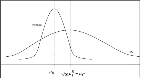
migrants are selected from the upper tail of the income distribution at home and end up in the upper tail of the income distribution abroad (in both cases, the relevant distribution is the origin country’s population one). For example, consider potential migrants from Portugal to the United States (Figure 2). Given that income inequality is lower in Portugal than in the U.S. and assuming thatρ01is sufficiently high, among Portuguese workers it’s the better-off
24The reason is that, with higherID
01, the range ofµ01(µ0) for which the effect is strictly positive (negative) is wider.
25Formulas (14) and (15) are based on the expression for dP in footnote 22 (given that immigration quotas are not binding, then I01
P0 =P). If quotas are not binding (η01 = 1), assuming that σC = 0, then:
dσv= [σ21+σ20−2ρ01σ0σ1]−
1
2[(σ1−ρ
01σ0)dσ1+ (σ0−ρ01σ1)dσ0−σ0σ1dρ01]. Notice that, in formula (14) and (15),k=φ(z)(σ21+σ20−2ρ01σ0σ1)−
1 2(−1
σ2
who have an incentive to migrate while those at the lower tail of the income curve have an incentive to stay. The reason is that the probability of both very high and very low incomes is higher in the U.S. than in Portugal. An increase in income inequality in Portugal will
make individuals at the bottom of the income distribution relatively worse-offat home and
will increase their incentive to leave. Similarly, if σ0
σ1 >1andρ01is sufficiently high (ρ01>
σ1
σ0), thendσ0 >0ordσ1 <0(i.e., an
increase in the relative inequality σ0
σ1) will decrease the emigration rate. Given that income is
more dispersed at home than abroad, this is the case of negative selection of immigrants from country0to country1(Borjas 1987): migrants are selected from the lower tail of the income distribution at home and end up in the lower tail of the income distribution abroad. An example of this situation is migration from Brazil to the U.S., given that income inequality in the latter is lower than in the former (Figure 2). An increase in income inequality in Brazil will lower the emigration rate because those who were not migrating beforehand, the better-off, will have even less incentive to do so afterwards.
Notice that, in a way similar to the impact offirst moments, the effect of second moments will be affected by whether immigration quotas are binding or not.
Finally, a few extensions of this simple theoretical framework deliver interesting predic-tions that I will discuss and investigate in the empirical section.
3
Data
In this paper, I combine an international panel data set on bilateral immigration flows with additional macroeconomic and non-economic data on the origin and destination country of each immigrantflow. Data on immigration comes from the International Migration Statistics (IMS) data set for OECD countries (OECD 1997), which contains information on immigrant
flows by country of origin, based on the OECD’s Continuous Reporting System on Migration
(SOPEMI).26 Population registers and residence and work permits are the main sources of
these statistics. In particular, I use data on yearly immigrant inflows into fourteen OECD countries by country of origin, in the period 1980-1995. Appendix 2, at the end of the paper, presents summary statistics on immigrant inflows by host and source country, averaged over the years 1980-1995 (see also Figure 3).
Appendix 3 shows that the disaggregate (i.e., by country of origin) IMS statistics on
migrant flows don’t add up to 100% of the total flow into each destination country. The
percentage of the total immigrant inflow covered by the disaggregate data ranges between
45% (Belgium) and 84% (United States). Put differently, the data set includes zeroflows in
correspondence of some country pairs (immigrant inflows from Italy to the United States,
for example). Some of these observations correspond to truly zero flows, while others are
likely to correspond to very small flows. If the latter observations are recorded as zeros in
the disaggregate data set, there will be a discrepancy between total flows and the sum of
flows by origin country. In the empirical analysis I will keep zero-flows observations in the data set.27 I will also investigate the robustness of my results using a Tobit model.28
Summary statistics and data sources of each variable used in the empirical model are documented in Appendix 1. Data on macroeconomic variables comes from various sources: the 2001 World Development Indicators (World Bank 2001), the Penn World Tables (versions 5.6 and 6.1), and the World Bank’s Global Development Network Growth Database, Macro Time Series (Easterly and Sewadeh 2002). Geographical and cultural information, such as on great-circle distance, land border, common language, and colonial ties, comes from Glick and Rose’s (2001) data set on gravity-model variables. I also use statistics on the average number of schooling years in the total population (over age 15) from Barro and Lee’s (2000) data set.29 Data on Gini coefficients of destination and origin countries, used to construct the origin country’s relative inequality variable, comes from Deininger and Squire (1996) data set (only high-quality observations were used). Finally, information on origin countries’ share of young population comes from the United Nations.
A separate Appendix to the paper documents the main characteristics of the migration policies of the destination countries in the sample and the timing (after 1980) of changes in their legislations (Mayda and Patel, 2004).30 A data set of destination countries’ migration-policy changes, between 1980 and 1995, was constructed on the basis of the information in this Appendix and used in the empirical analysis.
4
Empirical model
The theoretical framework in Section 2 suggests an empirical specification characterized by the emigration rate as the dependent variable and, among the explanatory variables, the mean wage of the origin country’s population in, respectively, the origin and destination countries. As approximations for the latter two variables, I use the (log) level of per worker
GDP, PPP-adjusted (constant 1996 international dollars) in the two countries.31 Based on
the basic model, I expect pull effects to be positive on average and push effects to be negative on average.
Another determinant of bilateral immigration flows implied by the model of Section 2
is the distance between the two locations, which affects migration costs Ci. The further
27The results don’t change when I drop zero observations (see previous version of this paper). 28See regression (4), Table 4.
29Since this panel only contains data atfive-year intervals (in the period I consider, the years covered are 1980, 1985, 1990, 1995), I linearly extrapolatefigures for the in-between years (by assigning onefifth of the five-year change in the variable to each year).
30The Appendix can be found in my website.
31Per worker GDP is not a direct measure of the mean wage of the origin country’s population at home and abroad. See below for robustness checks related to this point.
away the two countries are, the higher the monetary travel costs for the initial move, as well as for visits back home. Remote destinations may also discourage migration because they require longer travel time and thus higher foregone earnings. Another explanation
as to why distance may negatively affect migration is that it is more costly to acquire
information ex-ante about far-away countries (Greenwood 1997 and Lucas 2000). I introduce additional variables that affect the level of migration costs Ci. A common land border is likely to encourage migrationflows, since land travel is usually less expensive than air travel. Linguistic and cultural similarity are also likely to reduce the magnitude of migration costs, for example by improving the transferability of individual skill from one place to the other. Past colonial relationships should increase emigration rates, to the extent that they translate into similar institutions and stronger political ties between the two countries, thus decreasing the level of migration costsCi.
In a cross-country analysis, such as in this paper, unobserved country-specific effects could result in biased estimates. For example, I may estimate a positive coefficient on the destination country’s per worker GDP. Based on this result, it is not clear whether immi-grants go to countries with higher wages or, alternatively, whether countries with higher wages have other features that attract immigrants. Along the same lines, a negative
coef-ficient on income at home leaves open the question of whether immigrants leave countries
with lower wages or, alternatively, whether countries with lower wages have certain charac-teristics that push immigrants to leave. To (partly) get around this problem, I exploit the panel structure of the data set and I introduce dummy variables for both destination and origin countries. This allows me to control for unobserved country-specific effects which are additive and time-invariant. All specifications in Tables 1, 4, 5, and 6 include destination and origin countries’ fixed effects and have robust standard errors clustered by country pair, to address heteroscedasticity and allow for correlation over time of country-pair observations.32 Notice that destination country fixed effects allow me to control for features of destination countries’ immigration policy which don’t change over time and are common across origin countries. In order to capture the effect of changes in destination countries’ migration poli-cies, I introduce two interaction terms of an indicator variable of such changes with pull and push factors, respectively. According to the theory, if the migration policy of a destination country becomes less restrictive, the effect of pull (push) factors should turn more positive (negative).
Finally, I introduce the share of the origin country’s population who is young (between 15
and 29 years old) as a demographic determinant of migration flows. Consider an extension
of the basic model in Section 2 to a multi-period setting. In this set-up, the individual cares not only about current wage differentials net of moving costs, but about future ones too. As Clark, Hatton, and Williamson (2002) point out, this implies that a potential migrant from country0will have a bigger incentive to migrate the younger he is, as the present discounted
32Most specifications in the tables include separate dummy variables for destination and origin countries, while the remaining regressions control for country-pairfixed effects.
value of net benefits will be higher the more extended the length of the remaining work life time (for positiveIi in each year). We would then expect the share of young population in the origin country to increase the emigration rate out of that country.
The basic empirical specification thus looks as follows:
f lowijt
Pit =β+β0pwgdpit−1+β1pwgdpjt−1+β2distij +β3borderij +β4comlangij+β5colonyij+
+β6youngpopit−1+β7pwgdpit−1·immigpoljt +β8pwgdpjt−1·immigpoljt+εijt (16) whereiis the origin country,jthe destination country andttime. f lowijt
Pit is the emigration
rate fromi to j at time t (f lowijt is the inflow into country j from countryi at time t, Pit
is the population of the origin country at time t). pwgdp is the (log) per worker GDP,
PPP-adjusted (constant 1996 international dollars) and distmeasures the (log) great-circle
distance between the two countries. The variable border equals one if the two countries in
the pair share a land border. comlang and colony are two dummy variables equal to one,
respectively, if a common language is spoken in both locations, and for pairs of countries which were, at some point in the past, in a colonial relationship. Finally, youngpop is the share of the population in the origin country aged 15-29 years old and the variableimmigpol
equals one (minus one) if in that year the destination country’s immigration policy became less (more) restrictive (zero otherwise). According to the theory, I expect that β0 < 0,
β1 >0, β2 <0,β3 >0,β4 >0, β5 >0, β6 >0, β7 <0, and β8 >0.
I will next discuss a few econometric issues that affect the interpretation of pull and push
coefficients. First, assuming that per worker GDP proxies for the mean income opportunity
of the origin country’s population in each location (see below for a discussion of this point), an empirical complication is the possibility of reverse causality and, more in general, of endogeneity in the time-series dimension of the analysis. The theoretical model in Section 2 predicts that,ceteris paribus, higher (lower) income opportunities in the destination (origin) country increase emigration rates. However, a positive β1 (negative β0) may just reflect
causation in the opposite direction, i.e. the impact of immigrant flows on wages (or levels of per worker GDP) in the host and source country. After all, this channel is the focus of analysis in most labour-economics papers (see Friedberg and Hunt 1995 for a survey of this literature). More broadly, other time-variant third factors may drive contemporaneous
wages and immigrant flows.
As for reverse causality, notice that it is likely to bias the estimates toward zero. The
reason is that immigrant inflows are likely to decrease wages in the destination country
and outflows are likely to increase wages in the origin country. While the opposite signs are a theoretical possibility (for example, in the economic-geography literature, because of economies of scale), the empirical evidence in the labor-economics literature is that immigrant
inflows have a negative impact on the destination country’s wages (Borjas 2003) and that immigrant outflows have a positive impact on the origin country’s wages (Mishra 2003).
I address reverse-causality and endogeneity issues in two ways. First of all, in the basic specification, I relate current emigration rates to lagged values of (log) per worker GDP, at home and abroad. Indeed, while it is hard to claim that wages at home and abroad are strictly exogenous, it is plausible to assume that they are predetermined, in the sense that immigrant inflows - and third factors in the error term - only affect contemporaneous and future wages.33
I next use instrumental-variables estimation with countries’ terms of trade as an instru-ment for PPP-adjusted income levels in the destination and origin country. Papers in the literature where shocks to terms of trade are used as instruments for growth rates of in-come are, for example, Pritchett and Summers (1996) and Easterly, Kremer, Pritchett and Summers (1993).
To capture the effect of income opportunities for a potential migrant at home and abroad, I use data on per worker GDP (PPP-adjusted) in the origin and destination country. How-ever, per worker GDP is not a direct measure of such income opportunities, since it depends on rates of return to both capital and labor and on per worker endowments of each factor. In other words, a higher per worker GDP in the destination country does not necessarily mean better income opportunities on average for a worker from the origin country, since it could be due to a higher capital-labor ratio or to a more skilled labor force in the destination country’s population. In order to focus on rates of return to labor, I will run a robustness check and control for the mean skill level and per worker endowment of capital in each country.34
The last set of predictions of the model in Section 2 (formulas (14) and (15)) is related to the second moment of the income distributions in the origin and destination country.
According to the theory, given low values of σ0
σ1, if
σ0
σ1 increases, the emigration rate will
increase, while given high values of σ0
σ1, if
σ0
σ1 increases, the emigration rate will decrease. In
order to test this prediction, I introduce in the model the origin country’s relative inequality (σ0
σ1) in linear and quadratic form. I expect the coefficient on the linear term to be positive
and on the quadratic term to be negative (Clark, Hatton, and Williamson 2002).
A few extensions of the simple theoretical framework in Section 2 deliver interesting pre-dictions that I investigate empirically. First, it is possible to incorporate poverty constraints into the model, due tofixed costs of migration and credit market imperfections in the origin country. As Young (2003) shows, these assumptions imply that the effect on emigration rates of income opportunities at home is non-monotonic, positive at very low levels of income and
33Strict exogeneity of an explanatory variable implies E[X
itεis] = 0, for ∀s, t, while predeterminacy
impliesE[Xitεis] = 0, for∀s > t. In one of the following specifications, I also control for lagged values of
the emigration rate, since if the emigration rate is autocorrelated, predeterminacy of the regressors does not guarantee consistency of the estimates.
34International differences in rates of return to capital also matter but, as a first approximation, I will assume that capital is internationally mobile.
negative for higher levels. Accordingly, I extend the empirical model previously specified by introducing both a linear and a quadratic term in per worker GDP of the origin country.
Second, the theoretical model can be modified by considering in (8) the expected wage, both in the origin and destination country, given uncertainty of finding a job in each place.
The probability of finding a job can be approximated by one minus the unemployment rate,
which I introduce as a regressor in the empirical specification.
Finally, an important extension is to consider the possibility for workers to choose among multiple destination countries. In this framework, potential migrants compare mean income opportunities in their origin country to those in the destination country considered and in any other host country. For each pair of source and host economies, I construct and control for amultilateral pull term which is an average of per worker GDPs of all the other destination countries in the sample (each weighted by the inverse of distance from the origin country).
To conclude, I investigate the role of past migrationflows to the destination country from the same origin country. The latter ones affect the current emigration rate through both the supply and the demand channel. On the supply side, lagged emigration rates or, alternatively,
the size of the immigrant stock from the same source country, proxy for network effects,
which are likely to reduce the cost Ci of migration. On the demand side, past migration
flows influence the emigration rate in two ways: through family-reunification immigration policies and through political-economy factors (see, for example, Goldin (1994) and Ortega (2004), where the votes of naturalized immigrants affect immigration policy outcomes). The introduction of the lagged emigration rate among the explanatory variables makes the model a dynamic one. I use Arellano and Bond’s GMM estimator to deal with the incidental parameter problem that arises withfixed-effects estimation of such a dynamic equation.35
5
Empirical results
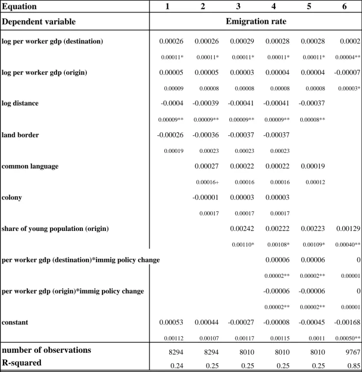
Table 1, at the end of the paper, presents the results from estimation of equation (16) exploiting both the cross-country and time-series variation in the data.
The estimates of Table 1 show a systematic pattern, broadly consistent with the theoret-ical predictions of the basic international-migration model. The emigration rate is positively related to the destination country’s (log) per worker GDP, as predicted in Section 2. Accord-ing to the estimate in regression (1), a ten percent increase in the level of per worker GDP in the destination country increases emigration by 2.6 emigrants per 100,000 individuals of the origin country’s population. In other words, a 10% increase in the host country’s per worker GDP implies a 19% increase in the emigration rate (as the mean of the dependent variable is,
35In a dynamic equation, thefixed effects (or within) estimator of the coefficient of the lagged dependent variable is consistent as T → ∞, for given N, but it is not consistent for given T, asN → ∞ (incidental parameter problem). The intuition behind this result is that, in the latter case, the number of parameters to be estimated tends to infinity, while the information used to estimate each parameter does not increase.
in regression (1), 14 emigrants per 100,000 individuals). The impact on the emigration rate of a change in the income opportunities at home is not consistent with the predictions of the basic model. Push effects are estimated to be insignificantly different from zero. As pointed out above, one reading of this result is that it is driven by the effect of poverty constraints in the origin country. I will investigate this possibility in Table 5.
In Table 1 I also explore the role played by geographical (log distance andland border),
cultural (common language and colony), and demographic (share of young population
(origin)) determinants, respectively. Controlling for destination and origin countries’ fixed effects, the picture that emerges from my results is one in which geography and
demograph-ics are the most important non-economic determinants of migrationflows. According to the
estimate in column (1), doubling the great-circle distance between the source and host coun-try decreases the number of emigrants by 40 per 100,000 individuals in the origin councoun-try (significant at the 1% level). On the other hand, a common land border does not appear to play a significant role. The impact of a common language, though of the right sign, is not always statistically significant and, surprisingly, past colonial relationships do not appear to significantly affect migration rates. Finally, the share of the origin country’s population who is young has a positive and significant impact on emigration rates. A ten percentage point increase in the origin country’s 15-29 years old population raises the emigration rate by 24 emigrants per 100,000 individuals (regression (3)).
Next, I investigate the interaction between changes in destination countries’ migration policies and, respectively, pull and push factors (column (4), Table 1). Consistent with the theoretical predictions, positive pull factors are bigger (smaller) than average for a desti-nation country whose migration policy becomes less (more) restrictive. Push factors turn negative and significant once migration restrictions are relaxed.36
Finally, in regression (6) I only exploit the variation over time within country pairs, by in-troducing dummy variables for each combination of origin and destination countries.37 These country-pairs fixed effects allow me to control for time-invariant features of the destination country’s immigration policy which are specific for each origin country.
The specifications in Tables 2 and 3 are the most closely related to trade gravity-model regressions (which are usually estimated in a cross section). In Table 2 I focus on a subset of determinants and estimate their coefficients by exploiting only the cross-country variation in the data. I divide the period between 1981 and 1995 into three segments and I focus on each at a time. I relate average emigration rates in each subperiod to the average income
opportunities at home and abroad in the previous five-year interval (plus time-invariant
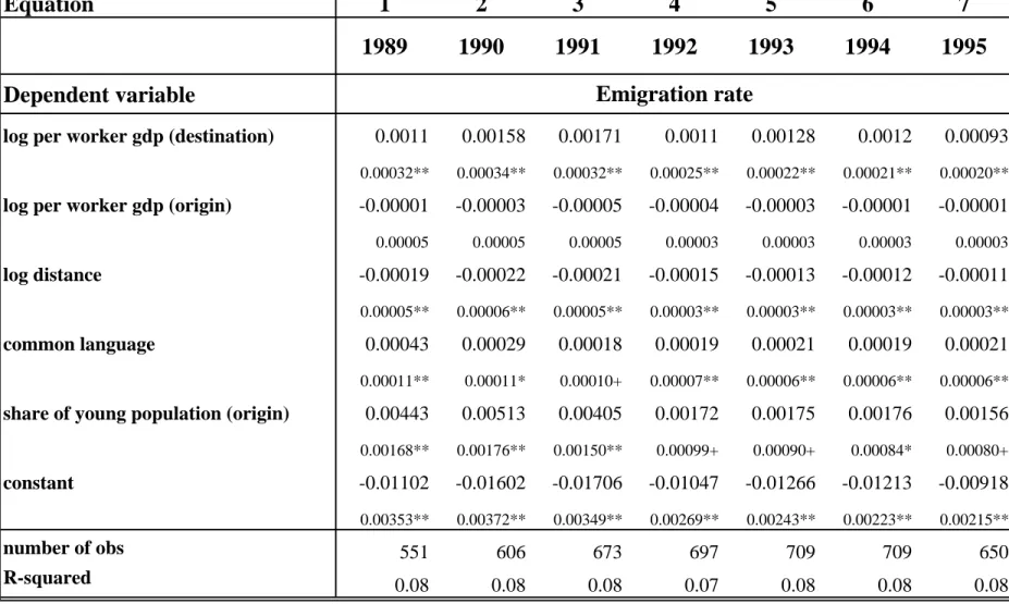
variables). In Table 3 I perform a similar exercise by estimating the model year by year. Due to the low number of observations in each regression, in Table 2 and Table 3 I don’t
36Interestingly, the coefficients of the two interaction variables are equal in absolute value.
37Regression (6) does not include the regressorslog distance, land border, common language and colony since they are constant within country pairs and, therefore, they would be perfectly collinear with the dummy variables.
control for country-specificfixed effects, which explains the difference in the magnitude of the effects relative to the regressions in Table 1. The coefficients are still qualitatively consistent with the panel-data results, though less precisely estimated.
In Table 4 I run a few robustness checks of the panel-data results. In thefirst regression, I use (within-country variation in) the terms of trade to instrument for (within-country variation in) the level of per worker GDP of both destination and origin countries. Terms of trade are correlated with the average real income of a country since they affect countries’ purchasing power vis a vis goods produced by the rest of the world. In the first stage, the impact of the terms of trade on per worker GDP is positive and significant at the 1% level, for both destination and origin countries. In addition, if the assumption of small open economies holds, terms of trade are unlikely to affect emigration rates directly or to be correlated with other country-level characteristics that have an impact on migration patterns (exclusion restriction). Regression (1) shows that pull and push coefficients are robust to endogeneity issues as the instrumental variable estimates are consistent with my earlier results.
In columns (2) and (3), I ask whether per worker GDP in the two locations is a good
measure of the mean income opportunities for migrant workers at home and abroad. I first
control for the average schooling level in both countries in specification (2). Pull effects are still estimated to be positive and significant (at the 1% level). In line with the theoretical predictions, the average skill level in the population of the destination (origin) country has a negative (positive) impact on the emigration rate. In column (3) I control for per worker endowments of both skill and capital and againfind that my prior findings are robust.
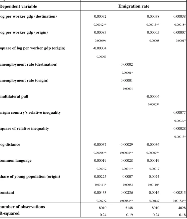
In Table 5 I examine the predictions based on the extensions of the theoretical framework of Section 2. I find only weak evidence of poverty constraints in regression (1) and confirm, in the following specification, my results on push and pull factors in terms of unemployment
rates. Third-country effects shape bilateral migration flows as expected, given that the
coefficient on the multilateral pull term is negative and significant.38 Finally, the size of
emigration rates is affected by the second moments of the income distributions in the two
location in the way predicted by Borjas (1987) selection model.
To conclude, I analyze network effects by introducing the lagged emigration rate(s) among the explanatory variables (Table 6). Emigration rates clearly show a lot of inertia. How-ever, it’s unclear whether supply or demand factors explain the autocorrelation in bilateral migration flows.39
38The multilateral pull term places migrants’ decision to move in a multi-country framework. It is inspired by the multilateral trade resistance term in Anderson and van Wincoop (2003) (even though mine is an atheoretical measure).
39Fixed-effects estimation of a dynamic model with a short panel (small T) produces biased estimates. This might explain the estimates in thefirst two columns of push and pull factors (which are different from previous ones). Once I use Arellano and Bond’s estimator, the coefficients become consistent with what I previously found.
6
Conclusions
In this paper, I investigate economic and non-economic determinants of international migra-tionflows. This analysis both delivers estimates consistent with the predictions of a standard international-migration model and generates empirical puzzles.
In particular, I find that pull factors, that is improvements in the income opportunities in the destination country, significantly increase the size of emigration rates. This result, which appears to be very robust to changes in the specification of the empirical model, is surprising, given very restrictive immigration policies of the destination countries included in the sample. The sign of the impact of push factors - that is, declining levels of per worker GDP in the origin country - is seldom consistent with the theoretical predictions of the model and, when it is, the size of the effect is smaller than for pull factors and is almost always insignificant. Among the variables affecting the costs of migration, distance appears to be one of the most important ones. Its effect is negative, significant and quite steady across specifications.
The investigation of the determinants of international migration leads to other interesting research questions. This analysis provides a framework to address policy-related issues, as has been done in the trade gravity-model literature. The analysis of the impact of labour movements on source and host economies - on their standards of living, for example - faces
the inherent problems of endogeneity of migration flows and reverse causality. Since this
work helps isolate the exogenous determinants of immigrantflows, it is possible to use it to construct afirst stage for this type of analyses (as in Frankel and Romer 1999, for example). By taking advantage of both the time-series and cross-country variation in an annual panel data set, this paper makes progress in explaining the economic and non-economic determinants of international migration flows.
References
Adams, R. H. J. (1993). The economic and demographic determinants of international
migration in rural Egypt. Journal of Development Studies, 30(1):146—167.
Barro, R. and Lee, J. (2000). International data on educational attainment. Data Set.
Benhabib, J. (1996). On the political economy of immigration. European Economic Review,
40:1737—1743.
Borjas, G. and Bratsberg, B. (1996). Who leaves? The outmigration of the foreign-born. Review of Economics and Statistics, 78(1):165—176.
Borjas, G. J. (1987). Self selection and the earnings of immigrants. American Economic
Borjas, G. J. (1994). The economics of immigration. Journal of Economic Literature, pages 1667—1717.
Borjas, G. J. (1995). The economic benefits from immigration. Journal of Economic
Per-spectives, 9(2):3—22.
Borjas, G. J. (1999a). The economic analysis of immigration. In Ashenfelter, O. and Card,
D., editors, Handbook of Labor Economics, chapter 28, pages 1697—1760. North-Holland
Elsevier Science, The Netherlands.
Borjas, G. J. (1999b). Heaven’s Door: Immigration Policy and the American Economy.
Princeton University Press, Princeton, N.J.
Borjas, G. J. (2003). The labor demand curve is downward sloping: Reexamining the impact
of immigration on the labor market.The Quarterly Journal of Economics, 40:1335—1374.
Harvard University.
Chiswick, B. R. and Hatton, T. J. (2002). International migration and the integration of
labour markets. In Globalization in Historical Perspective. The University of Chicago
Press, Chicago, IL. Forthcoming.
Clark, X., Hatton, T. J., and Williamson, J. G. (2002). Where do U.S. immigrants come from, and why? National Bureau of Economic Research Working Paper No. 8998. Coppel, J., Dumont, J.-C., and Visco, I. (2001). Trends in immigration and economic
consequences. OECD Economics Department Working Papers No. 284.
Davies, J. B. and Wooton, I. (1992). Income inequality and international migration. The
Economic Journal, 102(413):789—802.
Davis, D. R. and Weinstein, D. E. (2002). Technological superiority and the losses from migration. National Bureau of Economic Research Working Paper No. 8971.
Easterly, W., Kremer, M., Pritchett, L., and Summers, L. H. (1993). Good policy or good
luck? Country growth performance and temporary shocks. Journal of Monetary
Eco-nomics, 32:459—483.
Easterly, W. and Sewadeh, M. (2002). Global development network growth database, Macro time series. World Bank. Data Set.
Facchini, G. and Willmann, G. (2005). The political economy of international factor mobility. forthcoming Journal of International Economics.
Faini, R. (2002). Discussion of "International migration and the integration of labor markets" by B. Chiswick and T. Hatton. InGlobalization in Historical Perspective.The University of Chicago Press, Chicago, IL. Forthcoming.
Faini, R. and Venturini, A. (1994). Trade, aid and migrations. Some basic policy issues. European Economic Review, 37:435—442.
Frankel, J. A. and Romer, D. (1999). Does trade cause growth? The American Economic
Review, 89:379—399.
Freeman, G. (1992). Migration policy and politics in the receiving states. International
Migration Review, 26(4):1144—1167.
Freeman, G. (1995). Modes of immigration politics in liberal democratic states.International Migration Review, 29(4):881—902.
Friedberg, R. and Hunt, J. (1995). The impact of immigrants on host country wages,
em-ployment, and growth. Journal of Economic Perspectives, 9(2):23—44.
Goldin, C. (1994). The political economy of immigration restriction in the United States,
1890 to 1921. In Goldin, C. and Libecap, G., editors, The Regulated Economy: A
Historical Approach to Political Economy, pages 223—257. University of Chicago Press, Chicago, IL.
Greenwood, M. J. (1997). Internal migration in developed countries. In Rosenzweig, M.
and Stark, O., editors,Handbook of Population and Family Economics, Vol. 1B.
North-Holland, Amsterdam.
Hatton, T. J. and Williamson, J. G. (2003a). Demographic and economic pressure on
emi-gration out of Africa. Scandinavian Journal of Economics, 105:465—482.
Hatton, T. J. and Williamson, J. G. (2003b). What fundamentals drive world migration? revised version of National Bureau of Economic Research Working Paper No. 9159, forthcoming in G. Borjas and J. Crisp (eds), Poverty, international migration and asy-lum, Palgrave-Macmillan.
Helliwell, J. F. (1997). National borders, trade and migration. National Bureau of Economic Research Working Paper No. 6027.
Helliwell, J. F. (1998). How Much Do National Borders Matter?, chapter 5, pages 79—91.
Brookings Institution Press.
Heston, A., Nuxoll, D. A., Summers, R., and Aten, B. (1995). Penn World Table version 5.6a. Data Set.
Heston, A., Summers, R., and Aten, B. (2002). Penn World Table version 6.1. Center for International Comparisons at the University of Pennsylvania (CICUP). Data Set. Hoddinott, J. (1994). A model of migration and remittances applied to Western Kenya.
Oxford Economic Papers, 46:459—476.
ILO (1998). International labour migration database. International Labor Organization. Jenks, R. (1992).Immigration and Nationality Policies of Leading Migration Nations.Center
for Immigration Studies, Washington, DC.
Joppke, L. (1998). Why liberal states accept unwanted immigration. World Politics, 50:266— 293.
Karemera, D., Oguledo, V. I., and Davis, B. (2000). A gravity model analysis of international
migration to North America. Applied Economics, 32(13):1745—1755.
Lucas, R. E. (2000). The effects of proximity and transportation on developing country
population migrations. Boston University.
Mayda, A. M. (2003). Who is against immigration? A cross-country investigation of indi-vidual attitudes toward immigrants. Harvard University, dissertation chapter.
Mayda, A. M. and Patel, K. (2004). OECD countries migration policies changes. Appendix to International Migration: A Panel Data Analysis of Economic and Non-Economic Determinants, by Anna Maria Mayda. http://www.georgetown.edu/faculty/amm223/. Money, J. (1997). No vacancy: The political geography of immigration control in advanced
industrial countries. International Organization, 51:685—720.
OECD (1997). International migration statistics for OECD countries. Data set.
OECD (2001). The employment of foreigners: Outlook and issues in OECD countries. In OECD Employment Outlook, chapter 5. OECD, Paris.
Pritchett, L. and Summers, L. H. (1996). Wealthier is healthier. The Journal of Human
Resources, 31(4):841—868.
Ravenstein, E. (1885). The laws of migration. Proceedings of the Royal Statistical Society, XLVII(2):167—235.
Rodrik, D. (1995). Political economy of trade policy. In Grossman, G. and Rogoff, K.,
edi-tors, Handbook of International Economics, Vol.3, chapter 28, pages 1457—1494.
SOPEMI (1997). Trends in International Migration. Annual Report 1996. OECD, Paris.
SOPEMI (1999). Trends in International Migration. OECD, Paris.
SOPEMI (2000). Trends in International Migration. OECD, Paris.
Trefler, D. (1997). Immigrants and natives in general equilibrium trade models. National
Bureau of Economic Research Working Paper No. 6209.
Yang, D. (2003). Financing constraints, economic shocks, and international labor migra-tion: Understanding the departure and return of philippine overseas workers. Harvard University, dissertation chapter.
Yang, P. Q. (1995). Post-1965 Immigration to the United States. Praeger, Westport,
Equation 1 2 3 4 5 6 Dependent variable
log per worker gdp (destination) 0.00026 0.00026 0.00029 0.00028 0.00028 0.0002
0.00011* 0.00011* 0.00011* 0.00011* 0.00011* 0.00004**
log per worker gdp (origin) 0.00005 0.00005 0.00003 0.00004 0.00004 -0.00007
0.00009 0.00008 0.00008 0.00008 0.00008 0.00003* log distance -0.0004 -0.00039 -0.00041 -0.00041 -0.00037 0.00009** 0.00009** 0.00009** 0.00009** 0.00008** land border -0.00026 -0.00036 -0.00037 -0.00037 0.00019 0.00023 0.00023 0.00023 common language 0.00027 0.00022 0.00022 0.00019 0.00016+ 0.00016 0.00016 0.00012 colony -0.00001 0.00003 0.00003 0.00017 0.00017 0.00017
share of young population (origin) 0.00242 0.00222 0.00223 0.00129
0.00110* 0.00108* 0.00109* 0.00040**
per worker gdp (destination)*immig policy change 0.00006 0.00006 0
0.00002** 0.00002** 0.00001
per worker gdp (origin)*immig policy change -0.00006 -0.00006 0
0.00002** 0.00002** 0.00001
constant 0.00053 0.00044 -0.00027 -0.00008 -0.00045 -0.00168
0.00112 0.00107 0.00117 0.00115 0.0011 0.00050**
number of observations 8294 8294 8010 8010 8010 9767
R-squared 0.24 0.25 0.25 0.25 0.25 0.85
per worker gdp is the level of per worker GDP, PPP-adjusted (constant 1996 international dollars), lagged by one year.
distance is the great-circle distance. Land border equals one if the destination and origin countries share a land border.
common language equals one if a common language is spoken in both destination and origin countries.
colony is a dummy variable for pairs of countries ever in a colonial relationship.
share of young population (origin) is the share of the population in the origin country aged 15-29.
Emigration rate
Table 1. Panel data regressions
OLS estimates. Destination and origin countries' dummy variables are included in each specification, except the last one (in regression 6, country-pairs dummy variables are included). Standard errors, clustered by country pairs, are presented under each estimated coefficient. + significant at 10%; * significant at 5%; ** significant at 1%
immigration policy change equals one if in that year the destination country's immigration policy became less restrictive, minus one if it became more restrictive, zero if there was no change in immigration policy.
2
R 2
Equation
1
2
3
1981-1985
1986-1990
1991-1995
Dependent variable
log per worker gdp (destination)
0.00028 0.00068 0.000880.00015+ 0.00022** 0.00020**
log per worker gdp (origin)
-0.00002 -0.00004 -0.000040.00003 0.00004 0.00003
log distance
-0.00007 -0.0001 -0.0001 0.00003* 0.00004* 0.00003**common language
0.00037 0.0004 0.00025 0.00007** 0.00008** 0.00007**constant
-0.00208 -0.00592 -0.00809 0.00166 0.00240* 0.00222**number of obs
571 628 709R-squared
0.06 0.06 0.06OLS estimates. The standard errors are presented under each estimated coefficient. + significant at 10%; * significant at 5%; ** significant at 1%
distance is the great-circle distance.
common language is a dummy variable equal to one if a common language is spoken in both destination and origin countries. See Appendix 1 for data sources.
Emigration rate
Table 2. Cross-country regressions
per worker gdp is the level of per worker GDP, PPP-adjusted (constant 1996 international dollars), averaged over the five years preceding the relevant period (1976-1980 for the regression in column (1), for example).
2
R 2