Enhancing Simulation Models for Open Pit Copper Mining. Using Visual Basic for Applications

(1)

* Chuo Gakuin University, Faculty of Commerce

■ 2012 JSPS Asian Core Program, Nagoya University and VNU University of Economics and Business

Enhancing Simulation Models for Open Pit Copper Mining

Using Visual Basic for Applications

Chuo Gakuin University Yifei TAN*

ABSTRACT:

In open pit mining operations, the diesel consumption of haul trucks represents roughly 50% of the total operating costs. To reduce operating costs, the trucks must be allocated and dispatched efficiently. In this study, a simulation model of open pit copper mining has been enhanced using Visual Basic for Applications (VBA) programming, which can be used to test and create a truck dispatching control table to satisfy a mining plan. By combining the simulation technique with the utilization of Excel and VBA programming, the enhanced simulation model could aid managers in mining operations decisions.

KEYWORDS: Open Pit Mining, Simulation, Truck Dispatching, VBA Programming

1 INTRODUCTION

In open pit mining operations, haul trucks‟ diesel consumption accounts for the largest portion of operating costs. As other studies have demonstrated, transportation costs represent roughly 50% of the operating costs in an open pit mine (Alarie and Gamache, 2002; Ercelebi and Bascetin, 2009). In this context, the trucks must be efficiently allocated and dispatched to reduce operating cost.

An open pit copper mine usually comprises two major components, the open pit mining operation and the copper ore enrichment plant. At present, the mining industry is a strong foundation of Mongolian economic growth. In 2007, according to the Mongolian Statistical Yearbook, Mongolia‟s overall GDP grew by 8.4% and that of the mining sector grew by 2.7%. High international gold and copper prices have driven exploitation of new mines and increased this sector‟s

production. The mining industry is required to flexibly respond to trends in world market demands, and companies must improve their mining operations and transportation of mined products.

This study applies computer simulation techniques to support open pit mining operations management. After a brief description of the simulation‟s application in the mining industry, we present a case study utilizing simulation techniques to solve an open pit mine truck dispatching problem. Simulation models are constructed and applied by utilizing GPS (Global Positioning System) tracking data to evaluate the current state of operations for an open pit mining company. Then, the simulation model is enhanced with Excel and Visual Basic for

Applications (VBA) programming, which enable

testing and creation of a truck dispatching control table to satisfy a mining plan.

(2)

2 OPERATIONS AND SIMULATION IN THE MINING INDUSTRY

There are two general approaches to mining: open pit (i.e., surface) mining and underground mining. The mining industry faces problems that are growing in both size and complexity. Production is dependent on the geological position of the ore body and the technology for extraction, which involves the use of expensive capital equipment. Simulations can support management decisions for daily production and capital expenditures, providing a visual and dynamic demonstration of system behavior optimization through various strategies (Chinbat and Takakuwa, 2009).

In the open pit mining operation, a materials handling system consists of subsystems for loading, hauling, and dumping. Truck haulage is the most common means of moving ore/waste in open pit mining operations, but is also the most expensive unit of operation in a truck-shovel mining system (Kolojna et al., 1993). Bauer and Calder (1973) noted that the complexity of modern open pit load-haul-dump systems requires realistic working models. Nenonen et al. (1981) studied an interactive computer model of truck-shovel operations in an open pit copper mine. Qing-Xia (1982) studied a computer simulation program of drill rigs and shovel operations in open pit mines.

As Subtil et al. (2011) states, “In the specific context of the mining industry, the truck dispatch problem in open pit mining is dynamic and consists in answering the following question: „Where should this truck go when it leaves this place?‟‟‟ Two goals were targeted to solve the dispatching problems: increase productivity and reduce operating costs (Alarie and Gamache, 2002). Burt et al. (2005) conducted a critical analysis of the various models used for surface mining operations, identifying important constraints and suitable objectives for an equipment selection model.

They used a new mixed integer linear programming (LP) model that incorporates a linear approximation of the cost function. Fioroni et al. (2008) proposed concurrent simulation and optimization models to achieve a feasible, reliable, and accurate solution to the analysis and generate a short-term planning schedule. Ercelebi and Bascetin (2009) studied truck-shovel operation models and optimization approaches for allocating and dispatching truck under various operating conditions. They used the closed queuing network theory for truck allocation and LP to dispatch trucks to shovels. Boland et al. (2009) proposed LP-based disaggregation approaches to solve a production scheduling problem in open pit mining. Subtil et al. (2011) proposed a multistage approach for dynamic truck dispatching in real open pit mine environments, implementing it with a commercial software package.

3 OPEN PIT MINING OPERATION

3.1 System Description of a Mongolian Open Pit Mining Company

Company A is one of the largest ore mining and processing companies in Asia. Similar to most mining plants, company A‟s production process comprises two major components, an open pit mine and a copper ore enrichment plant. The mine and factory are located in Mongolia and have been in continuous operation since 1978. Both the open pit and enrichment plant operate and produce 24 hours a day throughout the year. At present, company A processes 25 million tons of ore per year and produces over 530 thousand tons of copper concentrate and roughly three thousand tons of molybdenum concentrate annually. The following case study is part of a wider joint research project with company A, with the goal of improving mining and transportation operations efficiency in an open pit mine and ore enrichment plant.

(3)

Mining Plan Transportation Control System with GPS Technology Geological Plan and Strategy Financial Data Excavation Standard

Open Pit Mining Operation

(Drilling → Explosion → Truck Loading → Transportation → Ore Feeding and Dispose of Waste)

Enrichment Plant Operation

(Crasher → Ball Mill → Flotation → Thickener → Concentrate → Filter → Drying→ Packing and Storage)

Production Plan of the Enrichment Plant

F ee d b ac k F ee d b ac k Feedback S co p e o f T h is S tu d y

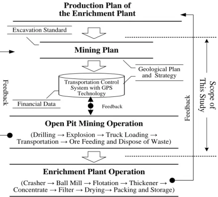
Figure 1: Simplified process map for open pit mining operation in Company “A”

During years of mining, the contents of copper and molybdenum have decreased. Further, in this open pit mine, the contents of copper and molybdenum vary according to the mining location‟s altitude. Specifically, the copper content is lower at low-altitude mining points, where there has been deep digging. However, ore with a copper content below 0.25% cannot be processed under the enrichment plant‟s current technical conditions. Therefore, from the operational management perspective, that is, to preserve the product quality and maintain stable throughput, the copper content of the ore fed to the enrichment plant must remain within required parameters roughly. Therefore, before feeding the ore into the enrichment process, the ores with initially high and low contents of copper must be mixed.

A few years ago, company A implemented a control system for mining transportation with GPS technology. This transportation control system helps company A to technically and economically control the loading and transportation processes.

3.2 Mining Planning

The mining planning stage is crucial in any type of mining because it seeks costs reduction and maximized production plans and focuses on quality and operation requirements, asset utilization, such as trucks, and tractors, and restraints, such as those faced during shoveling (Fioroni et al., 2008). Figure 1 presents a simplified process map for company A‟s open pit mine operation. In company A, when creating a mining plan in accordance with a production plan, that plan must include ores containing both low and high copper content. In company A, the geologist group develops the mining site plan. The open pit mining plan is based on the annual plan, which specifies the volume to excavate from the current altitude of the open pit and evenly distributes the rest to the different altitudes of the mine. The plan also considers the following factors: ore volume, concentrate and oxide levels, and primary ore percentage; geological plan and strategy; ore processing standards; and techn ology of the

(4)

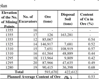
Table 1: An example of a week‟s completed mining plan Elevation of the No. of Mining Points No. of Excavators Ore (tons) Disposal Soil (tons) Content of Cu in Ore (%) 1355 16 - - -1355 17 126 163,281 -1355 12 85,067 - 0.54 1325 14 146,917 7,681 0.52 1310 15 7,651 108,919 0.57 1310 16 61,564 48,889 0.44 1295 18 113,964 9,809 0.42 1295 20 87,966 47,635 0.49 1280 19 90,415 36,398 0.68 593,670 422,612 -0.53 Total

Planned Average Content of Ore_（％）

enrichment plant and excavation standard. Therefore, open pit mine planning relates to the output amount of the production plan for the enrichment factory. It is difficult to determine the best mining positions by considering the required percentage of copper and molybdenum contents, required to satisfy the operations planning of a successful refinery. Table 1 shows an example of a completed mining plan for a given week.

3.3 Transportation and Truck Dispatching

As stated, material (ore and waste soil) transportation in an open pit mine consumes roughly 50% of total operating costs. In this context, efficient truck allocation and dispatching represents a considerable saving of resources. However, the problem of dispatching trucks to excavators is more difficult than it appears.

Table 2 summarizes company A‟s transportation resources. It owns 24 dump trucks, all of which can transport ore or soil from mining points to the enrichment plant or disposal hills, respectively, per the operation center‟s instructions. At the 13 soil disposal locations (hills) around the open pit mining location, the soil is spread over the ground using a bulldozer to recover the environment. The enrichment plant has two ore feeding entrances. When the ore reaches the enrichment plant, it is fed into an ore feeding entrance (bunker A or B) depending upon the size (the diameter) of the ore, and the plant performs the concentrating processes. Table 2 briefly presents the parameters of

Table 2: Company A‟s transportation resources

Number of Units Held 5 units

Number of Operation Shifts 2 shifts

Number of Operation Shifts 3 shifts

Average Productivity per Hour 331.4 m3

/h *

Operation Shifts 3 shifts

Operators 30

Capacity 130 tons

Amount per Transportation TRIA(90,130,147) tons **

Average Distance in a One-way Transportation 3.26 km *

Average Velocity when Loading 24 km/h *

Average Velocity when Unloading 40 km/h *

Operation Shifts 3 shifts

Operators 80

Shift No.1 Shift No.2 Shift No.2 Shifts

Note: * Measures actually vary.

** TRIA indicates a triangular distribution. 8:00-16_：00 16：00-24：00 24：00-8：00 Drillers Bulldozers Excavators Dump Trucks

(5)

certain measures as averaged values.

Although the GPS technology‟s transportation control information system primarily functions to control fuel consumption, weight capacity, and speed of the dump trucks, dispatching a truck to an excavator has not yet been automated due to the complexity involved in dispatching trucks. As described above, to maintain continuous production in the enrichment plant, the content of ore fed to the plant must be kept approximately constant to the required average, a challenging goal. As Table 1 shows, different mining points and locations have different copper content. When calculating the dispatching of a truck to an excavator, dispatchers must determine the truck‟s optimal destination to satisfy the production requirements and its transportation amount. Simultaneously, the dispatchers must consider the progress of transportation at each mining point, because to satisfy the entire mining plan‟s specifications, both the transportation of ore and waste soil must be completed on schedule. Currently, the transport control staff dispatches trucks manually using wireless walkie-talkies and information from the GPS transportation control information system, which is displayed on their computer monitor in real time.

In this study, to facilitate fleet management in open pit mining, we attempt to embed the logic of truck dispatching and automate the dispatching systems. Thus, after the mining plan is complete, when we run the model, the program automatically generates the truck dispatch control table.

4 DEVELOPMENT AND ANALYSIS OF THE

SIMULATION MODEL

4.1 Parameters and Construction of the Simulation Model

Simulations can provide a visual and dynamic system operation description to help mining project managers understand the system‟s behavior and optimize it through various strategies (Chinbat and Takakuwa, 2009). We apply the computer simulation technique to support operations management in company A. The simulation model is programmed in Arena (Kelton et al., 2010) and overlaid on a scaled mine layout. As described, company A has implemented a mining transportation control system with GPS technology. The GPS tracking data and other associated information update the simulation at 1-minute intervals; the important parameters, such as the truck location, its fuel level, and load weight are shown on the open pit map.

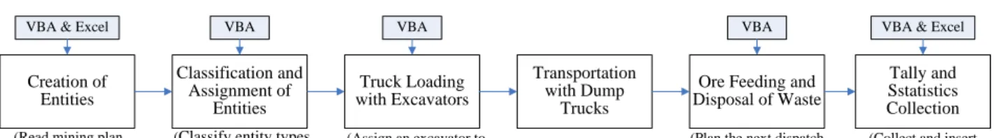
Figure 2 illustrates the overall structure and flow of the simulation model. To understand the current (As-Is) state of mining operations, we initially construct the As-Is model as the basis for experimental analysis. Then, to estimate company A‟s maximum mining capacity, we construct an experimental model for capacity testing. Tan and Takakuwa (2012) presented details on the construction and analysis of the simulation model for company A. Figure 3 illustrates a screen image for running the As-Is simulation model. In this study, we focus on integrating

Classification and Assignment of Entities Creation of Entities Truck Loading with Excavators Transportation with Dump Trucks

Ore Feeding and Disposal of Waste

VBA

Tally and Sstatistics Collection

VBA & Excel VBA VBA & Excel

(Read mining plan from an Excel file) (

Classify entity types and assign attributes

to an entity )

(Assign an excavator to a truck and calculate the amount of loading)

(Collect and insert the defined statistics

to Excel file) VBA

(Plan the next dispatch while monitoring the

content of ore fed)

(6)

Figure 3: As-Is model animation

the Arena simulation model with Excel and VBA for automatic truck dispatching.

4.2 Integrated Arena Simulation Model with VBA

Microsoft VBA represents a powerful development in technology that rapidly customizes software applications and integrates them with existing data and systems (Miwa and Takakuwa, 2005). Arena permits the model developer to use VBA if the model file is loaded, executed, or terminated, or if entities flow through the Arena model modules (Seppanen, 2000). By using Arena VBA, the simulation model can also communicate with other applications such as Microsoft Excel and Access. By combining the simulation

capabilities of Arena and VBA, we can construct a customized, dynamic, and flexible integrated simulation model. Some examples of using Arena and VBA to develop customized complex simulation models can be found in Kelton et al (2010), Seppanen (2000), and Miwa and Takakuwa (2005).

4.3 Dynamic Truck Dispatch using VBA

Programming

Subtil et al. (2011) proposed an algorithm for the problem of dynamic truck dispatching in open pit mining, with two main phases: allocation planning and dynamic allocation. Allocation planning determines the mine‟s maximum capacity in the current scenario and the optimal size of the fleet of trucks needed for this capacity. Because company A‟s maximum mining capacity and optimal fleet size have been discussed and found (Tan and Takakuwa, 2012), the present study draws on the earlier study‟s dynamic allocation process.

According to Subtil et al. (2011), in the second phase, dynamic allocation determines the best allocation scheduler for a dispatch requisition to comply with the allocation planning using a dynamic

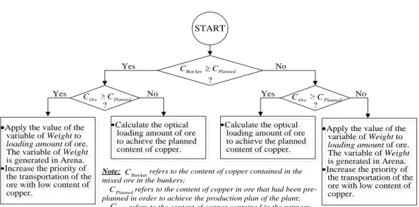
START ? Planned Ore C C ? Planned Bun C C ker ? Planned Ore C C

Calculate the optical loading amount of ore to achieve the planned content of copper.

Apply the value of the variable of Weight to loading amount of ore. The variable of Weight is generated in Arena. Increase the priority of

the transportation of the ore with low content of copper.

Apply the value of the variable of Weight to

loading amount of ore.

The variable of Weight is generated in Arena. Increase the priority of

Note: refers to the content of copper contained in the mixed ore in the bunkers;

refers to the content of copper in ore that had been pre-planned in order to achieve the production plan of the plant; refers to the content of copper contained in the primary ore. ker Bun C Planned C Ore C Yes No Yes No Yes No

Apply the value of the variable of Weight to loading amount of ore. The variable of Weight is generated in Arena. Increase the priority of

Apply the value of the variable of Weight to

loading amount of ore.

The variable of Weight is generated in Arena. Increase the priority of

Calculate the optical loading amount of ore to achieve the planned content of copper.

(7)

dispatch heuristic. Figure 4 presents an algorithm for calculating the optical loading amount when dispatching trucks to excavators. To illustrate this algorithm, for convenience, we provide a simple example. At the mining point Z, the content of copper contained in the ore is 0.60%. To maintain stable production in the enrichment plant, the ore must be stable and continuous at the averaged content of 0.53%. Thus far, 100 tons of ore have been transported to the bunker and the averaged copper content in the bunker is currently 0.48%. The question is how much ore with 0.6% copper content should be transported to the bunker? Here, the maximum load capacity of the truck is130 tons.

To solve the optimal transportation amount of 0.6% copper content ore (hereafter, Q), we generate a loop for Q from one ton to 130 tons with one-ton steps. While Q is looping, we calculate and estimate the copper content (hereafter, Cut%) after Q tons of 0.6%

ore content being fed to the bunker, and calculate the error between 0.53% and Cut%. Then, the Q yielding

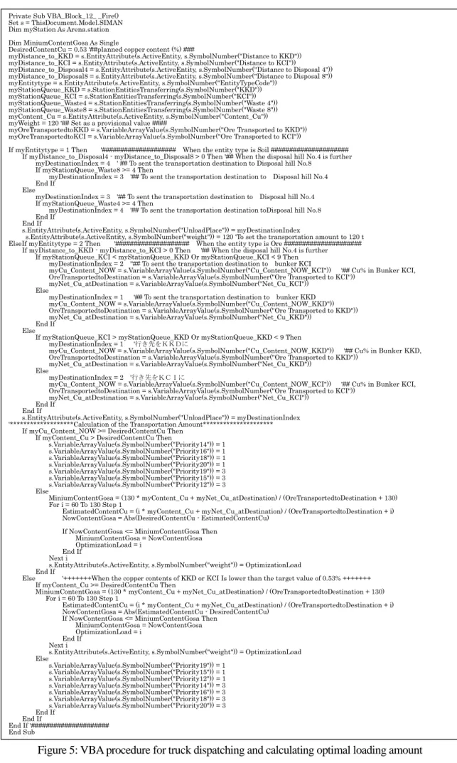
the smallest value of this error solves the problem. To verify the effectiveness of the proposed dynamic dispatch method, we revised the As-Is model

to another experimental model with Arena VBA programming. Figure 5 displays a section of this VBA procedure‟s code.

4.4 Simulation Experiment and Results

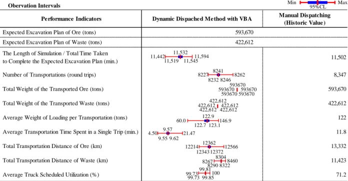
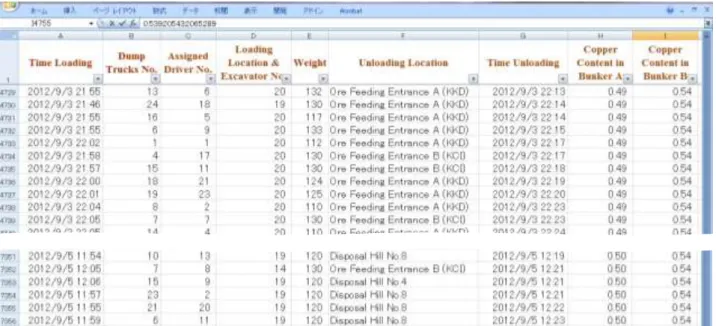
After building the simulation model, we validated it through an interactive process between the company staff and the modeler. This interactive process compared the model‟s output with the actual GPS tracking data. After confirming the model‟s reliability, we ran the simulations and analyzed the results. Table 3 displays the results of comparison between the manual and proposed VBA enhanced dynamic dispatch methods. Table 3‟s values are averaged execution results at the 95% confidence interval. We executed the simulation for 10 replications. Figure 6 presents a portion of the truck dispatch control table output by the VBA enhanced simulation model, which can be used to achieve the mining plan.

The results shown in Table 3 demonstrate that the VBA enhanced dynamic dispatch method improves the performance indicators‟ values. First, the simulation‟s duration, as well as the time taken to complete the

Table 3: Comparing results of manual dispatching and VBA enhanced dynamic dispatch method

Performance Indicators Dynamic Dispached Method with VBA Manual Dispatching (Historic Value) Expected Excavation Plan of Ore (tons)

Expected Excavation Plan of Waste (tons) The Length of Simulation / Total Time Taken

to Complete the Expected Excavation Plan (min.) 11,502

Number of Transportations (round trips) 8,347

Total Weight of the Transported Ore (tons) 593,670

Total Weight of the Transported Waste (tons) 422,612

Average Weight of Loading per Transportation (tons) 122

Average Transportation Time Spent in a Single Trip (min.) 11.8

Total Transportation Distance of Ore (km) 13,332

Total Transportation Distance of Waste (km) 11,423

Average Truck Scheduled Utilization (%) 71.2

593,670 422,612 Obervation Intervals Avg Max Min 95%CL 11,442 11,532 11,594 11,519 11,545 422,612 422,612 422,612 422,612 422,612 593670 593670 593670 593670 593670 9.57 21.47 4.50 9.55 9.62 100 99.7399.81 99.73 99.85 60.0 122.9 146.9 122.7 123.1 8241 8262 8227 8232 8246 12362 12566 12214 12343 12372 8460 8267 8304 8290 8322

(8)

Private Sub VBA_Block_12_ _Fire() Set s = ThisDocument.Model.SIMAN Dim myStation As Arena.station Dim MiniumContentGosa As Single

DesiredContentCu = 0.53 '##planned copper content (%) ###

myDistance_to_KKD = s.EntityAttribute(s.ActiveEntity, s.SymbolNumber("Distance to KKD")) myDistance_to_KCI = s.EntityAttribute(s.ActiveEntity, s.SymbolNumber("Distance to KCI"))

myDistance_to_Disposal4 = s.EntityAttribute(s.ActiveEntity, s.SymbolNumber("Distance to Disposal 4")) myDistance_to_Disposal8 = s.EntityAttribute(s.ActiveEntity, s.SymbolNumber("Distance to Disposal 8")) myEntitytype = s.EntityAttribute(s.ActiveEntity, s.SymbolNumber("EntityTypeCode"))

myStationQueue_KKD = s.StationEntitiesTransferring(s.SymbolNumber("KKD")) myStationQueue_KCI = s.StationEntitiesTransferring(s.SymbolNumber("KCI")) myStationQueue_Waste4 = s.StationEntitiesTransferring(s.SymbolNumber("Waste 4")) myStationQueue_Waste8 = s.StationEntitiesTransferring(s.SymbolNumber("Waste 8")) myContent_Cu = s.EntityAttribute(s.ActiveEntity, s.SymbolNumber("Content_Cu")) myWeight = 120 '## Set as a provisional value ####

myOreTransportedtoKKD = s.VariableArrayValue(s.SymbolNumber("Ore Transported to KKD")) myOreTransportedtoKCI = s.VariableArrayValue(s.SymbolNumber("Ore Transported to KCI"))

If myEntitytype = 1 Then '#################### When the entity type is Soil ##################### If myDistance_to_Disposal4 - myDistance_to_Disposal8 > 0 Then '## When the disposal hill No.4 is further myDestinationIndex = 4 ' ## To sent the transportation destination to Disposal hill No.8

If myStationQueue_Waste8 >= 4 Then

myDestinationIndex = 3 '## To sent the transportation destination to Disposal hill No.4 End If

Else

myDestinationIndex = 3 '## To sent the transportation destination to Disposal hill No.4 If myStationQueue_Waste4 >= 4 Then

myDestinationIndex = 4 '## To sent the transportation destination toDisposal hill No.8 End If

End If

s.EntityAttribute(s.ActiveEntity, s.SymbolNumber("UnloadPlace")) = myDestinationIndex

s.EntityAttribute(s.ActiveEntity, s.SymbolNumber("weight")) = 120 'To set the transportation amount to 120 t ElseIf myEntitytype = 2 Then '#################### When the entity type is Ore ##################### If myDistance_to_KKD - myDistance_to_KCI > 0 Then '## When the disposal hill No.4 is further If myStationQueue_KCI < myStationQueue_KKD Or myStationQueue_KCI < 9 Then myDestinationIndex = 2 ''## To sent the transportation destination to bunker KCI

myCu_Content_NOW = s.VariableArrayValue(s.SymbolNumber("Cu_Content_NOW_KCI")) '## Cu% in Bunker KCI, OreTransportedtoDestination = s.VariableArrayValue(s.SymbolNumber("Ore Transported to KCI"))

myNet_Cu_atDestination = s.VariableArrayValue(s.SymbolNumber("Net_Cu_KCI")) Else

myDestinationIndex = 1 '## To sent the transportation destination to bunker KKD myCu_Content_NOW = s.VariableArrayValue(s.SymbolNumber("Cu_Content_NOW_KKD")) OreTransportedtoDestination = s.VariableArrayValue(s.SymbolNumber("Ore Transported to KKD")) myNet_Cu_atDestination = s.VariableArrayValue(s.SymbolNumber("Net_Cu_KKD"))

End If Else

If myStationQueue_KCI > myStationQueue_KKD Or myStationQueue_KKD < 9 Then myDestinationIndex = 1 '行き先をＫＫＤに

myCu_Content_NOW = s.VariableArrayValue(s.SymbolNumber("Cu_Content_NOW_KKD")) '## Cu% in Bunker KKD, OreTransportedtoDestination = s.VariableArrayValue(s.SymbolNumber("Ore Transported to KKD"))

myNet_Cu_atDestination = s.VariableArrayValue(s.SymbolNumber("Net_Cu_KKD")) Else

myDestinationIndex = 2 '行き先をＫＣＩに

myCu_Content_NOW = s.VariableArrayValue(s.SymbolNumber("Cu_Content_NOW_KCI")) '## Cu% in Bunker KCI, OreTransportedtoDestination = s.VariableArrayValue(s.SymbolNumber("Ore Transported to KCI"))

myNet_Cu_atDestination = s.VariableArrayValue(s.SymbolNumber("Net_Cu_KCI")) End If

End If

s.EntityAttribute(s.ActiveEntity, s.SymbolNumber("UnloadPlace")) = myDestinationIndex '*******************Calculation of the Transportation Amount*********************

If myCu_Content_NOW >= DesiredContentCu Then

If myContent_Cu > DesiredContentCu Then s.VariableArrayValue(s.SymbolNumber("Priority14")) = 1 s.VariableArrayValue(s.SymbolNumber("Priority16")) = 1 s.VariableArrayValue(s.SymbolNumber("Priority18")) = 1 s.VariableArrayValue(s.SymbolNumber("Priority20")) = 1 s.VariableArrayValue(s.SymbolNumber("Priority19")) = 3 s.VariableArrayValue(s.SymbolNumber("Priority15")) = 3 s.VariableArrayValue(s.SymbolNumber("Priority12")) = 3 Else

MiniumContentGosa = (130 * myContent_Cu + myNet_Cu_atDestination) / (OreTransportedtoDestination + 130) For i = 60 To 130 Step 1

EstimatedContentCu = (i * myContent_Cu + myNet_Cu_atDestination) / (OreTransportedtoDestination + i) NowContentGosa = Abs(DesiredContentCu - EstimatedContentCu)

If NowContentGosa <= MiniumContentGosa Then MiniumContentGosa = NowContentGosa OptimizationLoad = i

End If Next i

s.EntityAttribute(s.ActiveEntity, s.SymbolNumber("weight")) = OptimizationLoad End If

Else '+++++++When the copper contents of KKD or KCI Is lower than the target value of 0.53% +++++++ If myContent_Cu >= DesiredContentCu Then

MiniumContentGosa = (130 * myContent_Cu + myNet_Cu_atDestination) / (OreTransportedtoDestination + 130) For i = 60 To 130 Step 1

EstimatedContentCu = (i * myContent_Cu + myNet_Cu_atDestination) / (OreTransportedtoDestination + i) NowContentGosa = Abs(EstimatedContentCu - DesiredContentCu)

If NowContentGosa <= MiniumContentGosa Then MiniumContentGosa = NowContentGosa OptimizationLoad = i

End If Next i

s.EntityAttribute(s.ActiveEntity, s.SymbolNumber("weight")) = OptimizationLoad Else s.VariableArrayValue(s.SymbolNumber("Priority19")) = 1 s.VariableArrayValue(s.SymbolNumber("Priority15")) = 1 s.VariableArrayValue(s.SymbolNumber("Priority12")) = 1 s.VariableArrayValue(s.SymbolNumber("Priority14")) = 3 s.VariableArrayValue(s.SymbolNumber("Priority16")) = 3 s.VariableArrayValue(s.SymbolNumber("Priority18")) = 3 s.VariableArrayValue(s.SymbolNumber("Priority20")) = 3 End If End If End If '##################### End Sub

(9)

Figure 6: Truck dispatching table output by VBA enhanced simulation model (partial)

expected mining plan, significantly decreased from 11,502 to 7,286 minutes. Thus, company A can use the time saved to expand their production. In addition, the total number of ore and waste transportation rounds and distances decrease. Because the trucks consume a large amount of gasoline, these transportation reductions will directly reduce transportation costs.

5 CONCLUSION

In this study, simulation models were constructed and enhanced with VBA programming to test and create a dynamic dispatch control table that satisfies an open pit mining plan. Results demonstrated that by combining the simulation technique with Excel and VBA programming, trucks‟ transportation performance could be significantly improved, thus reducing transportation costs. Simulations can help mining project managers understand the system‟s behavior by providing visual and dynamic descriptions, allowing them to optimize the system through appropriate strategies.

ACKNOWLEDGMENTS

This research was supported by the Grant-in-Aid for Asian CORE Program "Manufacturing and Environmental Management in East Asia" of Japan Society for the Promotion of Science (JSPS).

REFERENCES

Alarie, S. and M. Gamache. (2002) “Overview of solution strategies used in truck dispatching systems for open pit mines,” International Journal of Surface Mining, Reclamation and Environment, Vol.16, pp.9-76.

Bauer, A., and P. N. Calder. (1973) “Planning Open pit Mining Operations Using Simulation,” In APCOM 1973, pp.273-298. Johannesburg: South Africa Institute of Mining and Metallurgy.

Beaulieu, M and M., Gamache. (2006) “An enumeration algorithm for solving the fleet management problem in underground mines,” Computers and Operations Research, Vol.33, No.6, pp.1606-1624.

Biles, W. E. and J. K. Bilbrey. (2004) “Integration of Simulation and Geographic Information Systems: Modeling Traffic Flow on Inland Waterways,” In

Proceedings of the 2004 Winter Simulation Conference, ed. R. G. Ingalls, M. D. Rossetti, J. S. Smith, and H. A. Peters, pp.1392-1398. Piscataway, New Jersey: Institute of Electrical and Electronics Engineers, Inc.

Boland, N., I. Dumitrescu, G. Froyland, and A. M. Gleixner. (2009) “LP-based Disaggregation Approaches to Solving the Open pit Mining Production Scheduling Problem With Block Processing Selectivity,” Computers & Operations Research, Vol.36, pp.1064-1089.

(10)

Burt, C., L. Caccetta, S. Hill, and P. Welgama. (2005) “Models for Mining Equipment Selection,” In

Proceedings of MODSIM 2005 International Congress on Modelling and Simulation, ed. Zerger, A., and R. M. Argent, pp.170-176.

Chinbat, U. and S. Takakuwa. (2009) “Using Simulation Analysis for Mining Project Risk Management.” In

Proceedings of the 2009 Winter Simulation Conference, ed. M. D. Rossetti, R. R. Hill, B. Johansson, A. Dunkin and R. G. Ingalls, pp.2612–2623. Piscataway, New Jersey: Institute of Electrical and Electronics Engineers, Inc.

Ercelebi, S. G. and A. Bascetin. (2009) “Optimization of shovel-truck system for surface mining,” Journal of the Southern African Institute of Mining and Metallurgy,

Vol.109, pp.433-439.

Fioroni, M. M., L. A. G. Franzese, T. J. Bianchi, L. Ezawa, L. R. Pinto, de Miranda, and J. Gilberto. (2008) “Concurrent Simulation and Optimization Models for Mining Planning.” In Proceedings of the 2008 on Winter Simulation Conference, ed. S. J. Mason, R. R. Hill, L. Moench, O. Rose, pp.759-767. Piscataway, New Jersey: Institute of Electrical and Electronics Engineers, Inc. Kelton, D., R. Sadowski, and N. B. Swets. (2010) Simulation

with Arena. 5th Edition. New York: McGraw-Hill, Inc. Kolojna, B., D. R. Kalasky, and J. M. Mutmansky. (1993)

“Optimization of dispatching criteria for open pit truck haulage system design using multiple comparisons with the best and common random numbers,” In Proceedings of the 1993 Winter Simulation Conference, ed. G. W. Evans, M. Mollaghasemi,. E.C. Russell,. W.E. Biles., pp.393-401. Piscataway, New Jersey: Institute of Electrical and Electronics Engineers, Inc.

Miwa, K. and S. Takakuwa (2005) “Flexible module-based modeling and analysis for large-scale transportation-inventory systems,” In Proceedings of the 2005 Winter Simulation Conference, ed. M.E. Kuhl, N.M. Steiger, F.B. Armstrong, and J.A. Joines, pp.1749-1758.

Piscataway, New Jersey: Institute of Electrical and Electronics Engineers, Inc.

Neonen, L. K., P. W. U. Graefe, and A. W. Chan. (1981) “Interactive computer model for truck/shovel operations in an open pit mine,” In Proceedings of the 1981 Winter Simulation Conference, ed. T.I. Oren, C.M. Delfosse, C.M. Shub, pp.133–139. Piscataway, New Jersey: Institute of Electrical and Electronics Engineers, Inc. Qing-Xia, Y. (1982) “Computer simulation of drill-rig/shovel

operations in open pit mines,” In Proceedings of the 1982 Winter Simulation Conference, ed. H. J. Highland, Y. W. Chao, and O. S. Madrigal, pp.463-468. Piscataway, New Jersey: Institute of Electrical and Electronics Engineers, Inc.

Seppanen, M.S. (2000) “Developing Industrial Strength Simulation Models Using Visual Basic for Applications (VBA)”, In Proceedings of the 2000 Winter Simulation Conference, ed. J.A. Joines, R.R. Barton, K. Kang, and P.A. Fishwick, pp.77–82. Piscataway, New Jersey: Institute of Electrical and Electronics Engineers, Inc. Song, L., F. Ramos, and K. Arnold. (2008) “A Framework

for Real-Time Simulation Of Heavy Construction Operations,” In Proceedings of the 2008 Winter Simulation Conference, ed. S. J. Mason, R. R. Hill, L. Monch, O. Rose, T. Jefferson, And J. W. Fowler, pp..2387-2395. Piscataway, New Jersey: Institute of Electrical and Electronics Engineers, Inc.

Subtil, R. F., D. M., Silva, and J. C., Alves. (2011) “A Practical Approach to Truck Dispatch for Open pit Mines,” 35Th APCOM symposium, pp.765-777.

Tan, Y. and S. Takakuwa (2012) “Operations Modeling and Analysis of Open Pit Copper Mining Using GPS Tracking Data,” to the published in Proceedings of the 2008 Winter Simulation Conference, ed. C. Laroque, J. Himmelspach, R. Pasupathy, O. Rose, and A.M. Uhrmacher. Piscataway, New Jersey: Institute of Electrical and Electronics Engineers, Inc. (Accepted in July 2012)