Large-Scale Evolutionary Optimization Using Multi-Layer Strategy Differential Evolution

(1)

LARGE-SCALE EVOLUTIONARY OPTIMIZATION

USING MULTI-LAYER STRATEGY DIFFERENTIAL

EVOLUTION

By: Tarik Eltaeib

Under the Supervision of Prof. Ausif Mahmood

DISSERTATION

SUBMITTED IN PARTIAL FULFILMENT OF THE REQUIRMENTS FOR THE DEGREE OF DOCTOR OF PHILOSOHPY IN COMPUTER SCIENCE

AND ENGINEERING THE SCHOOL OF ENGINEERING

UNIVERSITY OF BRIDGEPORT CONNECTICUT

(2)

(3)

iii

LARGE-SCALE EVOLUTIONARY OPTIMIZATION USING

MULTI-LAYER STRATEGY DIFFERENTIAL EVOLUTION

(4)

iv

LARGE-SCALE EVOLUTIONARY OPTIMIZATION USING

MULTI-LAYER STRATEGY DIFFERENTIAL EVOLUTION

ABSTRACT

Differential evolution (DE) has been extensively used in optimization studies since its development in 1995 because of its reputation as an effective global optimizer. DE is a population-based metaheuristic technique that develops numerical vectors to solve optimization problems. DE strategies have a significant impact on DE performance and play a vital role in achieving stochastic global optimization. However, DE is highly dependent on the control parameters involved. In practice, the fine-tuning of these parameters is not always easy. Here, we discuss the improvements and developments that have been made to DE algorithms.

The Multi-Layer Strategies Differential Evolution (MLSDE) algorithm, which finds optimal solutions for large scale problems. To solve large scale problems were grouped different strategies together and applied them to date set. Furthermore, these strategies were applied to selected vectors to strengthen the exploration ability of the algorithm. Extensive computational analysis was also carried out to evaluate the performance of the proposed algorithm on a set of well-known CEC 2015 benchmark

(5)

v

functions. This benchmark was utilized for the assessment and performance evaluation of the proposed algorithm.

(6)

vi

ACKNOWLEDGEMENTS

Special appreciations to my family. Words cannot express how thankful I am to my wife, my daughters, my mother, my mother-in law, and father-in-law for all of the sacrifices and prayers for me that you’ve made on my behalf. I would like to express my special thanks to my advisor Professor Ausif Mahmood and his efforts, encouraging and guiding me to grow as a research scientist.

(7)

vii

LIST OF TABLES

Table 1.1 The differentiation operation can be carried out using many mutation strategies.

18

Table 2.1 Summary of different DE algorithms with verity of approaches.

50

Table 4.1 Mean experimental results for 30 Variables over 50 runs 59

Table 4.2 Mean experimental results for 100 Variables. 61

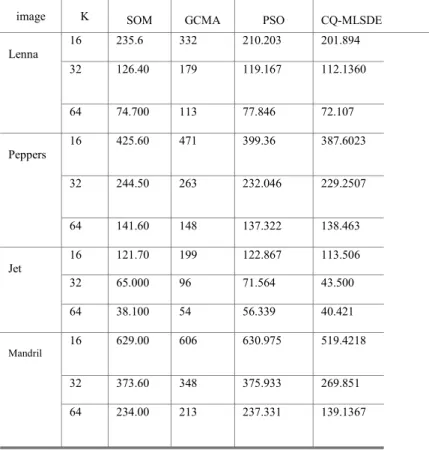
Table 5.1 The MSDE was tested with quantization of lenna, pepper, jet and mandrill images.

(10)

x

LIST OF FIGURES

Figure 1.1 Random vectors selected in the mutation strategy (classic DE)

15

Figure 1.2 The differential β and base vector δ provide the optimal direction

18

Figure 3.1 The flowchart of Proposed MLSDE 56

Figure 4.1 Comparing between MLSDE, JADE, JDE, and SADE 59

Figure 4.2 Experimental Results for 100 Variables 61

Figure 5.1 Generating a digital image and Continuous image 64 Figure 5.2 Generating a digital image Sampling and quantization 65

Figure 5.4 Quantization result of images 68

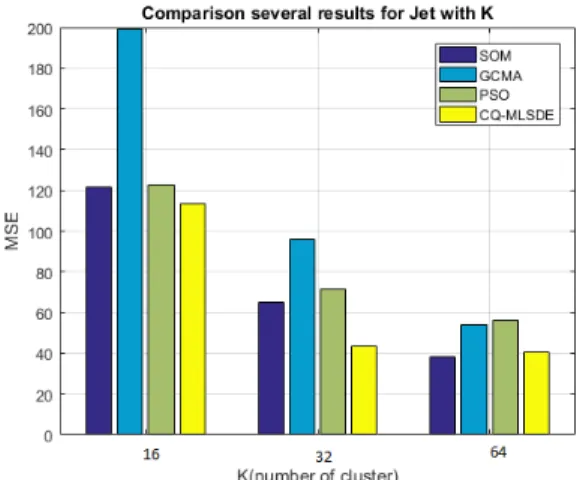
Figure 5.5 Experimental results Jet 77

Figure 5.6 Experimental results Lenna 77

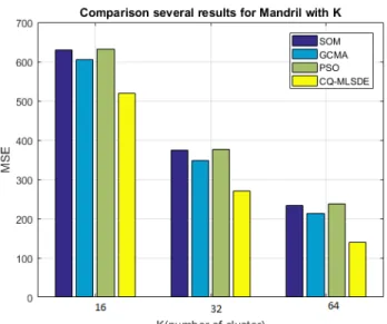
Figure 5.7 Experimental results Mandril 78

(11)

CHAPTER 1: INTRODUCTION

1.1 Background

Optimization algorithms are important approaches for resolving hard optimization problems [1]. Optimization is defined as the procedure of discovery that provides the minimum or maximum value of a function f(x) [2, 3]. There are many reasons that make this problem difficult to solve. First, we cannot perform a comprehensive search if the problem domain space is too large. Second, the evaluation function is noisy or varies with time, generating a series of solutions instead of a single solution. Third, sometimes the constraints prevent arriving at a possible solution such that the optimization approach is the only solution [4].

Differential evolution (DE) is a stochastic algorithm for solving numerical continuous optimization problems. Since its inception, the DE algorithm has been a powerful global optimizer. DE was developed by Kenneth Price in 1994 and has since become a promising optimization algorithm that converges to the real optimum without using significant amounts of resources. Furthermore, its performance was validated in the evolutionary domain by the IEEE Conference on Evolutionary in 1996 [5].

More recently, different versions of DE have secured the top ranks in many competitions between evolutionary algorithms (EAs) by the IEEE Congress on

(12)

12

Evolutionary Computation (CEC) conference series (http://www.ntu.edu.sg/home/epnsugan/index_files/cec- benchmarking.htm).

1.2. Research Problem and Scope

An impressive number of different DE algorithms have been introduced by the research community over the past decades because various DE algorithms involving different techniques. To differentiate among those techniques, we need to define a comprehensive framework that helps to deepen understanding of the characteristics of different DE strategies, with the goal of benefiting from the various approaches. In fact, understanding how to combine these DEs harmoniously and their underlying concepts could be crucial to attaining effective designs or improving the performance of DE algorithms in particular or any optimization algorithms in general. Moreover, the literature shows that no single algorithm has been demonstrated to be effective for various applications.

DE algorithms are different from EA algorithms that shape offspring by mixing solutions with a difference factor rate of selected individual vectors and are an alternative to recombining individuals through a probabilistic scheme. In fact, the differential mutation strategy is the main component that distinguishes DE from other population algorithms. Applying the mutation to all candidates defines an exploration rule based on other candidate solutions. Therefore, the mutation strategy enhances a population’s capability for discovering new promising offspring based on the current distribution of solutions within the domain space. Ideally, the performance of DE is based on two major

(13)

13

components: the chosen strategy and the control parameters. However, the strategy underlying DE consists of mutation, crossover and selection operators, which are utilized at each generation to determine the global optimum. The control parameter components consist of the population size NP, scaling factor F and the crossover rate Cr.

1.3. Motivation behind the Research

Despite the potential of DE, it is obvious to the research community that some adjustments to classic DE are essential to significantly enhance its performance, especially in addressing high-dimension problems. Stagnation, premature, convergence, and sensitivity are the control parameters that influence the performance of DE. To evaluate the reliability and robustness of the different DE algorithms, we introduce a general framework that includes the control parameters for evaluating the efficiency of the different algorithms. For example, stagnation occurs when the population cannot converge to a suboptimal solution although the diversity of the population remains high. This does not improve the population over a period of iterations, and the algorithm is not capable of finding a new search domain. There are many causes of stagnation, including control parameters that become inefficient for a specific problem in the decision space. Many studies have proposed a variety of ways to improve the current DE algorithm through modifications, including the use of differential mutations with perturbations, mutations with selection pressure, and operator adaption techniques. To address this need, we have conducted an extensive study on differential evolution and observed that

(14)

14

the performance of differential evolution and the quality of the results are based on the type of technique used, and what control parameters are effective.

1.4. Potential Contribution of the Proposed Research

We propose a Multi-Layer Strategies Differential Evolution (MLDE) approach, which uses different mutation strategies in order to reach a fast convergence rate and avoid premature convergence due to the loss of diversity in the population. In fact, we used multilayer crossover techniques since there no single method has proven fit for every problem; though a crossover scheme may work perfectly with some problems, they may perform poorly with others. Each problem has different characteristics: some research showed that a scheme such as binomial crossover performed well with some type of problem. MLDE works to improve the diversification of offspring by using different strategies in a multiple-layer approach. This approach makes the population widely spread so the sampled vectors can easily generate better new offspring. This technique can accelerate convergence rate for finding the optimum solution with a smaller number of iterations.

Another significant factor is considered in this work is to provide a comprehensive study of the different types of state-of-the-art differential evolution algorithms that are available as global numerical optimizations in continuous search space. This comprehensive study sheds light on most improvements and developments pertaining to different types of DE families, including primary concepts and a variety of DE formats.

(15)

15 1.5 Literature Survey and Background

1.5.1 Classic Differential Evolution

If we are seeking the optimum for X* which demonstrate by vector ,i=1,…D , X , within boundary constraints L ≤ X ≤ H. Differential evolution (DE) is population-based, where the initial population with random initialization . Initialization of the population is important step that assuming that there is no previous information about the optimum solution. Therefore, the population is initialized within only boundary constraints upper bound (H) and lower bound (L), so the population can by initialized by the following

After the initialization phase, the evolution involves the three processes of mutation, crossover, and selection. The classic differential evolution strategy consists of three random vectors , and that are selected from the population (Eq. 1). Randomly select of three individuals from the population

≠

while (

The mutation operation recombines to construct the mutation vector shown in Figure 1. The associated equation.

(16)

16

Figure 1.1 Random vectors selected in the mutation strategy (classic DE)

The mutation process is the main distinctive component of DE and is considered the strategy by which DE is carried out. There are different types of mutation strategies, each one distinguished with an abbreviation based on the classic mutation strategy described by equation (1), i.e., DE/rand/1/bin, where DE represents differential evolution and “rand” represents random, which indicates that the vectors are selected randomly. The number one indicates the number of difference pairs; in this strategy, it is one pair . The last term represents the type of crossover used. This term could be “exp,” for exponential, or “bin,” for binomial [9]. Then, to complement the previous step (mutation strategy), DE also apply uniform crossover to construct trial vectors which is out of parameter values that have been copied from two different vectors. In particular, DE selected random vector from population indicate as which must be different of , and ; and then it crosses with a mutant vector ; the binomial crossover is generated as follows:

(17)

17

= (1.2)

The crossover probability, Cr ∈ (0, 1), is a pre-defined rate that specify the fraction of parameter that are transferred from the mutant. Thus, it use to control which source participate a given parameter. Uniform crossover rate compares with uniform random values form from rand (0,1); if the random value is smaller than or equal to Cr then the trial parameter is copied from mutant vector else the parameter is inherited from

The next operation is selection, in which the trail vector competes with the target vector . If this trail vector is equal or less than it changes the target vector in the next generation else not changed in the population

=

Where is the objective function? Therefore, if the new trail vector

is less than or equal to the target vector , it replaces the target vector. Otherwise, the population maintains the target vector value. Therefore, the different DE phases prevent the population from ever deteriorating; the population either remains the same or improves. Furthermore, continued refining of the population is updated by the trial vector, although the fitness of the trial vector is the same as that of the current vector. This factor is crucial in DE because it provides the algorithm the ability to move through the landscape using a variety of generations [10]. The termination condition can be either a preset maximum number of generations or a pre-specified target of the objective function value. [11].

(18)

18

1.5.2 Differential Evolution Strategies

Table (1.1) The differentiation operation can be carried out using many mutation strategies.

Strategy Formulation 1. DE/best/1/exp 2. DE/rand-to-best/1/exp 3. DE/best/2/exp 4. DE/rand/2/exp 5. DE/best/1/bin 6. DE/rand/1/bin 7. DE/rand-to-best/1/bin 8. DE/best/2/bin 9. DE/rand/2/bin

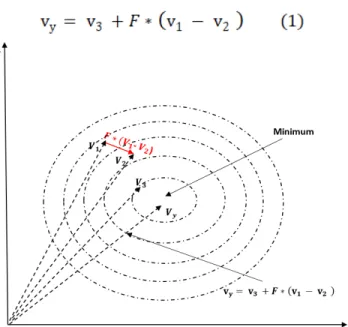
The various equations underpinning DE possess certain aspects in common when applied for continuous optimization. All consist of an original point sometimes referred to as the base point. The original algorithm carries out the search operation such that it finds the optimum as soon as possible. We can generalize the DE formula to the form α = β + F · δ, where β represents the base vectors and δ the difference between vectors. Thus, the main goal of all DE equations is to provide the optimal direction based on the differential β and base vector δ (Figure 2).

(19)

19 Y-Ax is X-Axis β δ

Figure 1.2 The differential β and base vector δ provide the optimal direction

Establishing β and δ is crucial to creating an efficient strategy that can be applied to the chosen individuals from the population. However, all possible combinations of β and δ can be classified into the following strategies: local, random, directed, and hybrid. In random strategies, abbreviated as “Rand”, all individuals are formed randomly, and there is no prior information about the objective function. In directed strategies, abbreviated as “DIR”, a suitable value for the base vector is chosen according to the objective function to ensure a suitable direction. Hybrid strategies include the combination of “Rand” and “DIR”, labeled RAND/DIR. In another approach, the best overall vector is used, not only the best among the selected individuals; this approach is referred to as the “BEST”. Combining the “Rand” and “BEST” yields the hybrid RAND/BEST strategy. In addition, the combination of more than two approaches, e.g., RAND/BEST/DIR, can yield favorable results by exploiting the advantages of each approach.

(20)

20

However, Table 3.1 shows that all DE strategies employed are formed based one the DE/rand/x variation, which applies pairs of difference vectors:

whereas the scaling factors are frequently presumed to be the same F1 = F2 =… = Fk = F. Substituting an arbitrary base vector 𝐱𝐱1 as vbest, “the best vector” from the population, provides a different DE approach, indicated DE/best/1:

Most mutation strategies can be formed by a general formula based on the sum of k scaled difference vectors and a weighted average among the best vector and arbitrary ones:

One aspect common to all the mutation strategy methods is the base vector, which controls the search direction. The difference vector provides a mutation rate term, such as a self-adaptive term, that is added to an arbitrary or guided base vector to construct a trial individual. Over generations, the individuals of a population reside in increasingly better positions and reform themselves. The various combinations of these vectors can be categorized into four groups based on information pertaining to the values gathered from the objective function: random, directed, local and hybrid.

The RAND approach consists of strategies in which the trial individual is produced without knowledge of the value of the objective function. Similarly, the RAND/DIR approach includes strategies that use the values of the objective function to determine a promising direction. Likewise, the RAND/BEST approach applies the best

(21)

21

individual approach to proceed with a trial. Additionally, the RAND/BEST/DIR approach combines the last two groups into one that includes all of their collective benefits.

However, a suitable direction is obtained by using the best individual to decrease the search space and exploration time [12, 13]. Thus, the “dir” and “dir-best” strategies, which use objective function values to generate trial individuals, can produce an exploitation function. In fact, the random selection of parents for a trial enhances exploration capabilities [14-16]. Thus, the locations of individuals carry information about the fitness landscape. Therefore, an effective mutation strategy that leads to uniform random vectors represents the entire search space well.

1.5.3 Initialization

DE is a population-based optimization technique that begins with the problem solution by selecting the objective function at a random initial population. Predefined parameter bounds describe the area from which the number of population (Np) vectors in this initial population is chosen within both the upper bound “ ” and the lower bound “ ”, where the subscripts L and U indicate lower and upper, respectively. The following equation is used to develop a random number generator for all vectors from within the predefined upper and lower bounds. The random function Random(0, 1) outputs a uniform random number within the range (0, 1).

(22)

22 1.5.4 Crossover

To balance the differential mutation search strategy, DE also applies uniform crossover to construct trial vectors. A trial vector is constructed from values that have been copied from two diverse vectors. In particular, DE crosses each vector as follows:

The crossover probability, ∈ [0,1], is predefined in the classic version of DE, and the fraction value of the Cr control is cloned from the mutant vector. is compared with a random number randj(0,1). If the random number is less than or equal to , the trial parameter is inherited from the mutant otherwise, the parameter is cloned from the vector .

1.5.5 Selection

In this stage, we determine when the trial vector has an objective function value that is less than or equal to that of its target vector . DE swaps the target vector in the next iteration; otherwise, the target retains its place in the population. This process is carried out by comparing each trial vector with the target vector from which the parameters are cloned. After the population is updated, mutation, recombination and selection are repeated until the optimum value is found or after a predefined stop criterion is reached, such as a certain number of iterations.

If (

(23)

23

1.5.6 DE Applications and related automated

Due to the rapid rise of DE as a modest and strong optimizer, developers have applied the technique in a wide range of domains and fields of technology1. Yalcin proposed a new method for the 3D tracking of license plates from video using a DE algorithm, which could be fine-tuned according to the license plate boundaries [17]. A color image quantization application using DE was proposed by Qinghua and Hu. The main objective of image processing techniques is to, during the color image quantization phase, decrease the number of colors in an image with a low amount of deformation. DE can be used to adjust colormaps and find the optimal candidate colormap [18]. With respect to the bidding market, Alvaro et al. applied DE in developing a competitive electricity market application that finds the optimal bids based on daily bidding activity [19]. Sickel et al. used DE in developing a power plant control application for a reference governor to produce an optimal group of points for controlling a power plant that was produced by [20]. Wang et al. proposed a flexible QoS multicast routing algorithm for the next-generation Internet that improves the quality of service (QoS) of multicasts to manage the increasing demand of network resources [21]. With respect to the electric power systems industry, Ela et al. applied DE to determine the optimal power flow [22]. Goswami et al. proposed a DE application for model-based well log-data inversion to

1_{http://www1.icsi.berkeley.edu/~storn/code.html}

If (

(24)

24

discover features of earth formations based on the dimensions of physical phenomena [23]. Another application applies network system reconfiguration for distributing systems. The network reconfiguration application proposed by Tzong and Lee involves the application of Improved Mixed-Integer Hybrid Differential Evolution [24]. Another DE application developed by Boughari et al. sets suitable controllers for aircraft stability and control augmentation systems [25].

1.5.7 Parameter Control

The DE algorithm is a simple and effective optimization algorithm for problems from real world when its control parameters are suitably set [8, 26, 27], as reviewed in the previous section. In this section, we review the most current improvement approaches for DE. First, the DE algorithm applies certain control parameters to the system implementation. The accomplishment of DE is influenced by the value of parameters, such as the crossover and mutation rate. Although some studies have recommended certain values for these parameters, their effect on performance is complex and their exact values are unclear. In particular, there is a wide variety of different recommended values that are appropriate for different problems [28-30].

The mutation rate ”, crossover rate “ and population dimension maintain balance between exploration and exploitation [6]. Exploration is associated with finding new solutions, and exploitation is associated with searching for new suitable solutions; the two processes are linked in the evolutionary search [31, 32]. Therefore, the mutation and crossover rates influenced the convergence rate and the effectiveness of the search space [33].

(25)

25

However, specifying suitable values for these rates is not easy [34]. Three types of strategies are used to set these parameter controls: deterministic parameter control (sometimes called random), self-adaptive parameter control and adaptive parameter control [10, 35-37]. Adaptive and self-adaptive parameter control [9-14, 38-41] have recently been proposed to dynamically alter the control parameters without requiring the user’s prior knowledge or information about the problem behaviors throughout the search process [42-46]. In the following sections, the self-adaptive parameter, the adaptive parameter, and hybrid control strategies are discussed.

1.5.8 Deterministic Parameter Control

The parameters are altered using a deterministic rule regardless of the feedback from the evolutionary search, with Jitter and Dither being two operators that are used in this technique. Dither scales the distance of the vector differentials as the same factor, , is applied to all the elements of a subtracted vector. Jitter multiplies each vector element of the subtracted vector by a different scale factor, . The rotation creates jitter using an essentially different procedure than the classic DE’s constant mutation with F. However, this approach shows robustness for non-deceiving objective functions [3]. Nonetheless ,applied fixed values for each iteration, and F was created for each individual within the range [0.4, 1] range, whereas the interval [0.5, 0.7] was selected for Cr [47, 48].

Another approach is the composite DE (CoDE) algorithm proposed by Wang et al. In CoDE, a trial vector is selected from a set of groups produced by utilizing diverse DE strategies [49]. The main objective is to arbitrarily merge many trial vector strategies with different parameter at each iteration to construct new trial vectors. These

(26)

26

combinations help solve many problems successfully. Wang et al. used group of trial vector strategies and group of control parameter (almost three) to create strategy and parameter candidate pools. The selected strategies are DE/rand/1/bin, DE/rand/2/bin and DE/current-to- rand/1, and the three pair common choices for the control parameter settings were (F= 1.0, Cr =0.1), (F =1.0; Cr=0.9), and (F =0.8; Cr=0.2). In each generation, the three different strategies are applied, which randomly pick any of the control parameter values.

Then, the trial vector is designated the candidate with the better value of fitnes. The parameters are chosen based on whether they are frequently implemented with many DEs, and their performances are evaluated. The three pairs of parameter settings that provide diverse effects produce new improved candidates. Furthermore, the different values of the control parameters maintain different levels of search performance.

1.5.9 Adaptive Parameter Control

The adaptive technique has been applied with classic DE/rand/1/bin; while the performance is relatively favorable, the technique still suffers from convergence rate issues [43, 44]. Very good designed a self-adaptive and adaptive parameter controls can enhance the robustness and the convergence rate by automatic adapting to the parameters. Approaches other than using the best explored solution use minor resolution in previous generations and their variation with the present population as a good area for finding the optimum. Adapting the parameters is a method called the adaptive DE algorithm (ADE), which applies a adapting evaluation from feedback of F relay on additional parameter (ϒ) that necessity be adjusted[50, 51]. However, the self-adaptive parameter controls the

(27)

27

value assignments and adjusts them dynamically. A parameter is altered dynamically through processing according to pre-defined rules using adaptive control, self-adaptive control or a combination thereof [34, 52]. In addition, the self-adaptive parameter control mix explores the optimal parameter values with the goal of finding the optimal solutions. Indeed the adaptive approach have been achieved success with different technologies; Shojafar et al., 2016 applied the adaptive technique within cloud in order to reach the communication optimization framework and exploiting virtualization technologies[53, 54].

The main purpose of adaptive DE is to help exploit and explore relationships that avoid premature convergence problems and to optimize the final results. In general, there are many techniques for hybridizing a conventional evolutionary algorithm to solve optimization problems. The initial population of DE is formed by problem-specific heuristics. Then, other solutions obtained using another EA might be enhanced with a local search. This type of combination is called a memetic algorithm [10, 52]. The benefits of this hybridization lead to various operators that might exploit problem knowledge, such as merging more promising individuals to be inherited. Furthermore mutation operations may be biased to contain solutions of promising individuals with higher probabilities than those of others.

1.5.10 Differential Evolution with Self-Adapting Populations (DESAP) Differential Evolution with Self-Adapting Populations (DESAP) dynamically adjusts the crossover and mutation parameters δ , η and the population size π [39]. Each individual is connected to its control , , and . δ and π have similar meanings to NP

(28)

28

and CR correspondingly. The mutation factor F is retained as static, and η denotes the probability of implementing an extra mutation using normally distributed after crossover. The main technique of DESAP is unlike that of the traditional DE/rand/1/bin algorithm [38]. Parameters are adapted by developing them over the mutation and crossover processes, as the procedures are applied to each . The updated values of that parameters continue with if . However, DESAP still requires further development to produce better performance. In fact, despite its simplicity, DESAP performs better than DE in one of De Jong’s five exam problems, whereas the other solutions are very identical. DESAP represents an opportunity to reduce the control parameters further by updating the size of population, as is done with the additional parameters.

1.5.11 Fuzzy Adaptive Differential Evolution (FADE)

Fuzzy adaptive differential evolution (FADE), presented by Lampinen and Liu [41], is a different type of DE algorithm that apply fuzzy logic controllers to adjust the controller parameters and for the crossover and mutation operations. Similarly to DESAP, the size of the population is presumed to be adjusted and is static during the evolution procedure [9]. The fuzzy-logic control method has been verified on a group of 10 functions as benchmark and displays best solutions than those of classic DE for high-dimensional problems.

(29)

29

1.5.12 Self-adaptive Differential Evolution (SaDE)

Self-adaptive Differential Evolution (SaDE) is simultaneously applied to pair of mutation techniques “DE/rand/1” and “DE/current-to-best/2” [45]. The adaptation technique of parameter consists of two chunks: the probability of the adaptation , where

= (1, 2), and the DE parameters and . The probability of producing a mutation vector based on the two strategies approaches 0.5 and is updated every 50 iterations using the following method:

where and are the numbers of offspring vectors constructed by the i = (1, 2) strategy that was a success or failure in the selection process over the last 50 generations. It is assumed that this adaptation process can progressively develop the most appropriate mutation strategy at diverse learning phases for a given problem. The mutation factors are autonomously created at each iteration based on a normal distribution ”NR” with a mean of 0.5 and a standard deviation of 0.3,

= NR(0.5, 0.3)

The crossover rates are autonomously formed based on a normal distribution with a mean of and a standard deviation of 0.1. The mean approaches 0.5, is changed every 25 iterations and is set to be the mean of the effective Cr over the previous 25 generations.

(30)

30

where K is the counters of effective Cr values and indicates the value.To accelerate the convergence, a local search technique (Quasi–Newton method) is applied to respectable individuals after 200 generations. SaDE has been further developed by applying five mutation strategies to resolve a group of constrained problems [55].

One of the success fuzzy application that applied on cloud computing which consists of numerous of computers linked over instantly transmission network, so it provides the capability to instantaneously perform an numerous software on connected workstations. The job scheduling is one of vital and interesting aspects in cloud computing. FUGE based on fuzzy theory and genetic algorithm that assign jobs to resources optimally considering execution time and cost(memory, virtual machine speed, network rate, and job intervals) .Applied fuzzy theory with modified the standard genetic algorithm (SGA) and used to invention a fuzzy-based steady-state GA. In this approach, jobs are denoted as genes and resources of computing allocated to these genes, and groups of genes produce chromosomes. They created two different forms of chromosomes: first type is based on job length, CPU speed and size of the resources and another form is rely on job length and bandwidth of resources. For each type of chromosome, population of genes are randomly created and computational resources are assigned to gene randomly. Algorithm calculates the value of fitness for each chromosome using a fuzzy function. Fuzzy theory is also used in the crossover step of the GA. In general, single point or two point crossover are used in crossover approach, but in this approach, fuzzy-based crossover that is one of the new approach [56].

(31)

31 1.5.13 Self-adaptive NSDE (SaNSDE)

Neighborhood search differential evolution (NSDE) is similar to classic DE except that Eq. (1) which is replaced with

where is the differential deviation, N (0.5,0.5) means a Gaussian random number with a average of 0.5 and a standard deviation of 0.5 and δ indicte a Cauchy random variable with a rate parameter of t=1.

Self-adaptive DE (SaDE) [8] was developed to resolve the control parameters and learning technique . In SaDE, two DE learning strategies are chosen according to their performance. The most appropriate learning technique and parameter values are increasingly self-adapted according to the learning experience gained during evolution [57].

SaNSDE is an adaptive differential evolution algorithm that produces mutation vectors in a manner similar to SaDE [57]. However, the difference is that the mutation factors are established based on a normal distribution or a Cauchy distribution:

where the normal distribution (μ, ) indicates a random value of mean μ and variance and a (μ, δ) indicates a random value with scale parameters μ and δ. The probability of the spread over is adapted as follows.

(32)

32

.

The crossover rate adaptation is similar to the method used in SaDE, but the factor is changed as a biased average of the successful values every 25 iterations.

where the weight is calculated with a positive improvement = f (x) – f (u) in the selection related to each successful crossover rate CRsuc(k).

1.5.14 Self-Adapting Parameter Setting in Differential Evolution (jDE) jDE is another adaptive DE algorithm that is similar to the classic DE/rand/1/bin algorithm. jDE improves the population size throughout the optimization process based on the improved parameters and thus generates vectors that are more likely to survive. However, the mechanism of jDE involves adapting the parameters Fi and CRi associated with each individual. At the beginning of the process, the parameter values are Fi = 0.5 and CRi = 0.9 for each individual. However, Fi and CRm are updated from the effective records; thus, jDE produces new values within the probabilities = , which are used to alter the control parameters. The updated values for Fi and CRi are then obtained using uniform distributions over [0.1, 1] and [0, 1], respectively. That is,

(33)

33

where j = 1, 2, 3, 4 is the uniform random function ∈[0, 1]. The updated parameters are implemented in the mutation and crossover processes to produce new, consistent vectors. This mechanism updates the prior parameter with a new one only if the new vectors pass the selection phase. However, jDE yields improved results with the classic DE/rand/1/ bin strategy.

1.5.15 Adaptive DE algorithm (ADE)

Hu and Yan proposed another adaptive DE algorithm. They modified the parameters F and Cr to each iteration using the current generation and the fitness [58]. They tried to find the optimal value for the parameters F and Cr to find a balance between reliability and efficiency. The mutation and crossover operations are calculated for each generation. Thus, for each parent of generation g, the offspring is constructed as follows: calculate the mutation and crossover as

(34)

34 1.5.16 Modified DE (MDE)

MDE uses only one array, which is updated when a better solution is found. Therefore, continuously updating the one array improves the convergence speed, leading to fewer evaluation procedures than those associated with classical DE [59]. In MDE, and by applied distribution of Laplace “F” is arbitrarily adjusted [59]. The Laplace distribution is analogous to the (NP) Normal Distribution [60]. Moreover, the Laplace has a longer, skewed, allowing for inference so that it can control more efficiently, thus avoiding premature convergence. Experimental results demonstrate that modified DE with a Laplace distribution (MDE) offers enhanced performance compared with the classical DE approach [61].

1.5.17 Modified DE with p-best Crossover (MDE_pBX)

MDE_pBX involves F and Cr values that are produced using a Cauchy distribution using a position parameter, and then adapted relay on the power average of entirely F/Cr ratios producing effective offspring [62]. The mutation strategy used in this algorithm scheme (DE/current-to-best/1) can be expressed as follows:

+ - + - )

where _ is the finest of the q% vectors arbitrarily selected from the existing generation, whereas and are two distinctive vectors chosen randomly from the current population and are not equal to or the target.

(35)

35

In the p-best crossover process, for each different randomly vector chosen from the p best-ranking vectors in the present population[63] . Then, a standard crossover is executed as per (5) between the vector and the arbitrarily chosen one from p-top vector to produce the trial vector with identical index. The variable p is linearly make smaller with following generations as follows:

where is the present generation value, is the most extreme number of generations and Np is the population number. The parameter adaption mechanism is independently calculated as

Cauchy Distribution ( , 0.1)

( where initialized with 0.5

= 0.8+0.2* rand(0,1)

( )

where n=1.5 and is the set of cardinalities.

The crossover probability adaptation Cr of each individual vector is independently created as

Gaussian Distribution ( , 0.1)

( = 0.8+0.2* rand(0,1)

( )

where n=1.5 and is the set of cardinality

(36)

36

DE with self-adaptive mutation and crossover (DESAMC) is a new version of DE [64, 65]. In this approach, F is adapted using an affection index ( ), calculated using information about fitness. A minor shows Which the each on is far away from the best global vector (best solution); consequently, a robust global exploration is essential. The formula of adaptation is as follows:

where tanh indicates the hyperbolic tangent function

where the crossover is

where is the present generation, is the greatest number of generations and and are the maximum and minimum values of CR, respectively.

1.5.19 Adaptive Differential Evolution with Optional External Archive Adaptive Differential Evolution with Optional External Archive (JADE) is an alternative to adapting the parameters at each generation toward progressive self-adaptation, based on the success rate [66]. Qin and Suganthan [45] and Zhang and Sanderson [66] proposed the new mutation strategy (DE/current-to-pbest/1). Furthermore, they used new adaptive parameters, and

(37)

37

The crossover and selection operations are implemented as in the classic DE algorithm.The greedy strategy involves a new mutation strategy called DE/current-to-pbest/1 (without archive) and assists the baseline JADE:

- ) - )

where is the best solution that is randomly chosen as one of the best individuals from the current population [49]. Similarly, , and are randomly selected from the current population. However, is also randomly chosen from the union between and .

= randomly ( ∪ )

JADE is also applied to the archiving process. Initially, the archive is unfilled and is added to the parent solutions that fail in the selection process [67]. The purpose of the archive is to avoid calculation overhead. Moreover, the archive has a limited size; thus, if the size of the archive grows beyond then the shrink operation is performed to reduce its size so that it does not exceed (α, ).The archive technique provides information for the directions to improve the diversity of the population. In addition, arbitrary F values can help expand population diversity [68].

(38)

38 1.5.20 Adaptation of and

The adaptation technique used for JADE is applied to and to produce the mutation rate Fi and the crossover rate related to each individual vector xi. JADE is implemented in each iteration i, and the crossover rate CRi of each individual xi is individually formed based on a normal random distribution = Normal Distribution ( , 0.1), where the mean is initially 0.5 and the standard deviation is 0.1, i.e.,

Normal Distribution ( , 0.1).

Then, is calculated, which represents the set of all effective crossover rates . Furthermore, the parameter is updated in each iteration; this information is saved, and random information is deleted from the archive file to keep its size . is calculated as follows:

Similarly, the mutation rate Fi is calculated using the Cauchy distribution ( , 0.1), with the constraint that Fi =1. If Fi ≥ 1 or Fi ≤ 0 and is initialized as 0.5, then

Cauchy Distribution ( , 0.1)

where SF indicates the set of all effective mutation rates . Then, is updated as follows:

where indicates the Lehmer mean calculated as follows: .

(39)

39

1.5.21 Differential Covariance Matrix Adaptation Evolutionary Algorithm (CMA-ES).

Saurav et al. proposed the Differential Covariance Matrix Adaptation Evolutionary Algorithm for real parameter optimization (CMA-ES) [69]. The goal of the covariance matrix adaptation is to estimate the reverse Hessian matrix, analogously to a quasi-Newton technique. Furthermore, to increase the utility of the DCMA-EA, the greedy selection method of DE is applied to improve individuals in the next generation [70]. CMA-ES uses a new differential perturbation structure, and the new population vector is shaped by the following equation:

where is a group of random numbers taken from a normal distribution with zero mean and a standard deviation of 1 and has an element number equal to the dimensions of the function at hand. The parameter “ ” and the evolution of

determine the overall standard deviation.

By using sharing population, the new mutated vectors are produced to the target vectors as follows

where and are two vectors randomly selected from the population, m is the average of the present population, B is an orthonormal of eigenvectors, and D is the square root of the commensurate none negative eigenvalues. P is a control value which

(40)

40

maintains the contribution of the average vector of the existing population and target ones as well. Both of the scale F and P are computed as follows:

(41)

41

CHAPTER 2: DIFFERENTIAL EVOLUTION WITH

MULTIPLE STRATEGIES

In this approach, four different mutation strategies and one crossover operator are used within a single algorithm framework, as proposed by Elsayed et al. [71]. The main objective is to adapt a mutation strategy by choosing one from a pool of allowable schemes. In fact, although this algorithm involves different mutation strategies with dissimilar features, the authors believe that these different strategies cannot yield suitable performance. Therefore, the performance of the mutation strategy is dependent on the progression of the evolution, which is based on the success of the search operators.

Therefore, the feasibility status and the fitness value factors are used to measure the enhancement in the infeasibility. If the problem becomes increasingly feasible, the improvement index is calculated as follows:

where is the best individual at generation t and is the average of the violation.

(42)

42 2.1 Hybrid DE Algorithms

Hybridization is another way to increase convergence for optimization. Hybridized approaches balance global and local search techniques. Hybridization is the method of joining the advantages of two or more algorithms to produce one algorithm that is anticipated to generate better offspring [72]. Each approach has its strengths and weaknesses. Thus, by combining different approaches, performance is improved [73]. Hybridization can be implemented at four stages of interaction [73]. The first is the individual stage for the search at examination level, which defines the performance of an individual in the population. The second is the population level, which appear as dynamic range of a population. The third is the exterior level, which delivers communication with other methods. The fourth is the meta data level, in which a superior metaheuristic contains its strategies [74].

Many attempts have been made to combine different algorithms to construct new hybrid algorithms. Genetic algorithms (GAs) and fuzzy philosophy are two recognized artificial intelligence methodologies [75, 76]. FUGE is constructed from a fuzzy model and a GA, which form a hybrid algorithm that consists of an iterative algorithm to update the offspring for job ordering for each VM (virtual machine). Then, the fuzzy algorithm obtains the fitness values for all offspring. This technique yields remarkable performance with cloud parameters such as those used in real-time communication.

Each optimization technique has specific operators and procedures; for example, the DE algorithm consists of mutation, crossover and selection. In the hybridized technique, some operators can cooperate between two algorithms to exploit the

(43)

43

complementary characteristics of different optimization strategies [77]. In fact, choosing a suitable combination of balanced algorithms is the key to achieving enhanced performance. Nevertheless, developing an effective hybrid algorithm is not easy because it requires proficiency in different areas of optimization. There are many types of problems for which a classic or modified differential evolution algorithm might fail to find a suitable solution [78]. Therefore, recently applied DE hybridization approaches have become widespread due to their ability to handle many real-world problems. Some of the benefits of DE hybridization have been previously discussed [40]. To enhance the performance of DE, such as the speed of convergence or the quality of DE, and to solve larger systems, DE must incorporate hybrid evolutionary methodologies [79]. In general, there are three types of hybridizations for evolutionary algorithms involving global optimization: hybridization with local search, hybridization with global optimization and hybridization involving both techniques [80]. In this section, we highlight and demonstrate several hybrid differential evolutionary algorithms reported in the literature.

2.2. Hybridization of DE with Other Evolution Algorithms

DE has been frequently hybridized with PSO because both algorithms implement simple difference processes to perturb the current population [81]. The variation between the current and the best individual is utilized both in the refresh population method of PSO and in the DE/current- to-best/1 mutation strategy.

The particle swarm optimization (PSO) method was offered by J. Kennedy and R.C. Eberhart [82, 83]. The technique shows perfect act compared with that of other evolutionary algorithms or metaheuristics. This approach mimics human cognition and

(44)

44

has been applied to the optimization problems. The goal is to apply a group of individuals called a swarm of particles [84]. The same notation used for DE is used for PSO; a vector is used as a solution for an optimization task t. At each loop t, a Particle alterations index, affected by its velocity via the equation . However, two equations control the updating of the velocity .

gbest represent the whole population; lbest describes the subpopulation encompassing the particle. The gbest is practical of best results. Let pg be the better results of the population; thus, social influence is mathematically expressed as

. Therefore, updating the particles at each loop as follows:

where ρ1 and ρ2 are the control parameters.

PSO has several disadvantages, the most significant of which is its premature convergence. PSO consists of three components: previous velocities , present behavior

, and social behavior .

Because PSO is built on these three components, it will not operate if any of those components has any issue; for example, a vector consisting of a bad solution will retard the optimal solution. However, DE does not carry the initial two features of PSO. The

(45)

45

individual construct is based on a random walk algorithm in the search space, which then selects the optimal position index [85].

In PSO, the next position is based on the present optimal position pi and by the particle’s velocity vi. In addition, the third feature of PSO could be inferred in DE as the RAND/BEST strategy. PSO refresh the velocity of a particle applying three expressions.

In the proposed strategy, the particle velocities are updated by carrying the subtract of the index vectors of any two dissimilar particles arbitrarily selected from the swarm. Das et al. proposed PSO-DV (particle swarm with differentially perturbed velocity) [86]. In the proposed scheme, particle velocities are perturbed by a new term containing the weighted difference of the position vectors of any two dissimilar particles randomly selected from the swarm. This differential velocity term mimics the DE mutation [87]. PSO-DV applies the DE differential operator to update the velocity of PSO. Two vectors are chosen randomly from the population. Then, unlike in PSO, a particle is moved to a new position only if the new position produces a better fitness value. In PSO-DV, for each particle i in the swarm, two other separate particles j and k (i ≠ j ≠ k) are chosen randomly. The difference between their locations is calculated as a difference vector:

where CR is the crossover rate, is the component of the subtract vector and is a factor rate in the range [0, 1]. Hendtlass proposed the first combination of DE and PSO and called it SDEA, as the individuals comply swarm principles [55]. DE is used to

(46)

46

transfer the individuals to the promised region in random fashion. Xiaobing Yu et al. proposed an adaptive hybrid algorithm based on PSO and DE (HPSO-DE) with a composed populations among PSO and DE [88]. The strategy incorporates the advantages of the two algorithms and maintains population diversity. Therefore, HPSO-DE has the ability to move to local optima [89]. Zhang et al. offered HPSO-DEPSO, which apples the similar standard of updating PSO individuals via DE [90]. DEPSO performs well with numerical integer problems but is not efficient for small feasible space problems. Mutations are maintained by a DE operator on , with a trail vector for the dth dimension:

where k is a random value within the domain [1, D], which include that the mutation has at least one dimension. CR is a crossover constant, and , is the case of N=2 for the general difference vector , which is defined as follows:

where is the difference vector and are chosen from the p-best set at random. Liu et al. offered a hybridization of PSO and DE in a pair of population scheme [91]. Three mutation strategies are borrowed from DE (DE/rand/1, DE/current_to_best/1DE/rand/2) are applied to refresh the former best solutions [92].

Trivedi et al. proposed a hybrid of DE and GA to resolve scheduling challenges [93]. GA operates on the binary element variables through the DE process to enhance the related

(47)

47

power-related variables [94]. The advantage of a GA lies in its ability to discover a decent solution to a problem whenever the iterative approach is too expensive in time and the mathematical approach is unobtainable [95]. GA allows for the fast discovery of the solution. Although the genetic algorithm is not excessively complex, the parameters and implementation of the GA generally require a tremendous amount of tuning [96].

The advantage of DE is that, in general, it frequently shows better solutions than those yielded by GA and other evolutionary algorithms [97-99]. Furthermore, DE is easy to apply to a wide variety of problems regardless of noisy, modal, multi-dimensional spaces, which typically make problems difficult optimize. Although DE consists of two important parameters, Cr and F, those parameters do not require the same amount of tuning as those associated with other evolutionary algorithms [100]. and Liao has proposed a hybridization of DE and a local search algorithm modeled after the harmony search (HS) algorithm to find the global optimum [101]. The main goal of this type of hybridization method is to advance the use of mixed discrete and real-valued-dimensional problems.

Boussaïd et al. proposed a hybridization of DE and Biogeography Based Optimization (BBO) to deliver solution through the optimal power distribution method in a Wireless Sensor Network(WSN)[102, 103].

Dulikravich et al. proposed a hybridized multi-objective, multi variable optimizer by combining non-dominated sorting differential evolution (NSDE) with the strength Pareto evolutionary algorithm (SPEA) and multi-objective particle swarm optimization (MOPSO) [104].

(48)

48

Haixiang Guo and others have proposed a form of DE enhanced among self-adaptive parameters that depend on simulated annealing algorithms in the collection of DE; the classic selection technique is a greedy equation [105]. The greedy rule is easily trapped in a local optimum. However, a new selection technique based on simulated annealing is used in this algorithm. The approach is expressed as follows:

where represents the generation temperature. Pholdee and Bureerat offered a hybrid algorithm involving the trial vector method of DE called the Real-Coded Population-Based Incremental Learning (RCPBIL) algorithm [106]. The RPBIL can be extended to multi-objective optimization similarly to multi-objective PBIL using binary codes for which the population is serve as a likelihood vector for single-objective problems [107]. When addressing multi-objective problems, more probability vectors are utilized to maintain population variety. Likewise to the binary code of PBIL, the multi-objective style of the RPBIL uses numerous possibility matrix that appear for a real code population, where each probability matrix is called a tray [108].

Three-dimensional matrix which is represent a group of probability trays is a with dimensions n* * , that is the number of trays required for each tray drive to be used to produce a real-code subpopulation, which has approximately form results as its members.

(49)

49

An initial population is formed for the search procedure of multi-starting with early likelihood trays. An initial Pareto archive is gained, and non-dominated results are then designated to update the probability trays. Then, the centroid of the non-dominated solution set ( ) is used to update a probability tray in the series, where the of the set that has the lowest value of the first objective function is applied to update the first tray and so on.

The updating procedure for each tray can be improved by substituting with . Subsequently, a population yielding the updated trays is shaped. The Pareto archive is changed by substituting its members with non-dominated solutions saved from the mixture of the current population and the elements in the preceding archive. If the number of archive elements is larger than the constant archive size, the clustering method is initiated to eliminate non-dominated solutions from the archive. These steps are repeated until a stopping condition is fulfilled [109].

Neri et al. [110] proposed a compact DE hybridized with a memetic search to yield faster convergence [111]. The algorithm represents the population as a multi-dimensional Gaussian distribution and is called Disturbed Exploitation compact Differential Evolution (DEcDE) [112]. The DEcDE algorithm utilizes an evolutionary framework based on DE logic assisted by a shallow depth for processing the local search algorithm [112].

The output of the algorithm was introduced to create an MC model to gain high efficiency on a diverse set of problems, regardless of its limits, in terms of complexity

(50)

50

and memory usage. At the start of the DEcDE algorithm, an probability vector (PV) is produced.

where and are, respectively, the mean and standard deviation values for each design variable from a Gaussian probability distribution function (PDF) truncated within the interval [-1, 1].

Zhi-hui Zhan and Jun Zhang proposed a differential evolution (DE) algorithm with a random walk (DE-RW) [113]. DE-RW is analogous to the classic DE algorithm, with a minor alteration in the crossover procedure that mixes the individual vector and the mutant vector to perform a random walk, forming the target vector as follows:

where and are the low and high search restrictions of the dimension and the parameter RW is used to control the effect of the random walk. The parameter RW is controlled as follows:

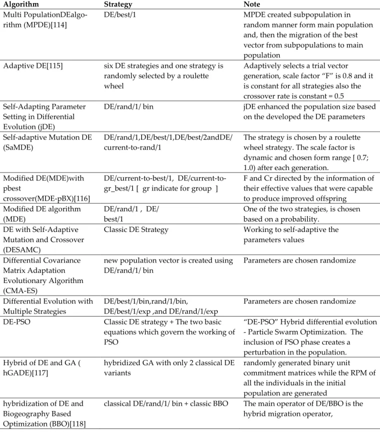
where g and G are the current generation number and the maximum number of generations, respectively. A few some remarkable DE algorithms are shortened in Table2.

(51)

51

Table 2.1.Summary of different DE algorithms with verity of approaches

Algorithm Strategy Note

Multi PopulationDEalgo-

rithm (MPDE)[114] DE/best/1 MPDE created subpopulation in random manner form main population and, then the migration of the best vector from subpopulations to main population

Adaptive DE[115] six DE strategies and one strategy is randomly selected by a roulette wheel

Adaptively selects a trial vector generation, scale factor “F” is 0.8 and it is constant for all strategies also the crossover rate is constant = 0.5 Self-Adapting Parameter

Setting in Differential Evolution (jDE)

DE/rand/1/ bin jDE enhanced the population size based on the developed the DE parameters Self-adaptive Mutation DE

(SaMDE) DE/rand/1,DE/best/1,DE/best/2andDE/ current-to-rand/1 The strategy is chosen by a roulette wheel strategy. The scale factor is dynamic and chosen form range [ 0.7; 1.0) after each generation.

Modified DE(MDE)with pbest

crossover(MDE-pBX)[116]

best/1,

DE/current-to-gr_best/1 [ gr indicate for group ] F and Cr directed by the information of their effective values that were capable to produce improved offspring

Modified DE algorithm

(MDE) DE/rand/1 , DE/ best/1 One of the two strategies, is chosen based on a probability. DE with Self-Adaptive

Mutation and Crossover (DESAMC)

Classic DE Strategy Working to self-adaptive the parameters values

Differential Covariance Matrix Adaptation Evolutionary Algorithm (CMA-ES)

new population vector is created using

DE/rand/1/ bin Parameters are chosen randomize Differential Evolution with

Multiple Strategies DE/best/1/bin,rand/1/bin, DE/best/1/exp ,and DE/rand/1/exp Parameters are chosen randomize DE-PSO Classic DE strategy + The two basic

equations which govern the working of PSO

“DE-PSO” Hybrid differential evolution - Particle Swarm Optimization. The inclusion of PSO phase creates a perturbation in the population. Hybrid of DE and GA (

hGADE)[117] hybridized GA with only 2 classical DE variants randomly generated binary unit commitment matrices while the RPM of all the individuals in the initial

population are generated hybridization of DE and

Biogeography Based Optimization (BBO)[118]

classical DE/rand/1/ bin + classic BBO The main operator of DE/BBO is the hybrid migration operator,

(52)

52

CHAPTER 3: RESEARCH PLAN

3.1 Introduction

The DE algorithm has been applied in several applications such as scheduling, image processing, multi-modal methods, non-convex methods, and among many others [119-121]. The traditional performance of DE is based on the chosen strategy and the control parameters[122, 123]. This strategy consists of mutation, crossover, and selection, and there are three control parameters: the number of populations “NP”, the mutation factor “F” (sometimes called the scaling factor), and the crossover rate “Cr”[124-126]. Indeed, the performance of DE relies on the values of the population size “NP”, the mutation factor “F”, and the crossover rate” Cr”[127, 128]. Many studies have been conducted in classic DE, such as using mutation with perturbation, mutation with selection pressure, and a neighborhood mutation operator[129].

The second phase is the crossover and there are two different crossover techniques, either binomially or exponentially, produced different quality of results[40, 130]. The major aspect of the crossover is to determine the element of the trail vector that will be inherited from the target vector[131]. Additionally, the performance of DE relies on strategies and the right control parameter values [132-135]. Extensive researches have been conducted to determine what the best control parameter values. There are two approaches for setting these control parameters: predefined (also called deterministic) and adaptive approaches. In fact, in the deterministic technique there are some recommended

(53)

53

values for these parameters for which it is not required to obtain any feedback. However, with adaptive technique the parameters values assigned and adjusted dynamically through the processing according to pre-defined rules. Unfortunately, the adaptive and self-adaptive techniques that are often time-consuming for the evolution for each parameter value because of their high complexity[136]. In fact, adaptive and self-adaptive are very effective for small dimensional problems, however they are produce poor results when the dimensions are increased[137]. Therefore, researchers have focused on finding suitable and efficient strategies to speed up the convergence rate[138, 139].

In this work we introduce a new proposes a Multi-Layer Strategies Differential Evolution (MLSDE) approach, which uses different mutation strategies in order to reach a fast convergence rate and avoid premature convergence due to the loss of diversity in the population. Multilayer techniques were applied since there is no single method that has proven fit for every problem. Some strategies may work perfectly with some problems, while other strategies perform poorly with other problems. ndeed the MLSDE works to improve the diversification of offspring by using different strategies in a multiple-layered approach. This approach spread out the population so that the sampled vectors can easily generate improved offspring. One of the advantages of this technique is its ability to reach a very quick rate of convergence to find the optimal solution with a minimum number of iterations.

(54)

54

3.2 Multi-Layer Strategies Differential Evolution

The multi-layer strategies differential evolution (MLSDE) approach operates in the same manner as classic differential evolution with an initialization population, mutation, crossover, and then the selection operation. However, MLSDE consists of a group of mutations, crossovers, and selections that are performed in sequence.

In MLSDE, the first step is to initialize the main matrix with random population within constraints of upper and lower bound values. Then, the different vectors are chosen as the core of the mutation operations. These vectors differ in the way in which they present in domain space because of their different composition. Therefore, to obtain the diversity of the domain space, six vectors are chosen V1, V2, V3, V4, Vbest, and VHill from the population. Two approaches are used to construct the best vectors. The first approach, Vbest uses the objective functions to find best vector in the main matrix, whereby each row represents an independent vector. The second approach, uses Hill Climb method to construct vector VHill. The best vectors would often leads to a fast convergence and performs well when solving for unimodal problems. The combination of Vbest, and VHill helps to balance between exploration and exploitation.

(55)

55

Following the mutation stage the, the crossover between vectors occurs to produce improved vectors [136]. Crossover results in high diversity in populations by applying the crossover equations (11),(12), and (13).The crossover probability, Cr ∈ [0,1], is pre-defined value that controls the fraction of parameter values that are copied from the mutant. To control which source contributes a given parameter, uniform crossover. Compares Cr to the output of a uniform random number generator ,randj(0,1). If the random number is less than or equal to Cr, the trial parameter is inherited from the mutant, Vi, j otherwise, the parameter is copied from the vector, Xi, j . In addition, the trial parameter with randomly chosen index, jrand, is taken from the mutant to ensure that the trial vector does not duplicate Xi, j Because of this additional demand, Cr only approximates the true probability that a trial parameter will be inherited from the mutant[140].

(56)

56

Once chosen, the different vectors are used in the below equations to calculate new vectors Vy1 , Vy2, and Vy3. This stage is referred to as the MLSDE mutation.

Next stage is selection stage. The trail vectors produced from equation (11),(12) and (13) are compared with target vectors. If the trial vector, U1(i,j), U2(i,j), and U3(i,j) have an equal or lower objective function value than that of its target vector, X1(i,j), X2(i,j) , and U3(i,j) they replace the target vector in the next generation; otherwise, the target retains its place in the population. The flowchart of MLSDE algorithm is prsented in Figure.2.

(57)

57

(58)

58

CHAPTER 4: IMPLEMENTATION AND RESULTS

4.1 Implementation and Test Plan

We have conducted experimental tests on the optimization benchmark suite four typical minimization problems introduced in the CEC 2013 benchmark functions suite experiments. Therefore, the growing research area is divided into adaptive, self-adaptive, and hybridization strategies. Thus, this study may provide a roadmap through which developers may gain a full understanding of this field. To evaluate the reliability and robustness of the different DE algorithms, we introduce a general framework that includes the control parameters for evaluating the efficiency of the different algorithms. In addition, the proposed MLSDE algorithm is examined on the classical benchmark functions provided by the CEC2015 Special Session.

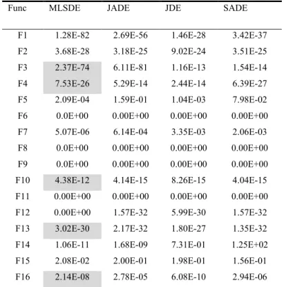
4.2 Results

The well-studied domain of function optimization was used to test the performance of the proposed MLSDE algorithm , which was evaluated based on the classical benchmark functions provided by the CEC2015 Special Session [141]. The algorithms was used for the comparison of different algorithms include JADE, JDE, and SADE [141, 142]. In this section, MLSDE is employed to minimize a set of 16 scalable