WIND TUNNEL TESTING: A GENERAL OUTLINE

(1)

Alan G. Davenport Wind Engineering Group

The Boundary Layer Wind Tunnel Laboratory

WIND TUNNEL TESTING:

A GENERAL OUTLINE

May 2007

The University of Western Ontario, Faculty of Engineering Science

London, Ontario, Canada N6A 5B9; Tel: (519) 661-3338; Fax: (519) 661-3339 Internet: www.blwtl.uwo.ca; E-mail: [email protected]

(2)

WIND TUNNEL TESTING: - i - Alan G. Davenport Wind Engineering Group A GENERAL OUTLINE

5 THE PEDESTRIAN LEVEL WIND SPEED TEST 8

6 THE TESTING OF LONG SPAN BRIDGES 9

7 OTHER TESTS 10

REFERENCES 11

APPENDIX A A-1

THE DEFINITION OF WIND CLIMATE A-1

A.1 Introduction A-1

A.2 Natural Wind A-1

A.3 Availability of Wind Records A-2

A.4 Probability Distribution of Mean Wind Speed and Direction A-3 A.5 Applicability of the Wind Climate Model A-4

APPENDIX B B-1

THE DEFINITION OF A HURRICANE WIND CLIMATE B-1

B.1 Introduction B-1

B.2 The Approach Used B-1

B.3 Verifying the Approach B-2

B.4 The Wind Climate for a Particular Site B-2

APPENDIX C C-1

THE MEASUREMENT AND PREDICTION OF SURFACE PRESSURE C-1

C.1 Experimental Technique C-1

C.2 Experimental Time Scale C-1

C.3 Choice of Sampling Period C-2

(3)

WIND TUNNEL TESTING: - ii - Alan G. Davenport Wind Engineering Group A GENERAL OUTLINE

C.5 General Characteristics of the Pressure Response C-3 C.6 Predictions of Peak Pressures and Suctions C-3 C.7 Limitations on the Predicted Peak Pressures and Suctions C-3

APPENDIX D D-1

PREDICTING PEAK RESPONSES FOR VARIOUS RETURN PERIODS D-1

D.1 Introduction D-1

D.2 The Prediction Process D-1

D.3 The Rate of Up-crossing of Peak (Maximum or Minimum) Response Values D-2

APPENDIX E E-1

STORM PASSAGE PREDICTIONS OF WIND LOADS AND RESPONSES E-1

E.1 Overview E-1

E.2 Extreme-value Predictions from Time-domain Analysis E-1 E.3 Examples of Predictions of Wind Loads and Effects E-2

E.4 Wind Directionality E-3

APPENDIX F F-1

DETERMINATION OF INTERNAL PRESSURE COEFFICIENTS AND THE FORMATION OF

DIFFERENTIAL PRESSURE COEFFICIENTS F-1

F.1 Summary F-1

F.2 Introduction F-1

F.3 Mean Internal Pressures: Distributed Leakage F-1 F.4 Mean Internal Pressures: Large Openings F-2

F.5 Fluctuating Internal Pressures F-3

F.6 Forming Differential Pressure Coefficients at BLWTL F-4 F.7 Limitations of Predicted Differential Pressures F-5

APPENDIX G G-1

DETERMINATION OF TOTAL DYNAMIC LOADS USING A RIGID MODEL/FORCE BALANCE

TECHNIQUE G-1

G.1 Summary G-1

G.2 Introduction G-1

G.3 Concepts of the Force Method G-1

G.4 Concept of the Balance G-2

G.5 Linear Elastic Response Calculations with the BLWT Balance G-2

G.6 Torsional Response G-4

APPENDIX H H-1

AEROELASTIC SIMULATIONS OF BUILDINGS USING TWO-DEGREE-OF-FREEDOM MODELS H-1

H.1 Introduction H-1

H.2 Aeroelastic Modelling H-1

H.3 Details of the Aeroelastic Model H-2

H.4 Experimental Procedure and Preliminaries H-2 H.5 Predictions of Peak Wind-Induced Response H-3

APPENDIX I I-1

AEROELASTIC SIMULATIONS OF BUILDINGS USING MULTI-DEGREE-OF-FREEDOM MODELS I-1

I.1 Introduction I-1

(4)

WIND TUNNEL TESTING: - iii - Alan G. Davenport Wind Engineering Group A GENERAL OUTLINE

I.3 Details of the Aeroelastic Model I-2

I.4 Experimental Procedure and Preliminaries I-2 I.5 Predictions of Peak Wind-induced Response I-3

APPENDIX J J-1

DETERMINATION OF TOTAL DYNAMIC LOADS FROM THE INTEGRATION OF SIMULTANEOUSLY MEASURED PRESSURES J-1

J.1 Summary J-1

J.2 The Integration Procedure J-1

J.3 Response Calculations J-1

APPENDIX K K-1

THE EVALUATION AND USE OF EFFECTIVESTATIC FORCE DISTRIBUTIONS K-1

K.1 Effective Static Force Distributions K-1

K.2 Combined Load Cases K-2

APPENDIX L L-1

THE PEDESTRIAN LEVEL WIND ENVIRONMENT L-1

L.1 Introduction L-1

L.2 Test Procedure L-1

L.3 Statistical Predictions of Pedestrian Level Winds L-1 L.4 Acceptance and Safety Criteria for Pedestrian Level Wind Conditions L-2

APPENDIX M M-1

DYNAMIC WIND FORCES ON LONG SPAN BRIDGES USING EQUIVALENT STATIC LOADS M-1

M.1 Introduction M-1

M.2 The Description of Design Loads M-1

M.3 Evaluation of the Modal Load W1 and W2 M-1 M.4 Experimental Determination of Design Load Components M-4

M.5 Determination of Design Wind Loads M-4

(5)

WIND TUNNEL TESTING: - iv - Alan G. Davenport Wind Engineering Group A GENERAL OUTLINE

LIST OF TABLES

TABLE L.1 CRITERIA FOR PEDESTRIAN COMFORT AND SAFETY...L-3 TABLE L.2 EXTRACTS FROM THE BEAUFORT SCALE ...L-4

(6)

WIND TUNNEL TESTING: - v - Alan G. Davenport Wind Engineering Group A GENERAL OUTLINE

LIST OF FIGURES

FIGURE B.1 COMPARISON OF TYPHOON WIND SPEEDS AT WAGLAN ISLAND TO

MEASURED DATA CORRECTED FOR TOPOGRAPHIC EFFECTS ... B-5 FIGURE B.2 PREDICTED PEAK ACCELERATIONS FOR THE ALLIED BANK DURING

HURRICANE ALICIA... B-6 FIGURE D.1 ILLUSTRATION OF THE PREDICTION PROCESS ... D-4 FIGURE E.1 OBSERVED 10-MINUTE AVERAGE SURFACE WIND SPEED AND WIND

DIRECTION AT HONG KONG DURING TYPHOON YORK (SEPTEMBER 16,

1999). ... E-5 FIGURE E.2 TYPICAL WIND INDUCED RESPONSE SHAPES... E-5 FIGURE E.3 COMPARISON OF GENERIC WIND LOADS AND EFFECTS PREDICTED

FOR DIFFERENT WIND DIRECTIONS USING CONVENTIONAL

STATISTICAL METHODS AND TRACKING THE EFFECTS OF INDIVIDUAL

STORMS... E-6 FIGURE E.4 COMPARISON OF PEAK STRUCTURAL WIND LOAD EFFECTS FOR

BUILDINGS A AND B HYPOTHETICALLY LOCATED IN DIFFERENT WIND REGIONS PREDICTED BY CONVENTIONAL STATISTICAL METHODS AND

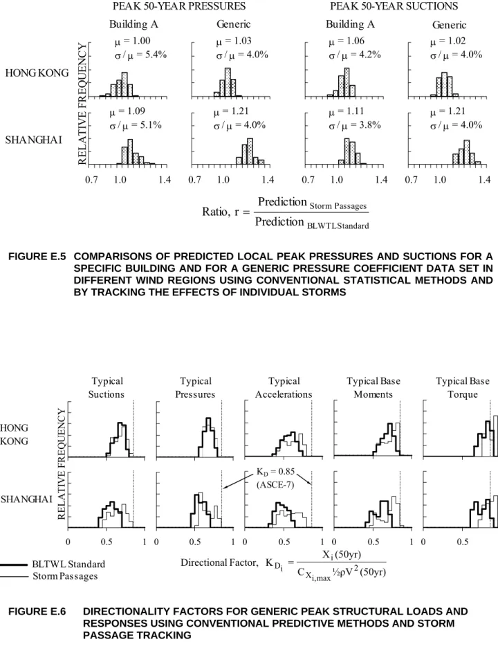
BY TRACKING THE EFFECTS OF INDIVIDUAL STORMS ... E-6 FIGURE E.5 COMPARISONS OF PREDICTED LOCAL PEAK PRESSURES AND

SUCTIONS FOR A SPECIFIC BUILDING AND FOR A GENERIC PRESSURE COEFFICIENT DATA SET IN DIFFERENT WIND REGIONS USING

CONVENTIONAL STATISTICAL METHODS AND BY TRACKING THE

EFFECTS OF INDIVIDUAL STORMS... E-7 FIGURE E.6 DIRECTIONALITY FACTORS FOR GENERIC PEAK STRUCTURAL LOADS

AND RESPONSES USING CONVENTIONAL PREDICTIVE METHODS AND

STORM PASSAGE TRACKING ... E-7 FIGURE G.1 DYNAMIC RESPONSE OF THE BALANCE-MODEL COMBINATION ... G-6 FIGURE H.1 SCHEMATIC OF THE AEROELASTIC MODEL ... H-4 FIGURE I.1 SCHEMATIC OF THE AEROELASTIC MODEL ...I-4 FIGURE M.1 DISTRIBUTED WIND LOAD COMPONENTS ...M-6 FIGURE M.2 NOTATION ...M-6 FIGURE M.3 SPECTRUM OF MODAL LOAD AMPLITUDE ...M-7 FIGURE M.4 SUNSHINE SKYWAY BRIDGE...M-7 FIGURE M.5 SECTION MODEL RESPONSE (UNCORRECTED) ...M-8 FIGURE M.6 VERTICAL VELOCITY SPECTRUM...M-9 FIGURE M.7 AERODYNAMIC ADMITTANCE RESPONSE (UNCORRECTED) ...M-9

(7)

WIND TUNNEL TESTING: - vi - Alan G. Davenport Wind Engineering Group A GENERAL OUTLINE

FIGURE M.8 JOINT ACCEPTANCE FUNCTION...M-10 FIGURE M.9 DAMPING FUNCTIONS ...M-10 FIGURE M.10 WIND LOAD COMPONENTS ON COMPLETED BRIDGE ...M-11

(8)

WIND TUNNEL TESTING: - 1 - Alan G. Davenport Wind Engineering Group A GENERAL OUTLINE

1 INTRODUCTION

This document provides a general outline of common wind tunnel tests performed at the Boundary Layer Wind Tunnel Laboratory (BLWTL) at the University of Western Ontario. It also details some of the techniques used to analyse the data from these tests. Since it is a general outline, it will cover some tests and analyses not performed for a particular project. Other than the wind climate modelling discussed in Section 2 and Appendices A and B, and the prediction methodology discussed in Appendices D and E, the various tests and analysis methodology are independent and the reader may skip sections that are not relevant. Also, this report does not, by any means, attempt to cover all of the types of tests and analyses performed at the Laboratory. Unusual tests are covered in separate reports for the projects employing them.

In determining the effects of wind for a particular development, there are two main ingredients to consider. The first comprises the aerodynamic characteristics of the development. These are simply the effects of the wind when it blows from various directions. This information only has limited value, however, without knowing how likely it is that the wind will blow from those directions and how strongly it is likely to blow. This climatological information, in the form of a probability distribution of wind speed and direction, is the second main ingredient needed for determining wind effects for a particular development. The aerodynamic information is characteristic of the particular development and its immediate surroundings, while the wind climate information is characteristic of the geographical location of the development. Both are necessary to determine the wind effects for a particular development and, when combined, provide statistical predictions of the wind effects which are independent of wind direction.

At the BLWTL, the aerodynamic characteristics of the development are commonly determined through model studies of the project. These studies may include measurements of various types of information of interest, such as cladding loads, structural loads and pedestrian level wind speeds, as detailed in the following sections of this report. The probability distribution of wind speed and direction, is determined from analyses of historical wind speed and direction records taken near the site of the development. Details of these analyses are included in Appendix A. Tropical cyclones, such as hurricane or typhoon winds present a special case and their associated statistical characteristics are handled separately using different analysis methods. These are detailed in Appendix B.

In all cases, tests carried out at the BLWTL are in accordance with the state-of-the-art, and meet or exceed such test requirements as documented by the ASCE Manual of Practice (1).

(9)

2 THE MODELLING OF THE SITE AND THE WIND

2.1 General

The basic tool used is the Laboratory's Boundary Layer Wind Tunnel. This wind tunnel is designed with a very long test section, which allows extended models of upwind terrain to be placed in front of the model of the development under test. The modelling is done in more detail close to the site. The wind tunnel flow then develops characteristics which are similar to the wind over the terrain approaching the actual site. This methodology has been highly developed and further details can be found in References 2, 3 and 4.

The modelling is comprised of the following components:

1. A detailed model of the development. Different types of model are used for the various types of test. These are discussed below in the sections on the individual tests.

2. A detailed proximity model of the surrounding area, built in block outline from wood and Styrofoam. Depending on the scale and size of the model, this may extend for a radius of approximately 500 to 600 metres.

3. Coarsely modelled upstream terrains, chosen to represent the general roughness upstream of the site for particular wind directions. Typically, several models are chosen, each used for a range of wind directions.

For project sites close to hilly terrain or with unusual topography, topographic study may be carried out to establish the wind characteristics at the site. This may be in the form of topographic model study at a small scale (~1:3000) or computational methods. The resulting target wind characteristics will be modelled in the larger scale used in the building or bridge tests.

2.2 Scaling

The fundamental concept is that the model of the structure and of the wind should be at approximately the same scale. The natural scaling of the flow in the wind tunnel is in the range 1:400 to 1:600; however, in some cases, instrumentation or other requirements may demand a larger model. In these cases, additional flow modification devices may be used to approximate larger scale flows.

In all cases, it is the mean wind speed profile and the turbulence characteristics over the structure that are most important to match with those expected in full scale. Guidance as to the latter is obtained through direct full scale measurements as compiled by ESDU (5, 6). Such data are also used to ensure that the test speeds near the top of the building are properly interfaced with full scale wind speeds predicted to occur at the full scale site.

(10)

3 THE CLADDING LOADS TESTS

3.1 Pressures

and

Suctions on Exterior Surfaces

Detailed measurements of the pressures and suctions on exterior surfaces of the building or structure are made using a rigid model that accurately represents the detailed exterior geometry of the development. The model contains numerous (typically 300 to 800) holes or "taps" which are connected via tubing to pressure transducers. The transducers convert the pressure at the point where the tap is located to an electrical signal which is then measured by the Laboratory's computerized data acquisition system. The technology employed allows all pressures on the building to be measured essentially simultaneously for a particular wind direction. Measurements are usually made at 10° intervals for the full 360° azimuth range. A detailed description of the procedures followed and the definitions used are presented in Appendix C.

These aerodynamic measurements made in the wind tunnel are subsequently combined with the statistics of the full scale wind climate at the site using the methodology outlined in Appendices D and E to provide predictions of pressures and suctions for various return periods.

3.2 Scaling

The aerodynamic pressure coefficients can be converted to full scale pressure values based on consistent length, time and velocity scaling between full scale and model scale. This applies very well for sharp-edged structures. For structures with curved surfaces, additional care has to be taken to ensure that the flow regime is consistent in model and full scale, as well as in the interpretation of the results.

For typical building tests, length scale is in the order of 1:300 to 1:500. Velocity scale is approximately 1:3 to 1:5. Time scale is in the order of 1:100. For example, 36 seconds in model scale represents about an hour in full scale and the data will be taken about 100 faster in the test than in full scale. Further details regarding scaling can be found in Appendix C.

3.3 Internal Pressures and Differential Pressures

The net load on cladding is the difference between the external and internal pressures. Using the methodology described in Appendix F, mean internal pressures are determined at all wind angles. These are then subtracted from the appropriate external pressure coefficients to form differential pressure coefficients. Finally, the coefficients are combined with the statistics of the full scale wind climate at the site, using the methodology outlined in Appendices D and E, to provide predictions of differential pressures and suctions for various return periods.

In the case of large opening due to operable windows or breach of the building envelope, large internal pressures may develop. Typically, the external pressure at the opening will be transmitted into the building interior volume. Building envelope at other locations within the building volume will experience both the external pressures at those external locations as well as the large internal pressure transmitted from the opening.

For free standing elements with both sides exposed to air, such as parapets and canopies, the net differential pressures are the instantaneous difference in pressures on the opposite sides.

(11)

4 THE DETERMINATION OF OVERALL STRUCTURAL LOADS AND

RESPONSES

4.1 Introduction

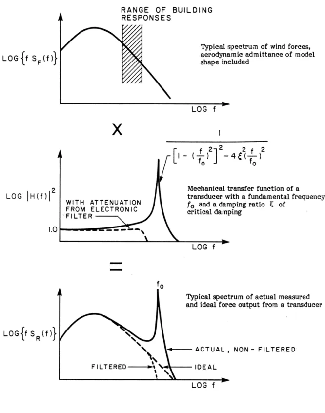
The dynamic response of most tall buildings to wind is primarily the results of building motions in the fundamental sway and torsion modes of vibration with relatively small contributions from higher modes. The mechanical transfer function, relating the load function to the response, is straightforward. On the other hand, the aerodynamic transfer function, relating the gust structure to the wind induced forces is difficult to establish without wind tunnel model tests. A further complication exists if body motion effects interact with the load function (aerodynamic damping).

Multi-degree-of-freedom aeroelastic models have traditionally been used to study the action of wind on sensitive buildings and structures. While such simulations provide the most direct and reliable estimates, the required models are expensive and time consuming to design and construct. Two-degree-of-freedom aeroelastic models, which simulate the wind induced responses in the two fundamental sway modes of vibration, while less expensive, do not provide information on torsion effects, which may be significant for buildings of unusual shape and structural dynamic properties. In both of these cases, the model moves in the wind tunnel just as it would in full scale; its response in the wind tunnel can be scaled directly to full scale.

A high-frequency balance/model system can measure the load function directly, provided that aerodynamic damping effects are negligible, which is usual for most buildings at practical wind speeds and practical structural damping values. (Note that if such effects are important, they can be accounted for by using a supplemental testing technique in which the model is oscillated). The now commonly used high frequency force balance technique was originally developed at the BLWTL.

One other method for determining the load function is to integrate the point pressure measurements on an instant-by-instant basis to form time histories of the generalized forces.

4.2 The Force Balance Test

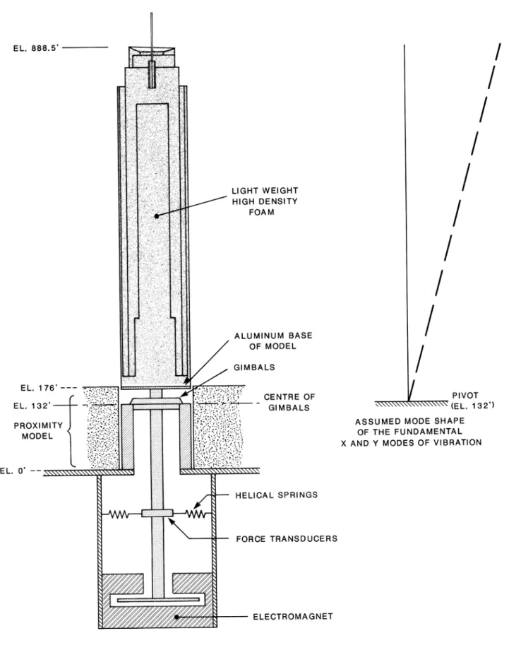
This technique involves testing a lightweight, stiff, geometrical representation of the building on an ultra-sensitive force balance. The technique allows direct measurements of good approximations to the steady and unsteady modal forces acting in the fundamental sway and torsional modes of vibration of the building. The dynamic responses including resonant amplification at the natural frequencies of the building are derived analytically for each mode using random vibration analysis methods and are subsequently used to provide estimates of the full scale responses of the building. As a result, this method is very accommodating of changes to the structural properties after testing, since the analytical procedure can be simply repeated using the same experimental results, which remain applicable so long as the aerodynamic characteristics of the building remains the same. A detailed description of this method is presented in Appendix G.

Time histories of the base shears and moments are taken during the tests. From these, the mean and rms (root-mean-square) base bending moments along orthogonal building axes, as well as mean and rms base torque are determined. The base bending moments represent a good approximation to the generalized modal forces in the fundamental modes. The spectra of the generalized modal forces are also determined from these time histories and used to determine the resonant component of the response. Measurements are usually taken at 10° intervals for the full 360° azimuth range.

Scaling is essentially the same as for pressure tests, requiring scaling of the structure to the flow model only, with the non-dimensionalized data being independent of test speed; however, in this case, the time scaling must be chosen carefully to ensure that the prototype’s natural periods of interest fall within the accurate measuring range of the model/balance combination.

(12)

Once the responses have been determined, they are combined with the statistics of the full scale wind climate at the site, using the methodology outlined in Appendix D, to provide predictions of loads and responses for various return periods.

4.3 The Two-degree-of-freedom Aeroelastic Test

This technique requires scaling the dynamic properties (mass, stiffness and period) of the building in the fundamental sway modes and measuring the response to wind loads directly. The building is modelled as a rigid body, pivoted near the base, with the elasticity provided by appropriately selected springs. Implicit in this technique is the assumption that the sway modes do not include any coupling and can be approximated as linear, and that torsion is unimportant. These prove to be reasonable assumptions for a large range of buildings. A full discussion of this technique is contained in Appendix H.

The advantage of this technique is that the measurements will include effects of aerodynamic damping that are not included when using the force balance technique. It is also a simpler, less expensive technique than a multi-degree-of-freedom aeroelastic test. The disadvantages of the technique are that it is limited by the assumptions noted above and it is more complicated and expensive than the force balance technique while being less accommodating of changes to the dynamic properties of the building after the test. Furthermore, its advantage over the force balance technique, namely the inclusion of aerodynamic damping effects, rarely proves to be necessary since the aerodynamic damping is usually small and positive (i.e. it reinforces the inherent structural damping), but can be negative if vortex shedding plays an important role in the dynamic response. For most buildings, vortex shedding occurs at speeds well above the range of speeds that the structure will be subjected to. Nevertheless, it is useful for confirming force balance results and confirming that aerodynamic damping effects are indeed negligible.

As with other types of tests, once the aerodynamic data has been measured for a full range of wind directions, it is combined with the statistics of the full scale wind climate at the site, using the methodology outlined in Appendix D, to provide predictions of loads and responses for various return periods.

4.4 The Multi-degree-of-freedom Aeroelastic Test

This technique requires scaling the dynamic properties (mass, stiffness, periods and mode shapes) of the building in the fundamental sway modes and the fundamental torsion mode, including any coupling within modes. Some higher modes of vibration are also modelled. The responses to wind loads are then measured directly. Typically, a building is modelled as a series of lumped masses joined by appropriately sized columns; for towers, other approaches to produce the elastic model can also be used. A full discussion of this technique is contained in Appendix I.

The advantage of this technique is that the measurements will include effects of aerodynamic damping, vortex shedding, coupling within modes and some higher modes that are not fully dealt with when using the force balance technique. For most buildings, however, it can be argued that the aerodynamic damping effects are likely to be small, higher modes can be neglected and that the force balance adequately handles coupled modes analytically. Nevertheless, for more complicated structures, the additional reassurance of an aeroelastic test may be justified.

The disadvantages of the technique are that the model is time consuming and expensive to build. The model is also designed for a single set of building dynamic properties and approximations must be made if these change. The force balance technique on the other hand, yields results equally applicable to any set of building dynamic properties.

As with other types of tests, once the aerodynamic data has been measured for a full range of wind directions, it is combined with the statistics of the full scale wind climate at the site, using the methodology outlined in Appendix D, to provide predictions of loads and responses for various return periods.

(13)

4.5 Overall Loads from Local Pressure Measurements

The development of solid state pressure scanners, which permit the simultaneous measurement of pressures at many points on the surface of a building, allows the determination of instantaneous overall wind forces from the local pressure measurements. The technique allows direct computation of the steady and unsteady modal forces acting in any number of modes of vibration of the building. In similar fashion to the force balance approach, the resonant amplification due to the building's structural dynamics is derived analytically for each mode using random vibration analysis methods and results are subsequently used to provide estimates of the full scale response of the building. A detailed description of this method is presented in Appendix J. (Note that integration can also yield true time histories of loads on building subcomponents of interest, such as canopies, large panels, or roofs).

The advantages of this technique are that a single model used in a single testing session can produce both overall structural loads and cladding loads. The testing parameters would be extended to ensure that the local pressure data taken is also sufficient for the analysis of structural loads. The analysis required to determine structural loads from the local pressure information is nominally the same as that from the force balance tests. This technique also has the advantage of properly determining the generalized forces for three-dimensional non-linear mode shapes. Although these are also properly handled in multi-degree-of-freedom aeroelastic tests through the proper design of the aeroelastic model, such tests are expensive and time-consuming. The force balance technique can handle three-dimensional mode shapes but need to have corrections for non-linear modes. The pressure integration technique can also be used to examine higher modes with non-monotonic mode shapes.

A disadvantage of this technique is that the cladding pressure test model typically includes more instrumentation and takes longer to construct than a force balance test model. Also, as in the force balance technique, it does not include any effects of the building's motion through the air, such as aerodynamic damping; however, neglecting these effects is usually slightly conservative. Proper integration of local pressures to obtain overall wind forces requires that all buildings surfaces are properly represented in the model instrumentation and subsequent calculations. This may not be possible for buildings or structures with complex geometry or small components.

Once the responses have been determined, they are combined with the statistics of the full scale wind climate at the site, using the methodology outlined in Appendix D, to provide predictions of loads and responses for various return periods.

4.6 Effective

Static Force Distribution

Representative effective static force distributions reflecting the combined static and dynamic response of the building are evaluated for the x, y and torque directions. The details of the procedure are included as Appendix K.

In principle, for any azimuth, effective static force distributions can be determined which reproduce the measured dynamic peak base bending moment. The particular vertical distribution chosen must reflect the actual static and dynamic loading of the building.

The loading is reasonably considered to be made up of the mean loading, the dynamic loading due to background or quasi-steady excitation and the dynamic inertial loading due to resonant oscillations. The mean loading distribution is determined from the integration of mean external local pressures from the cladding loads test or from an assumed distribution chosen to reflect the mean wind speed distribution. The inertial dynamic loading distribution is determined from the known vibration properties of the building. The measurement of the relative contribution of the unsteady and steady components at the base from one of the above structural loads tests is used to combine the mean and dynamic distributions into one total distribution. An overall effective loading diagram, independent of wind direction, is then constructed by averaging the effective force distributions, weighted by the relative importance of each wind direction.

It should be appreciated that these effective static loading distributions are representative of the most likely severe wind loading conditions expected, but the detailed loading may change somewhat for

(14)

different wind directions, since both the details of the mean pressure distribution and the mix between mean and resonant response will alter from angle to angle. Nevertheless, they provide useful distributions of loading for the design of the structural members in the overall wind resisting system.

4.7 Load Combination Factors

The determination of the wind-induced loads as described above treats the load directions independently. It should be recognized that wind loads in all three principal directions will occur simultaneously although the peak loads in each respective directions will not all occur at the same time. Load combination factors are used to specify the required simultaneous application of loads in the three directions such that the major load effects are reproduced for design purposes. These can be in the form of general load reduction factors applied to all three load directions or companion load factors where the full application of the load in the main load direction is accompanied by reduced loads in the other load directions.

Appendix K describes the companion load method used at the BLWTL. This method is based on the assumed critical load effects using generic influence factors due to base moments. While this is applicable to buildings or other like-line structures, other spatial structures such as canopies or load building frames may have different critical load effects and require other analytical procedures such as the LRC (Load-Response-Correlation) method to determine the effective load shapes and load combination factors.

(15)

5 THE PEDESTRIAN LEVEL WIND SPEED TEST

This test is usually performed using the same model that was used for the cladding loads test, and may include some landscaping details. The model is instrumented with omni-directional wind speed sensors at various locations around the development where measurements of the mean and fluctuating wind speed are made for a full range of wind angles, usually at 10° intervals.

The scaling involved is the same as that of the modelled wind flow. Thus, the ratio of a wind speed near the ground to a reference wind speed near the top of the building is assumed to be the same in model and full scale, and to be invariant with both test speed and prototype speed. Since the thermal effects in the full scale wind are neglected, strictly speaking, the results are only applicable to neutrally-stable flows which are usually associated with stronger wind speeds. However, near tall buildings, local acceleration effects due to the local geometry are usually dominant over thermal effects, and are also the most important for design considerations.

The measured aerodynamic data is combined with the statistics of the full scale wind climate at the site, using the methodology outlined in Appendix D, to provide predictions of wind speeds at the site. Two types of predictions are typically provided:

1. Wind speeds exceeded for various percentages of the time on an annual basis. Wind speeds exceeded 5% of the time can be compared to comfort criteria for various levels of activity. Very roughly, this is equivalent to a storm event of several hours duration occurring about once per week.

2. Predictions of wind speeds exceeded during events or storms with different frequencies of occurrence. Wind speeds exceeded once per year can be compared to criteria for pedestrian safety.

A more detailed description of this type of test is presented in Appendix L.

Other, non-quantitative techniques are also available to determine levels of windiness over a project site. One of these techniques is a scour technique in which a granular material is spread uniformly over the area of interest. The wind speed is then slowly increased in increments. The areas where the granular material is scoured away first are the windiest areas, while areas that are scoured later as the wind speed increases represent progressively less windy areas. Photographs of the scour patterns at increasing wind speeds can be superimposed using image processing technology to develop contour diagrams of windiness. This information can be used to determine locations for quantitative measurements, or simply to identify problem areas where remedial measures are necessary. Testing several configurations can provide comparative information for use in evaluating the effects of various architectural or landscaping details. The advantage of the scour technique is that it can provide continuous information on windiness over a broad area, as opposed to the quantitative techniques which provide wind speeds at discrete points.

An even more qualitative technique is to introduce smoke to visualize flow paths and accelerations at arbitrary places. This can be a useful exploratory technique by which to understand the flow mechanisms and how best to alter them.

(16)

6 THE TESTING OF LONG SPAN BRIDGES

The definition of wind effects on long span bridges should include not only the identification of any aerodynamic instability, but also the loading under turbulent flow conditions representative of full scale conditions. Recognition of the importance of lift and torsional loading in addition to drag loading is also essential. Thus the study of wind effects on a bridge includes some or all of the following:

1. Selection of a bridge deck system with favourable aerodynamic characteristics. There is a reasonably broad range of bridge cross-sections which have been tested, the results of which can be used as guidance in the design of new bridges.

2. Measurement and definition of the response and aerodynamic characteristics of the bridge deck. This is accomplished by testing the selected bridge cross-section using an elastically mounted section model and/or a "taut strip" model. These tests indicate any tendency to instability and the speeds at which this may occur. As well, the aerodynamic loads measured can be combined with statistics of the full scale wind climate at the site using the methodology outlined in appendix D to provide predictions of responses for various return periods. A full description of the determination of dynamic wind forces using equivalent static loads is given in Appendix M. 3. Confirmation of bridge behaviour using a multi-degree-of-freedom aeroelastic model of the entire

bridge. This would be recommended in cases of innovative design and bridges of exceptional size and importance or unusual siting. The methodology for this test is similar to that for tall buildings, as described in Appendix I. Aeroelastic bridge models can also be used to determine general design load information for the bridge, and is especially useful for multi-span bridges whose spans are slightly different in dynamic properties.

4. Special Aspects. These may include the definition of loads during construction, cable movements, tower loads, fatigue and the role of damping.

(17)

7 OTHER TESTS

As mentioned in the introduction, this report is intended to give some background information on common tests performed at the BLWTL. There are many other, less common tests performed and new techniques are constantly being developed. Some of the techniques and tests available at the BLWTL are:

• dispersion of gaseous and particulate pollutants

• drifting and deposition of ice and snow

• monitoring of wind effects on full-scale structures

• influence of wind on heating, ventilation and air conditioning

• wind/wave effects on offshore structures

• wind induced iceberg drift

• influence of large-scale topography on wind patterns

• dynamics of inflated structures and tents

• evaluation of natural ventilation

• fatigue analysis

• galloping of cables and transmission lines

• interaction of multiple structures, both structurally independent and linked

• dynamics of foundations

• seismic loading

• design of additional dampers for buildings, chimneys and cables

• cooling and evaporative effects of wind

• performance of wind generators and their siting

• cross-winds on ground vehicles

• influence of wind breaks on forestry and agriculture

• soil erosion

• drift and deposition of sprays

• wind effects on ponds, used for such purposes as aquiculture or protecting mine tailings from erosion

The activities of the Laboratory are by no means limited to the items above; research is under way in many areas related to wind, waves, dynamics and earthquakes. New challenges are always welcome.

(18)

REFERENCES

(1) American Society of Civil Engineers (ASCE). “Manual of Practice for Wind Tunnel Testing of Buildings and Structures”. 1999.

(2) Davenport, A.G. and Isyumov, N. "The Application of the Boundary Layer Wind Tunnel to the Prediction of Wind Loading", International Research Seminar on Wind Effects on Buildings and Structures, Ottawa, Canada, September 1967, University of Toronto Press, 1968.

(3) Surry, D. and Isyumov, N. "Model Studies of Wind Effects - A Perspective on the Problems of Experimental Technique and Instrumentation", Int. Congress on Instrumentation in Aerospace Simulation Facilities, 1975 Record, pp. 76-90.

(4) Whitbread, R.E., "Model Simulation of Wind Effects on Structures", NPL International Conference on Wind Effects on Buildings and Structures, Teddington, England, 1963.

(5) Engineering Sciences Data Unit (ESDU). “Strong Winds In The Atmospheric Boundary Layer. Part 1: Mean-Hourly Wind Speeds”, ESDU 82026, 1982.

(6) Engineering Sciences Data Unit (ESDU). “Strong Winds In The Atmospheric Boundary Layer. Part 2: Discrete Gust Speeds”, ESDU 83045, 1983.

(19)

WIND TUNNEL TESTING: - A-1 - Alan G. Davenport Wind Engineering Group A GENERAL OUTLINE

APPENDIX A

THE DEFINITION OF WIND CLIMATE

A.1 Introduction

The wind tunnel testing provides information regarding the dependence of particular response parameters on wind speed and direction. In order to make the most rational use of this aerodynamic information, it is necessary to synthesize it with the actual wind climate characteristics at the site. The characteristics necessary to define are those governing wind speed and direction at a suitable height above ground level at the site. The joint probability distribution of wind speed and direction then defines the wind climate, whereas all of the aerodynamic information, which includes sensitivities to building orientation and to its surroundings, is contained in the wind tunnel data.

A.2 Natural

Wind

Air flowing over the earth's surface is slowed down and made turbulent by the roughness of the surface. As the distance from the surface increases, these friction effects are felt less and less until a height is reached where the influence of the surface roughness is negligible. This height is referred to as the gradient height, and the layer of air below this, where the wind is turbulent and its speed slowly increases with height, is referred to as the boundary layer. During periods of neutral atmospheric stability, typical of strong wind conditions, the gradient height or depth of the earth's boundary layer is determined largely by the terrain roughness and typically varies from 270m over open country to about 500m over built-up urban areas (A-1, A-2).

In more technical terms, for slowly-moving pressure systems, the motion of air at heights above the influence of the earth's surface is essentially parallel to the isobars and is governed by the pressure gradient, the Coriolis acceleration and the centrifugal acceleration due to isobar curvature (A-3). If conditions are such that these three effects are in balance, it is referred to as gradient wind, and as the geostrophic wind if there is no isobar curvature. The height at which this balance is first approximately achieved, that is, the height where frictional effects due to the earth's surface cease to be significant, is termed gradient height. As used here, the term gradient wind refers to the measured wind at approximately 500m. This usage is not in exact agreement with the above definition but does provide a convenient terminology.

Within the atmospheric boundary layer the flow becomes increasingly more dependent on shear stresses of mechanical and buoyant origin. The mean wind speed within the atmospheric boundary layer increases markedly with height above ground and the orientation of the mean wind speed vector rotates somewhat with respect to its direction near the surface. This horizontal rotation or veering with height is clockwise in the northern hemisphere. Based on theoretical arguments, the resulting relationship between the surface and gradient mean wind speed and direction during neutrally-stable atmospheric conditions depends on the Rossby number which relates shear forces to forces from the Coriolis acceleration (A-1). However, Davenport (A-2) and others (A-4) have shown that the ratio of the surface-to-gradient wind speed is relatively insensitive to both the latitude and the gradient wind speed and depends primarily on the upstream terrain roughness. Furthermore, estimates of the angular shift between surface and gradient height for open terrain, typical of most anemometer locations, is generally of the order of the angular resolution of the measured wind direction, making it unnecessary to correct for this rotation for most wind engineering applications. Consequently, natural wind over a particular terrain can be simulated by a turbulent boundary layer flow developed in a wind tunnel over a long fetch of appropriate model terrain roughness. Details of this approach, which leads to a representative simulation of the mean flow structure and the turbulent flow characteristics are given elsewhere (A-5).

(20)

Two models are commonly used to describe the wind characteristics within the boundary layer. The power law profile gives the variation of the mean speed with height:

( )

m g g z z V z V _⎟⎟ ⎠ ⎞ ⎜ ⎜ ⎝ ⎛ = (A.1)

where V

( )

z is the mean wind speed at height z; is the gradient wind speed for the same azimuth; and and are the gradient height and the power law exponent respectively. In general both and

depend on the wind direction. This model is convenient and is used in most building codes.

g

V

g

z m z_g

m

The other model is based on the Harris and Deaves model described in the ESDU documents (A-6, A-7) which include the mean wind speed and turbulence characteristics.

Examining the power spectrum of all wind speed variations (the power spectrum indicates the distribution of energy with frequency), a distinct gap is found to exist at periods of about one hour (1, A-8, A-9). This spectral gap conveniently separates atmospheric motion into two distinct categories:

1. turbulent, with locally-stationary statistical properties

2. quasi-steady mean speeds associated with slowly-varying synoptic or climatological time scales. For wind tunnel simulations, the first is modelled by the wind tunnel flow itself, which reproduces the turbulence characteristics of the natural wind. The second is taken into account by the wind climate model developed for the site, based on historical climatological records.

A.3

Availability of Wind Records

Wind records, in the form of relative frequency of occurrence of various wind speeds from different directions, are available for most cities in North America. For many cities such records are available for both surface winds and for upper-level winds measured at various heights above the ground. Measurements of the surface wind speed and direction are normally available from mast-mounted anemometers and directional vanes operating at synoptic and climatological stations and in some cases at pollution control or monitoring stations. The standard height for such measurements is 10 meters above the ground. Upper-level data are available only from meteorological stations equipped for tracking weather balloons either visually as for pilot balloons (pibals) or automatically as for radiosonde (rawinsonde) ascents. In the latter case, an instrument package equipped with a radio transmitter is carried aloft by a balloon and tracked automatically by a ground-based antenna. Upper-level data are provided both for standard heights above ground and for standard pressure levels. In regions where the ground elevation is near that of the mean sea level, the 500m height above ground corresponds approximately to the 950 mb (95 kPa) level. Whereas surface measurements are typically made once an hour, radiosonde ascents are made either twice or four times a day, depending on the station.

Surface data are sensitive to variations of topography, vegetation, the presence of buildings etc., and consequently are often biased by their immediate surroundings. In view of these difficulties, upper-level data provide better estimates of the local wind climate. Unfortunately, gradient wind records are not available for all stations, so that surface anemometer data, with appropriate corrections, must at times be relied upon to provide descriptions of the local wind climate. In wind tunnel simulations, the wind speed corresponding approximately to the gradient wind is the free stream speed above the simulated atmospheric boundary layer, which is usually recorded as the experimental reference speed.

For some stations, summaries of yearly extreme winds are also available for fairly long periods, say in the order of 60 years. Such data can provide checks on the results of the analysis of the detailed wind speed and direction information discussed above.

(21)

A.4

Probability Distribution of Mean Wind Speed and Direction

The relative frequency data of wind speed and wind direction at a particular surface or upper level station can be used to arrive at a description of the probability distribution of wind speed and direction. Such probability distributions can be obtained on a monthly, seasonal or annual basis. The derivation of these distributions is described below.

The probability of the wind speed, V , exceeding some value, V₁, within an azimuth of 2 1 α α ±∆ can be written as follows: ⎟⎟ ⎠ ⎞ ⎜⎜ ⎝ ⎛ _> ₋∆ _< _< ₊∆ × ⎟ ⎠ ⎞ ⎜ ⎝ ⎛ ₋∆ _< _< ₊∆ = ⎟ ⎠ ⎞ ⎜ ⎝ ⎛ _> ₋∆ _< _< ₊∆ 2 2 V V P 2 2 P 2 2 , V V P 1 1 1 1 1 1 1 1 α α α α α α α α α α α α α α α (A.2)

The first term on the right-hand side is the marginal probability of the wind direction being within the azimuth sector

2

1

α

α ±∆ regardless of the wind speed; the second term is the probability of exceeding a wind speed V1, conditional upon the wind direction being within that sector.

It is convenient to fit the joint probability of wind speed and direction given in equation A.2 by a mathematical model. The conditional probability above (i.e. the second term on the right-hand side) can be fitted by a Weibull distribution of the following form:

( ) { }K( )1 1 1/C V 1 1 e 2 V V P α α _⎟⎟= − α α ⎠ ⎞ ⎜⎜ ⎝ ⎛ _> _±∆ (A.3)

where K

( )

α₁ and C

( )

α₁ are the Weibull coefficients pertaining to the sector defined by 2

1

α α ±∆ . Although other mathematical models have been used to describe the probability distribution of wind speed and direction (A-2, A-10, A-11), the simplicity of the Weibull distribution offers practical advantages. The applicability of the Weibull model has been confirmed for a large number of upper-level and surface stations. Wind records are usually divided into sixteen compass directions and consequently

22.5o.

= ∆α

The marginal probability of the wind direction being within a particular sector (i.e. the first term on the right-hand side of equation A.2) is the relative frequency of occurrence of all wind speeds within that sector. Denoting this relative frequency of occurrence by A

( )

α , the probability of exceeding a wind speed V , from wind directions within an azimuth of

2

1

α

α ±∆ , can now be written as:

( )α

(

)

( )

{ ( )}K 1 1 1/C V e A , V P > α = α − α (A.4)

From the definition of A

( )

α it follows that

∑

_all_sectors A

( )

α =1. The parameters A

( ) ( )

α ,C α and K

( )

α can be evaluated from the relative frequency records of surface or upper-level wind speeds for the standard sixteen compass directions. They can then be linearly interpolated to provide coefficients for intermediate wind directions.

The marginal probability of exceeding a particular wind speed, namely the probability of exceeding that wind speed from any wind direction, is obtained from equation A.4 as follows:

(22)

( )

{ ( )} ( )

∑

− = > K 1 1 1/C V sectors all A e V P α α α (A.5)

This can be repeated for various wind speeds to obtain the probability distribution of wind speed regardless of wind direction. Alternatively, this distribution can be obtained by directly fitting the marginal histogram of wind speed (arrived at by summing the histograms for all compass directions) with a Weibull distribution. The K parameter of this distribution is generally of the order of 2, suggesting that the marginal distribution of wind speed is similar to a Rayleigh distribution.

The above model can be used to obtain surface or upper-level descriptions of the wind climate. In the absence of actual upper-level data, the probability distribution of gradient wind speed and direction can be estimated from the Weibull model derived from the surface anemometer records. Based on equation A.1, this can be done by directly adjusting the Weibull parameter C,

( )

α

( ) ( )

α s α

g b C

C = (A.6)

where and are the respective Weibull parameters for gradient and surface wind speeds. For an anemometer located in approximately homogeneous terrain, can be assumed to be independent of wind direction and is given by:

g C C_s b m s g z z b _⎟⎟ ⎠ ⎞ ⎜⎜ ⎝ ⎛ =

where z_s is the height at which the surface measurements were made.

A.5

Applicability of the Wind Climate Model

The reliability of the wind model obtained as outlined above depends largely on the length of data record available and the type of storms that frequent a given region. Typically, wind records range from 10 to 20 years. This is generally found sufficient to provide good estimates of extreme events for wind climates dominated by the effects of extratropical cyclones, i.e., the low pressure systems commonly seen on weather charts (A-12), because these generally affect very extensive areas and occur quite frequently.

In regions where physically smaller and less frequent storms contribute significantly to the wind climate, available wind records may not be sufficient. Such regions would include, for example, those frequented by tornadoes or by tropical cyclones. The severest of the latter are commonly termed hurricanes. Along the U. S. Gulf Coast and Florida Peninsula in the U.S., severe tropical cyclones dominate the climate of strong winds. Along the New England Coast such storms contribute to the wind climate but to a lesser extent than along the Gulf Coast. Because of the rarity of these storms and their relatively small size, a typical twenty-year record is not sufficient to obtain a reliable statistical estimate. Furthermore, there is the difficulty that instruments often fail in hurricane force winds. Similar comments can be made regarding the contribution to the wind climate by tornado-generating thunderstorms in the mid-western U.S. region.

A different approach, based on computer simulations of events such as tropical cyclones, can lead to more reliable statistical predictions of building response. Such an approach has been used by the Boundary Layer Wind Tunnel Laboratory on many occasions and is described in detail in References A-13 and A-14, and in Appendix B of this report.

The reliability of the wind model can also be affected by severe topography in two ways. Large hills or mountains can severely distort surface wind measurements, and can essentially increase the height at which gradient conditions are first approximated. Furthermore, severe winds can originate in regions near mountain ranges due to thermal instabilities in the atmosphere. These downslope winds are referred to by several names such as Santa Ana winds, chinooks, etc. and are particularly prevalent in West coast

(23)

areas and areas just east of the Rocky Mountains. Their detailed structure is not well understood, particularly in regions close to the mountains where significant vertical flows can occur, leading to severe spatial inhomogeneities near the ground. Away from the close proximity of the mountains, the flow appears to take on the characteristics of "normal" storm winds, although little information exists on the boundary layer structure away from the surface. In areas affected by such winds, conservative modelling of the approaching flows is the current state-of-the-art.

References

(A-1) Davenport, A.G., "The Relationship of Wind Structure to Wind Loading", Symposium on Wind Effects on Buildings and Structures, Teddington, 1973.

(A-2) Davenport, A.G., "The Dependence of Wind loads on Meteorological Parameters", Proc. International Seminar on Wind Effects on Buildings and Structures, Ottawa, 1967. (A-3) Sutton, O.G., "Micrometeorology", McGraw-Hill Book Co., 1953.

(A-4) McNamara, K.F. "Characteristics of the Mean Wind Flow in the Planetary Boundary Layer and Its Effects on Tall Towers", Ph.D. Thesis, University of Western Ontario, 1975.

(A-5) Davenport, A.G. and Isyumov, N. "The Application of the Boundary Layer Wind Tunnel to the Prediction of Wind Loading", Proc. International Seminar on Wind Effects on Buildings and Structures, Ottawa, 1967.

(A-6) Engineering Sciences Data Unit (ESDU). “Strong Winds In The Atmospheric Boundary Layer. Part 1: Mean-Hourly Wind Speeds”, ESDU 82026, 1982.

(A-7) Engineering Sciences Data Unit (ESDU). “Strong Winds In The Atmospheric Boundary Layer. Part 2: Discrete Gust Speeds”, ESDU 83045, 1983.

(A-8) Van Der Hoven, I., "Power Spectrum of Horizontal Wind Speed in the Frequency Range From 0.007 to 900 Cycles Per Hour", Journal of Meteorology, Vol. 14, 1957.

(A-9) Lumley, J.L. and Panofsky, H.A., "The Structure of Atmospheric Turbulence", Interscience Publishers, John Wiley & Sons, 1964.

(A-10) Davenport, A.G., Isyumov, N. and Jandali, T. "A Study of Wind Effects for the Sears Project", University of Western Ontario, Engineering Science Research Report, BLWT-5-71, 1971. (A-11) Baynes, C.J., "The Statistics of Strong Winds for Engineering Applications", Ph.D. Thesis,

University of Western Ontario, Engineering Science Research Report, BLWT-4-74, 1974. (A-12) Gomes, L. and Vickery, B.J., "On the Prediction of Extreme Wind Speeds From the Parent

Distribution", Research Report No. R241, University of Sydney, March 1974.

(A-13) Tryggvason, B.V., Surry, D. and Davenport, A.G. "Predicting Wind-Induced Response in Hurricane Zones", Journal of the Structural Division, ASCE, Vol. 102, No. ST12, Proc. Paper 12630, December 1976, pp 2333-2350.

(A-14) Georgiou, P.N., Davenport, A.G. and Vickery, B.J., "Design Wind Speeds in Regions Dominated by Tropical Cyclones", Journal of Wind Engineering and Industrial Aerodynamics, Vol. 13, No. 1, December 1983 (presented at 6th International Conference of Wind Engineering, Brisbane, Australia, March 1983.

(24)

WIND TUNNEL TESTING: - B-1 - Alan G. Davenport Wind Engineering Group A GENERAL OUTLINE

APPENDIX B

THE DEFINITION OF A HURRICANE WIND CLIMATE

B.1 Introduction

The wind tunnel testing provides information regarding the dependence of particular response parameters on wind speed and direction. In order to make the most rational use of this aerodynamic information, it is necessary to synthesize it with the actual wind climate characteristics at the site. The characteristics necessary to define are those governing wind speed and direction at a suitable height above ground level at the site. The joint probability distribution of wind speed and direction then defines the wind climate, whereas all of the aerodynamic information, which includes sensitivities to building orientation and to its surroundings, is contained in the wind tunnel data.

The definition of this joint probability function for some locations is complicated by the fact that they are in areas that sometimes experience winds due to hurricanes or typhoons. Since these storms, known generically as tropical cyclones, arise from different meteorological phenomena than do "normal" extratropical winds and hence have different speed and directional characteristics, it is safest to separate the two and examine building loads and responses under each independently. The terminology covering tropical cyclones is shown in the table below, and follows the classification system established by the National Hurricane Center, Miami, Florida.

Classification of Meteorological Systems

Name Description

Tropical Cyclone A non-frontal low pressure synoptic-scale system developing over tropical or subtropical waters having definite organized circulation

Subdivided in Terms of Intensity Into:

Tropical Depression Vms< 33 knots

Tropical Storm 33 knots < Vms < 64 knots Hurricane Vms > 64 knots

Note: Vms = maximum sustained (1-minute), surface (10 metre) wind speed.

B.2

The Approach Used

Tropical cyclones are considered meteorologically to be relatively "small" and their infrequent occurrence rate makes adequate sampling difficult. This problem is aggravated in the case of surface records by the vulnerability of surface anemometers to damage. Frequently the crucial observations of wind speed during hurricanes are lost. Furthermore, the routine relocation of anemometers and changes to the urban environment affect the uniformity of the exposure and continuity of the records. This has prompted the search for alternative approaches to surface observations for defining the wind climate arising from tropical cyclones.

The approach developed by the Boundary Layer Wind Tunnel Laboratory at The University of Western Ontario to predicting design wind speeds in areas which are dominated by tropical cyclones involves a simulation method similar to that suggested in Reference B-1. It has been employed in case

(25)

studies detailed in References B-2, B-3 and B-4 for North American locations; References B-5, B-6 and B-7 for Australian locations and Reference B-8 for the Hong Kong region.

In essence, this so-called "Monte Carlo" method creates, by computer simulation, a large number of time histories of tropical cyclone passages past a given locality. These are then used to provide estimates of extreme wind speeds, directional characteristics, etc. over what are effectively long periods of time. Statistics of key meteorological parameters of the simulated storms, such as the probability distribution of their central pressure differences, match similar statistics of actual storms affecting the site. Thus, the occurrence characteristics of tropical cyclones in the immediate vicinity of the site must be established in both the time-wise and geographical sense, and the windfield associated with them defined. In the case of the North Atlantic, for example, this approach makes use of historical records compiled by the National Oceanic and Atmospheric Administration (NOAA) documenting the tracks and intensities of all known tropical cyclones dating from 1886. One of the distinguishing features of the simulation model used is the inclusion of all tropical cyclones in the analysis, not just those reaching hurricane intensity. This extension increases the data base and, consequently, the reliability of the analysis concerning the definition of the statistical distributions required by the simulation.

The windfield model used in the simulation was developed in collaboration with the staff of the National Hurricane Center and has undergone considerable refinement by other researchers (B-9,B-10,B-11,B-12). In addition to defining the windfield at gradient height, where surface friction effects are negligible, the model predicts surface wind speeds at the 10-metre level and accounts for varying roughness of the underlying terrain. The model keeps track of the weakening experienced by tropical cyclones when they make landfall and undergo the process known as "filling", during which a significant reduction in wind speeds is observed as the tropical cyclone loses the oceanic heat source from which its energy is derived.

A general description of this simulation procedure and its application to deriving extreme wind speed estimates is found in reference B-13, along with further discussion of the applicability of the approach. Current model with refinement from the earlier model can be found in References 9, 10, 11 and B-12.

B.3

Verifying the Approach

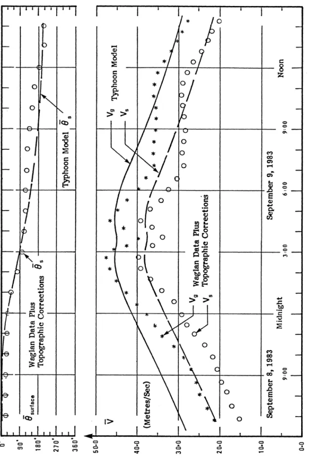
The windfield model has been checked by obtaining actual wind traces from tropical cyclone events and comparing them to the wind speeds predicted by the model. One such example is shown in Figure B.1 comparing model speeds with those obtained from the Waglan Island anemometer station during the passage of typhoon Ellen through the Hong Kong area in September 1983. It can be seen that the match of model speeds with actual recorded speeds is particularly good at the time that the maximum winds occurred.

In a study following the passage of Hurricane Alicia through Texas in August 1983, the simulation windfield model was used to recreate the time history of winds experienced in downtown Houston utilizing actual meteorological data obtained during the passage of the storm (central pressure, storm speed, etc.). In a unique set of circumstances, an accelerometer record was obtained during the most intense part of the storm for a 300 metre high-rise tower which had undergone detailed wind tunnel testing at this Laboratory. The model time history of Alicia's winds were combined with the wind tunnel test results, and the resulting predicted accelerations were compared to the actual recorded ones, as shown in Figure B.2. The agreement is seen to be excellent and adds considerable confidence to the continuing calibration that the windfield model has undergone.

B.4

The Wind Climate for a Particular Site

For most locations, a 500 kilometre simulation circle around the site is used. Historical data of hurricanes within this circle are examined to determine probability distributions of the relevant parameters for the simulation. A summary of the parameters required by the simulation is given in the table below. A time period of several thousand years is typically used for the simulation.

(26)

Statistical Simulation Parameters

Parameter Distribution Annual Occurrence Rate

Central Pressure Difference (mbars) Radius to Maximum Winds (km) Translation Velocity (m/s)

Minimum Approach Distance (km) Approach Angle (degrees)

Poisson Weibull Log-Normal Log-Normal Polynomial Von Mises

As a simulation proceeds, a separate record is kept of all wind speeds and their respective directions (the "parent" distribution) as well as the individual peak wind speeds recorded for each tropical cyclone generated (the "extreme" distribution). These distributions are fitted independently using standard maximum likelihood estimating techniques. The results are a probability distribution of wind speed and direction and a graph of extreme wind speed versus return period.

References

(B-1) Russell, L.R. and Schueller, G.F., "Probabilistic Models for Texas Gulf Coast Hurricane Occurrences", J. Pet. Tech., March 1974.

(B-2) Tryggvason, B.V., Surry, D. and Davenport, A.G. "Predicting Wind-Induced Response in Hurricane Zones", Journal of the Structural Division, ASCE, Vol. 102, No. ST12, Proc. Paper 12630, December 1976, pp 2333-2350.

(B-3) Batts, M.E., Cordes, M.R., Russell, L.R., Shaver, J.R. and Simiu, E., "Hurricane Wind Speeds in the U.S.A.", NBS Building Series 124, Nat. Bur. of Standards, Washington, D.C., 1980.

(B-4) Georgiou, P.N., Davenport, A.G. and Vickery, B.J., "Design Wind Speeds in Regions Dominated by Tropical Cyclones", Journal of Wind Engineering and Industrial Aerodynamics, Vol. 13, No. 1, December 1983 (presented at 6th International Conference of Wind Engineering, Brisbane, Australia, March 1983).

(B-5) Martin, G.S., "Probability Distributions for Hurricane Wind Gust Speeds on the Australian Coast", Proc. I. E. Aust. Conf. on Appl. Probability Theory to Structural Design, Melbourne, 1974. (B-6) Gomes, L. and Vickery, B.J., "On the Prediction of Tropical Cyclone Gust Speeds Along the

Northern Australian Coast", Inst. Eng. Aust. C.E. Trans., CE 18, Vol. 2, pp. 40-49, 1976.

(B-7) Tryggvason, B.V., "Computer Simulation of Tropical Cyclone Wind Effects for Australia", Wind Engineering Report 2/79, Department of Civil and Systems Engineering, James Cook University, Townsville, Australia, 1979.

(B-8) Georgiou, P., Mikitiuk, M.J., Surry, D. and Davenport, A.G., "The Wind Climate for Hong Kong", The University of Western Ontario, Engineering Science Research Report, BLWT-SS2-1984. (B-9) Vickery, P.J. and Twisdale, L.A. (1995), “Prediction of Hurricane Wind Speeds in the United

States”, Journal of Structural Engineering, Vol. 121, No. 11, pp. 1691-1699.

(B-10) Vickery, P.J., Skerlj, P.F. and L.A. Twisdale (2000a), “Simulation of Hurricane Risk in the U.S. Using and Empirical Track Model, Journal of Structural Division, ASCE, October.

(B-11) Vickery, P.J., Skerlj, P.F. Steckley, A.C. and L.A. Twisdale (2000b) “A Hurricane Wind Field Model for Use in Hurricane Wind Speed Simulations”, Journal of the Structural Division, ASCE, October.

(B-12) Twisdale, L.A. and P.J. Vickery (1993), “Uncertainties in the Prediction of Hurricane Windspeeds”, Proceedings of Hurricanes of 1992, ASCE, pp. 706-715, December.

(27)

(B-13) Georgiou, P. "Design Wind Speeds in Tropical Cyclone-Prone Regions", Ph.D. Thesis, Faculty of Engineering Science, University of Western Ontario, 1985.

(28)

FIGURE B.1 COMP ARIS O N OF TYPHOON WIND SPEEDS AT

WAGLAN ISLAND TO MEAS

URED DATA CORRE CTED FOR TOP O G RAP HIC EFF E CTS

(29)

FIGURE B.2 PREDICTED PEAK ACCELERATIONS FOR THE ALLIED BANK DURING HURRICANE ALICIA

(30)

APPENDIX C

THE MEASUREMENT AND PREDICTION OF SURFACE PRESSURE

C.1 Experimental

Technique

Measurements of wind-induced surface pressure at a point are accomplished by allowing the surface pressure to act on a transducer which provides an electrical analogue of the pressure. The electrical signal is digitized and then stored in its entirety for later processing.

In practice, the transmission of the surface pressure to the transducer is complicated in two ways. First, there are usually a large number of measuring positions, requiring the use of a large number of transducers. Secondly, the model is generally too small to allow the transducers to be very close to the measuring locations. The resulting use of relatively long lengths of pneumatic tubing leads to a modification of the pressure at the transducer compared to that at the model surface.

These problems are dealt with as follows: pressure taps on the model are connected pneumatically to electronic pressure scanning modules, each capable of handling 16 different taps. The modules use internal multiplexers which are sequentially scanned at a selectable fixed scan rate. The maximum rate that a particular input can be scanned is inversely proportional to the number of inputs on each module; 16 inputs were considered optimal for wind engineering applications at the BLWTL. The sampling rate is typically 400 or 500 samples per second per input. All modules are synchronized and the 16 outputs from each module are time-shifted analytically so that the signals from all taps can be considered simultaneous.

The pneumatic connection between model and scanning module is typically 1/16”ID plastic tubing containing a restricting insert of small bore at a specific point along its length. The function of the restrictor is to add damping to the resonant system made up of the pressure tube and the connecting volume adjacent to the pressure transducer. The resulting pressure system with about two-foot long tubes responds with negligible attenuation or distortion of surface pressure fluctuations with frequencies up to about 200 Hz. Although some response is obtained for signals of several hundred Hertz, these higher frequencies suffer increasing attenuation.

The data acquisition system records the digitized signals from the scanning modules at the set scanning rate (typically 400 Hz). Typically, sampling is continued for a period of up to about a minute in real time (see Section C.3). The reference dyn