Segment phoneme classification from speech under noisy conditions: Using amplitude-frequency modulation based two-dimensional auto-regressive features with deep neural networks

(1)

Segment phoneme classification from

speech under noisy conditions:Using

amplitude-frequency modulation based

two-dimensional auto-regressive features

with deep neural networks

School of Electrical Engineering

Thesis submitted for examination for the degree of Master of Science in Technology.

Espoo 03.08.2016

Thesis supervisor:

Prof. Paavo Alku

Thesis advisor:

(2)

Author: Rijuban Rangslang

Title: Segment phoneme classification from speech under noisy conditions:Using amplitude-frequency modulation based two-dimensional auto-regressive features with deep neural networks

Date: 03.08.2016 Language: English Number of pages: 6+64

Department of Signal Processing and Acoustics

Professorship: Speech communication technology Code: S-89

Supervisor: Prof. Paavo Alku Advisor: Dhanajaya Gowda(Ph.D.)

This thesis investigates at the acoustic-phonetic level the noise robustness of fea-tures derived using the AM-FM analysis of speech signals. The analysis on the noise robustness of these features is done using various neural network models and is based on the segment classification of phonemes. This analysis is also extended and the robustness of the AM-FM based features is compared under similar noise conditions with the traditional features such as the Mel-frequency cepstral coefficients(MFCC).

We begin with an important aspect of segment phoneme classification experiments which is the study of architectural and training strategies of the various neural network models used. The results of these experiments showed that there is a differ-ence in the training pattern adopted by the various neural network models. Before over-fitting, models that undergo pre-training are seen to train for many epochs more than their opposite models that do not undergo pre-training. Taking this difference in training pattern into perspective and based on phoneme classification rate the Gaussian restricted Boltzmann machine and the single layer perceptron are selected as the best performing model of the two groups, respectively.

Using the two best performing models for classification, segment phoneme classi-fication experiments under different noise conditions are performed for both the AM-FM based and traditional features. The experiments showed that AM-FM based frequency domain linear prediction features with or without feature compen-sation are more robust in the classification of 61 phonemes under white noise and 0 dB signal-to-noise ratio(SNR) conditions compared to the traditional features. However, when the phonemes are folded to 39 phonemes, the results are ambiguous under all noise conditions and there is no unanimous conclusion as to which feature is most robust.

Keywords: Robust speech recognition system, AM-FM based features, Neural networks

(3)

Preface

This thesis work is undertaken for fulfillment of the requirements of the Master’s Degree Program in Communications Engineering at Aalto University School of Electrical Engineering, Finland. The task was performed at the Department of Signal Processing and Acoustics, School of Electrical Engineering, Aalto University.

First and foremost I would like to express my sincere gratitude to Prof. Paavo Alku for giving me an opportunity to work with him and his team. Secondly, I would like express my gratitude to my instructor Dhananjaya Gowda for all the encouragement and advice he has given me throughout the course of the thesis. I would also like to thank Bajibabu Bollepali for giving me valuable advice pertaining to the subject of neural networks. I would also like to thank all the staff members that are responsible in maintaining the triton accounts and also Tarmo Simonen for helping me out with all the IT related issues. I would also like to thank all my colleagues and friends who were part of the foosball games in the piano bar.

Lastly, I would like to thank my family especially my sister for being my constant source of inspiration and support these last couple of years.

(4)

Symbols and abbreviations

Hj(x) Neural network posterior probability at output unit j for inputx

E(v, h) Energy function of a joint configuration of visible and hidden units

EAE Error function of an auto-encoder

Esparse Error function of a sparse auto-encoder

ECAE Error function of a contractive auto-encoder

H(z) Transfer function of a simple resonator

Ai[n] Amplitude modulation component of the ith narrowband signal

Error(h, S) Segment phoneme classification error

RASTA Relative spectra

MLLR Maximum likelihood linear regression

MAP Maximum a-posterior

MCE Minimum classification error

MMI Maximum mutual information

LP Linear prediction

ASR Automatic Speech recognition

AM-FM Amplitude modulation-frequency modulation

AM-FM FDLP AM-FM Frequency domain linear prediction

AM-FM 2D AR AM-FM two dimensional auto-regressive

MFCC Mel-frequency cepsral coefficient

PLP Perceptual linear prediction

MLP Multi-layered perceptron

ReLU Rectified linear unit

GRBM Gaussian Restricted Boltzmann machine

GPU Graphic processor units

PCA Principal component analysis

DNN Deep neural networks

GMM/HMM Gaussian mixture models/Hidden Markov models

CMN Cepstral mean normalization

(7)

1 Introduction

1.1 Overview

Over the last few decades automatic speech recognition system(ASR) has undergone considerable improvement. This has lead to widespread use of the technology in areas such as automated call centers, personalized assistant in mobile phones, hands free computing, speaker dependent recognition system in many home automated appliances, etc. However, the inability of the automatic speech recognition system to reach human level performance has restricted its coverage. This is especially true in areas such as defense systems where the margin of error is small.

The performance of the speech recognition system further aggravates under noisy conditions. Noise influences the speaker as well as the system. The noise corrupts the speech signal and also leads to the Lombard effect [1]. The Lombard effect results in changes to the pitch, the duration and amplitude of syllables. Most speech recognition system are inherently designed or trained under clean conditions [2]. Hence, such changes to the input speech leads to substantial degradation in the performance of the automatic speech recognition system.

Various speech enhancement techniques are used to reduce the effect of the noise. With additive noise speech enhancement methods include Wiener filtering [3], power bias subtraction [4] and missing data reconstruction [5]. For convolutive noise, methods such as feature warping [6], RASTA processing [7] and cepstral mean subtraction [8] are often used. As for acoustic models, models that are derivative of Gaussian mixture models and trained generatively are made to adapt to the noise environment using adaptation technique such the maximum likelihood linear regression(MLLR) [9] and maximum a posterior(MAP) [10]. Discriminative trained acoustic models on the other hand are adapted using minimum classification error(MCE) [11] and maximum mutual information(MMI) [12] .

Most of the speech enhancement technique mentioned work by assuming the type of noise and estimating the noise properties. Hence, these methods do not generalize well to other types of degradations [13]. Similarly with the models, the adaptation techniques mentioned are trained using data that represent a subset of the test set domain. But collecting a reasonable amount of data for all test conditions is not always possible. Thus, to ensure an all round robustness in the system, signal analysis techniques for feature extraction should concentrate on regions less affected by noise. Also, the system should adapt and generalize well to all test conditions even when trained using clean speech signal.

Over the years a considerable amount of research has been done to arrive at signal analysis techniques that are robust under various degradation conditions. These methods involve modeling the speech signal in terms of its envelope and phase modulation and are known as the AM-FM model of speech [14]. Improvements are reported in [15] for various speech recognition task when using features that are derivative of the auto-regressive modeling of the envelope of the speech signal.

From the model point of view, deep neural networks(DNN) have replaced Gaussian mixture models in the acoustic model of the ASR system. Such acoustic models

(8)

achieved considerable improvement compared to Gaussian mixture models with respect to various speech recognition task. Using deep neural networks have led to improvement in phoneme recognition as reported in [16]. Deep neural networks without any form of adaptation are also extended to modeling of robust acoustic models. This is achieved by a different training approach such as multi-condition training. The deep architecture allows the discovery of representations that are stable to variations in the input signal as discussed in [17]. Deep neural nets are also trained as de-noising auto-encoder and used for speech enhancement [18]. Overall there has been considerable improvement in the speech recognition system under noisy conditions using such deep neural networks.

1.2 Objective

The objective of the thesis is to study the robustness of the AM-FM based features under different noise conditions. This study uses various neural network models and is based on segment phoneme classification experiments. We begin with an important aspect of segment phoneme classification experiments which is the study of the functionality of various neural network models with regards to classification. The various neural network models used can be divided into two groups. The first group include networks which do not undergo any initial pre-training such as the single layer perceptron and the multi-layered perceptron(MLP) with rectified linear(REL) units that are integrated with a model averaging technique called the dropout. Also included are neural networks models that are initially pre-trained as stacks of restricted Boltzmann machine and auto-encoder before being fine-tuned as an MLP for classification.

After the study of the functionality of the various network models we choose based on the phoneme classification rate the best neural network models; one from each group. These neural networks models serves as network classification models that are used in studying the robustness of the AM-FM based features under different additive degradation. The degradation types included are the white, babble and factory noise with signal-to-noise(SNR) ratio of 0,10 and 20 dB. The study is also conducted using features that are compensated with RASTA filtering. Also, the robustness of the AM-FM based features with regards to phoneme classification is also compared under similar conditions with the traditional features. The AM-FM based features included are the AM-FM FDLP and the AM-FM 2D AR features. The traditional features used include mel-frequency cepstral coefficients(MFCC) and the perceptual linear prediction(PLP) features.

(9)

2 Introduction on feature extraction and pattern

classification

2.1 Overview

The process of transcribing speech features to words in a speech recognition system happens at three levels. The first involve using various signal processing techniques for extracting speech features. Secondly, the acoustic model establishes at the acoustic-phonetic level the relationship between the features and the smallest linguistic unit namely, the phoneme. This in turn is used when representing larger speech units such as words or phrases. Finally, the language model decides on the sequence of words. In this chapter, we will review the front-end method of feature extraction. We will also look at an important aspect of the acoustic model which is the mapping of the features to the respective phonemes.

2.2 Feature Extraction

The first step in an automatic speech recognition system involves pre-processing of the speech signal and extracting discriminative features. These discriminative features are representative of the speech characteristics that are stable over time and remain unaffected by reasonable background noise. These features also represent speech characteristics that are discriminative between speaker while being tolerant to intra-speaker variability such as health and emotion. Most state of the art features do not incorporate all of these speech characteristics. For research and certain practical conditions, features that partially represent these speech characteristic are considered [19]. The most popular features include the mel-frequency cepstral coefficients(MFCC) and the perceptual linear predictions(PLP) features. Here, to give an example to the generation of speech feature we will discuss the generation of the MFCC features.

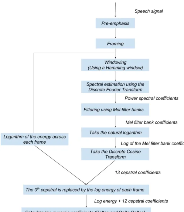
Speech is the sound generated as it gets filtered through the vocal tract including the tongue and teeth. The vocal tract manifest itself in terms of the short-time power spectrum envelope. MFCC represent to a certain accuracy the envelope of the power spectrum [20]. There are usually 39 dimensions in the MFCC feature vector. These include 12 static features, 1 energy feature, the first and second order derivative of the static features [21]. The procedure for extraction of MFCC is summarized as follows.

1. Pre-emphasis :- The spectrum associated with speech signal decreases at a rate of −20dB per decade. Thus, high frequency regions of the speech signal have smaller amplitude [22]. Pre-emphasis is intended to offset this natural slope of the speech spectrum by flattening out the spectrum of the speech signal [23]. Pre-emphasis is achieved by filtering the speech signal through a finite impulse

(10)

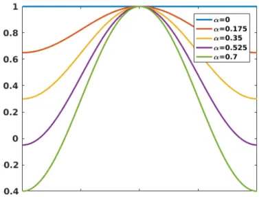
Figure 1: Hamming window

response(FIR) filter defined as shown below

Hpre(z) = 1 +az−1 (1)

where the typical range for a is [−1.0,−0.4].

2. Framing :- The human speech signal represent a slowly time-varying signal [21]. Under short time frames, it is treated as a stationary process [24]. This treatment of the speech signal as a stationary time process is essential for the spectral analysis of the speech signal. Normally, the frame size is considered to be20−40mswith an frame step of10ms. If we consider a speech signal sampled at 16000Hz, a frame size of25mswill result in a frame of0.025×16000 = 400 samples. A frame-step of10ms will result in 160 samples. There is an overlap with the first frame extending from 0-400 samples, while the next frame starts at 160 and extend for another 400 samples.

3. Window:- Windowing serves as a necessary pre-cursor before the spectral analysis using Fourier transform. The Fourier transform assumes a finite set of data that is one period of a periodic signal. Thus, there is a circular topology with the beginning and the end point of the signal being connected. However, if such conditions are not met and the signal is discontinuous, these discontinuities show up as high frequency component in the Fourier transform [25]. To prevent this, the signal is filtered using a window function. The most commonly used window in speech signal analysis is the Hamming window which is defined by w(n) as shown below:

(11)

Figure 2: A sketch of the mel-filter bank

where different values of α correspond to different curves for the Hamming window and the window length is N+ 1

4. Discrete Fourier transform to each frame :- After windowing, the samples present in each frame are converted from the time domain to the frequency domain. This spectral analysis of each frame is achieved using the fast Fourier transform(FFT). These frequency domain coefficients are complex numbers that are representative of the magnitude and the phase of the speech signal. In the case of the MFCC, only the magnitude of the spectral coefficients is considered [21].

5. Mel filter-banks:- Human hearing is not equally sensitive to all frequency bands. To incorporate this non-linear perception of frequency, the spectrum of the speech signal is filtered by a group of triangular banks. These mel filter-banks are arranged on a mel-frequency scale. The relation between mel-scale frequencies to the linear scale frequencies(Hertz) is given by

fmel = 2595 log(1 +f /700) (3)

wherefmel andf is the frequency in the mel-scale and linear scale, respectively.

On the mel-scale the windows are evenly distributed. The bandwidth of such windows are narrow at low frequencies and gradually increases as it approach the higher frequencies regions. In order to get an estimate of the amount of energy in each filter bank, the spectrum is multiplied with the triangular filter and the coefficients in each of the filter bank are added [21].

6. Applying the natural logarithm:- The human auditory system also exhibit non-linear loudness characteristics. This is approximated in the feature extraction method by considering the logarithmic scale. Also, using this logarithm scale

(12)

ensures that the convolutive distortion is additive and can be removed using simplified speech enhancement techniques.

7. Discrete cosine transform :- The discrete cosine transform is meant to de-correlate and convert the log-mel spectrum back to the time domain. This time domain representation represent the MFCC features. Only a fraction of the de-correlated Mel coefficient are considered for feature extraction.

8. Log energy :- The Log energy is calculated directly from the time domain. It represent the energy of each frame. The log energy sometimes replaces the0th

cepstral coefficient for various speech recognition task.

9. Delta and the delta-deltas:- The MFCC coefficients described so far represents only the power spectral envelope of the speech signal [20]. However, the speech signal also has information that is loaded in the trajectories of these coefficients over a period of time. These trajectories are calculated in terms of the delta coefficients that are defined as

dt= PN

n=1n(ct+n−ct−n)

2PN_n₌₁n2 (4)

where dt is the delta coefficient computed from frame t. It is computed in

terms of the static cepstral coefficients ct+n to ct−n. A typical value of N = 2.

Delta-deltas coefficients are calculated using the same formula as shown above, replacing the static coefficients with the delta coefficients. These dynamic speech features are appended to the static features and used in various speech recognition problems.

(13)

Figure 3: Flowchart showing the step by step process in the extraction of MFCC features

(14)

2.3 Statistical pattern classification

Since the start of speech recognition research many methods for transcribing speech to words have been proposed. These include template matching and statistical methods based techniques. In template matching techniques a prototype or a pattern of the speech utterance(usually of a 2-D shape) is available. Template matching involves a direct comparison between the unknown pattern and the training pattern taking into account all available pose such as translation, rotation and scale changes [26]. Statistical methods on the other hand include well formulated probabilistic mathematical models. These mathematical models are particularly suitable for speech recognition system as they can model the uncertainty or incomplete information that can arise from contextual effects,confusable sound etc. [27]. Statistical methods such as the Hidden Markov Model continue to be in use even today delivering commendable results on many aspect of speech recognition.

An important aspect of speech recognition considered in this thesis is that of phoneme classification. Phoneme classification is described as the task of tagging a speech utterance to its respective phoneme. Various statistical methods are considered for phoneme classification. The Elena project represent one such study where using real world datasets statistical methods such as the neural networks are used for task of phoneme classification [28].

In the coming section we give an overview of various classification methods. We begin with the Bayesian classification methods. We then proceed to discussing neural networks and also deep neural networks based classification.

2.3.1 Bayesian Classification

The Bayesian classification approach forms the basis of many statistical classification methods. Based on the objective of establishing decision boundaries Bayesian classification methods can be sub-divided into two section. The probabilistic and the discriminant analysis classification approach. In the probabilistic approach, the class conditional probability distribution of a pattern is estimated. Then a discriminant function that specifies the decision boundaries is established. A number of decision rules is associated with the probabilistic approach. These include the Bayes decision rule, the maximum likelihood and the Neyman-Pearson rule. Most of the decision rule are derivatives of the Bayes decision rule but have distinct training strategies [28].

The discriminant analysis approach establishes the decision boundaries directly and is supported by Vapnik’s philosophy. Vapnik’s philosophy states that it is better to solve the problem directly rather than considering an intermediate step especially if there exist a limited amount of information for solving the problem. The discriminant analysis approach follows a parametric form of the decision boundary. The parameters of the decision boundary are estimated by minimizing a cost function [26]. The cost function can be an error criteria such as the mean square error between the true class assignment values and the predicted class values.

(15)

In the coming section we begin with an explanation of the probabilistic approach and consider the Bayes decision rule and the likelihood decision rule. Then we proceed to explaining discriminant analysis approach for classification.

The Bayes decision rule approach can be summarized as follows: Consider that a given feature vectorx= (x1, x2, ..., xd) of d dimensions that needs to be assigned

to one of the c categoriesw1, w2, ..., wc. If P(wj)is the prior probability of group j

and P(x|wj)is the probability density function . Then as per Bayes’ rule

P(wj|x) = P(x|wj)P(wj)

f(x) (5)

where P(wj|x) is the posterior probability of group j and the marginal distribution

f(x) =PC_i₌₁f(x|wj)P(wj).

The training step for the Bayes decision rule involves estimating the class condi-tional densities P(x|wj) from the training data. A classic parametric approach is

to model the class conditional densities as multivariate normal distributions or as a mixture of some standard probability densities. Hence, the training step involves estimating the parameters of the density function using the maximum likelihood approach or using the expectation maximization algorithm for the mixture models. In the non-parametric case, the k-NN method represents a popular non-parametric density estimation. After estimating the parameters of the class conditional densities and assuming that prior for each classP(wj)is known, the Bayes decision rule assigns

the input feature vectorxto a class wi with the minimum misclassification risk. The

class dependent misclassification risk is defined as shown below R(wi|x) =

c X j=1

L(wi, wj)∗P(wj|x) (6)

whereL(wi, wj)is the loss incurred in decidingwi when the true class iswj. Thus

as per the Bayes decision rule, feature vectorx is assigned to a class wi when

R(wi|x) =mini=1,2,...CR(wi|x) (7)

In the case of the 0/1 loss function where each class misclassification is assumed equal then L(wi, wj) =    0, if i=j 1, if i6=j

The Bayes decision rule simplify to equation(8) with the feature vectorxassigned to classwi when

P(wi|x)> P(wj|x) f or all j 6=i

or

P(x|wi)P(wi)> P(x|wj)P(wj)

(8)

This represent the optimal Bayes decision rule with the vector xassigned to a class with the maximum posterior probability.

(16)

For the explanation of the maximum likelihood decision rule, we again assume that the feature vector x needs to be assigned to one of thec class w1, w2, ..., wc.

The likelihood decision rule is an extension of the Bayes rule with a 0/1loss function. It also makes an assumption that the prior P(wj) across all the classes are equal.

Thus, the decision rule allocates the feature vector x according to equation(8) with the decision rule dependent on the posterior probability [29]. The training step for the maximum likelihood rule aims to estimate this posterior probability directly. For a parametric maximum likelihood method such as the linear or logistic regression, the parameters that can define the posterior probability are estimated using the gradient descent method with a least square or cross entropy criterion fitting function. The cross entropy criteria is preferred as it considers a binomial distributed error. Also, the categorical cross entropy is extended to multi-class classification problems with the posterior probability modeled as a soft-max function

Discriminant analysis method makes no assumption on the conditional class probability density. The Fisher linear discriminant analysis method as described in [30]represent one such method. The Fisher linear discriminant finds a linear projection wT_x_{for the training data} _x_{, with}_w _{being the linear transformation matrix. This}

linear function aims to maximizes the ratio of the between class separation to the within class separation and is thus derived by maximizing the following objective function J(w) = argmax w wTSBw wT_S Ww (9) where SB is the between class scatter matrix" andSW is the "within class scatter

matrix". The definition of the scatter matrix are SB = X i (µi−xˆ)(µi−xˆ)0 SW = X i X jc (xj −µi)(xj −µi)T (10)

where xˆ is the overall mean of the data.

For a feature vector xthat is to be classified to one of thecclasses w1, w2, ...., wc.

The average score wT_µ

c is calculated for each of the class i = 1, ....c.The decision

rule assigns the feature vector xto class wj when

|wTxˆ−wTµi|<|wTxˆ−wTµj| f or all i6=j (11) 2.3.2 Neural network based classification

Statistical models discussed so far are built on the Bayes Decision theory which considers calculating the posterior probabilities using various training strategies. Most of the statistical classification techniques have an underlying assumption of the conditional class and prior distributions. These techniques generally prevail when the model assumptions and underlying conditions are met.

Neural networks have emerged as an important alternative to traditional statistical models. Neural network unlike statistical models make no assumption regarding the

(17)

conditional class and prior distribution [29]. A neural network for classification can be defined as a mapping function H : x → y of a feature vector x to the output vectory. This mapping functionH as per the least square estimation theory is given by

Hj(x) = E[yj|x] (12)

where E[yj|x]is conditional expectation of yj givenx.For a binary output vector y

with a jth basis vectorej = (0, ...,1,0, ...,0) if x class wj the mapping function is

defined as the posterior probability as shown below

Hj(x) =E[yj|x] =P(wj|x) (13)

where P(wj|x) is the posterior probability of the class wj given x.

Neural networks are also universal approximators. As already stated neural networks provide estimates of the posterior probability. An explicit connection between the neural networks and the traditional statistical classifiers is arrived based on the posterior probabilities. Neural networks as discussed in [31] are equivalent to seven statistical classifier including the Fischer linear discriminant, the minimum empirical error classifier etc.. Also, neural network that are trained to minimize the cross-entropy cost function approximate the logistic regression model. Thus, neural network can approximate the posterior probability distribution and also bears resemblance to many statistical methods.

In the coming section we will begin with a definition of a neural network. Then proceed towards the various architectures and different training algorithms associated with each architecture. Then we will review deep neural networks and finally address the issue of learning and generalization that is normally encountered while training neural network.

Basic definition of an artificial neural network

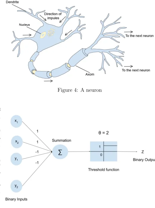
Human beings have an inherent ability to easily recognize patterns. This ability has drawn scientist to design recognition systems that are inspired by the human cognitive system. An artificial neural network represent one such system. The basic units in an artificial neural network are the artificial neurons. Artificial neurons are highly abstract model of the natural neurons shown in Figure.4that constitute the human cognitive system. Such an abstract model of the artificial neural network helps at discovering characteristics of the neurons that are most cognitively relevant.

The first model of the artificial neuron was presented by physiologists, McCulloch and Pitts in 1943. This neuron model considers unweighted or fixed excitatory or inhibitory connections between the binary inputs and outputs. For an input signalx1, x2, ....xnandy1, y2, ..., yn appearing at the excitatory and inhibitory input

connections respectively. The neuron unit is evaluated based on the following decision rule

:-• A single inhibitory signalyi = 1deactivates the neuron and result in a0binary

(18)

Figure 4: A neuron

Figure 5: Mc Culloch and Pitts neuron with output = 1 whenP

i=1xi ≥θ = 2 with

yi = 0 else output = 0 with yi = 1

• If yi = 0 for all i= 1, ..., nthen only excitation input connections is considered.

The total excitation x=x1+....+xn is compared with the thresholdθ. The

neuron is activated only with a binary output1 if and only if x≥θ.

This neuron model is biologically relevant as it is models the electrochemical process that goes on inside a natural neuron [32]. Also, under different threshold considerations this neuron resembles most logic circuits.

(19)

Figure 6: Single layer perceptron.

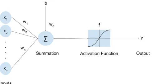
beginning. The concept of ’learning’ is not available for such kind of neuron model. To improve upon this Rosenblatt in 1958 developed the perceptron neuron model. In the classic perceptron model weights are introduced which are adjusted using a trial and error method. Minsky and Papert made further improvement to the classical perceptron model. The model in Figure.6represent the perceptron model introduced by Minsky and Papert. Mathematically this model can be represented as shown below y=f( n X i=1 wixi+b) (14)

where wi are the adjustable weights, xi are the inputs, f is the activation function

and b is the bias

An essential element of the perceptron model seen in Figure.6is the introduction of the activation function. The activation function allows the neuron to be able to generalizes and solve different kinds of problem. The neuron is made to resemble the McCulloch and Pitts neuron when a binary activation function is used. Activation functions such as the differentiable sigmoid activation has led to the development of various learning methods for the perceptron. Learning methods such as the least mean square and the back-propagation algorithm are possible because of the differentiable activation functions. Another key feature of the activation function is that it provides a probabilistic set-up for the neuron by projecting the output values within ranges [0,1][33]. Lastly, the activation function also introduces non-linearity in the neuron which has helped in mapping the non-linear relationship between the inputs and the outputs.

(20)

Neural network Architecture

Neural networks have been applied to many real world classification problems. These include application in speech recognition [[34],[35]], medical diagnosis [36] etc.. The scope of neural network architecture for classification can extends to many different type. These include network architecture such the single layer perceptron, the multilayer perceptron [36], competitive models such as the self-organizing maps [37], recurrent networks [34] and energy based Hop-field networks.

Figure 7: Multi-layer perceptron

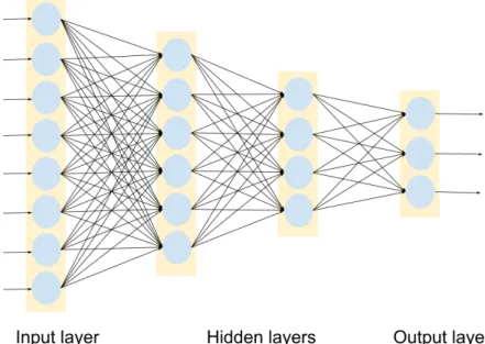
The multi-layered perceptron with its feed-forward architecture is commonly used in classification problems. This network shown in Figure.7consist of an input layer, one or more hidden layers and an output layer. The neuron in each layer are not connected to each other. The flow of information is unidirectional with the input undergoing a series of non-linear transformation from the input layer to the output layer.

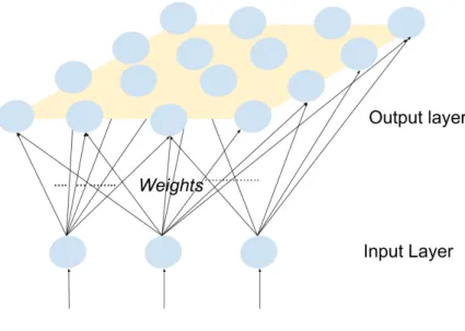
Self organizing maps shown in Figure.8is a fully connected single-layer network with the output layer organized in a two dimensional arrangement of nodes [37]. Using a soft competitive learning algorithm the high dimensional input is mapped to the two-dimensional array of node. Generally the self organizing map network is not intended for classification. However, in the presence of class specific data self organizing maps with the learning vector quantization can be used for classification.

Hopfield networks are symmetrically connected recurrent networks with binary units as shown in Figure.9. These binary units serves both as input as well as the output units. Hopfield nets are defined by the configuration of the binary units which is reflected in the energy function. Under stable binary configuration and minimum energy they serve as associative memories with the network able to memorize certain states and patterns [32]. An extension of the Hop-filed network is the restricted

(21)

Figure 8: Self organizing maps

Figure 9: Hopfield networks

Boltzmann machine. The restricted Boltzmann machine considers hidden binary units while serving as associative memories. Restricted Boltzmann machines form the basis of the early deep learning research suggested by Geoffrey Hinton back in 2006. These machines when fine-trained as a multi-layered perceptron can perform classification.

(22)

Training methods in neural networks

The neural network architectures presented in the previous section were all seen to solve the classification problem. The presence of different neural network architecture has necessitate the formulation of different training methods. However, these training methods are mostly derived from the Hebbian learning rule. This Hebbian learning rule generally allows to fine-tune the variable weights between the network units in each of their respective networks.

The Hebbian learning rule is defined as follows. If two network units i andj are considered, as per the Hebbian rule the connection weightwij is strengthen when the

two units i and j are simultaneously active. Thus, if the network is directed from i toj. The Hebbian learning rule updates the weightwij as shown below

∆wij =γxixj (15)

where γ is the learning rate, with xi andxj are the network unit values of units i

and j respectively.

The Hebbian learning rule presented in equation(15) is considered unstable. There is no threshold level to the increase of the weight wij between the units i and the

unit j. The Oja’s learning rule is an improvement of the Hebbian learning rule and is defined as shown below

∆wij =γxi[xj−wijxi] (16)

Thus in equation(16) while the first update term follows the Hebbian learning, the other serves as a regulator keeping the norm of the weight vector wij close to

unity.

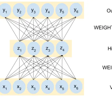
Learning in a neural network can also be achieved by optimizing the loss function. Such learning methods are associated with multi-layer perceptron models and include the back-propagation algorithm. The back-propagation algorithm is an instantaneous stochastic gradient algorithm which tries to minimize the mean-square error between the desired output and the real output. Let us consider a multi-perceptron model with two hidden layers as shown in Figure.10. The network consist of three layers. The first layer is between the input and the first hidden layer, the second layer between the two hidden layers and the third between the hidden layer and the output.

W(k), f(k), v(k) =Wkx(outk−1), x

(k)

out =f(k)(v(k)) for k = 1,2,3 are the weights,

acti-vation function, linear response and output associated with each of the three layers. Also, the weight W(k) _{for each of the}_k _{layers consists of units} _w(k)

ij which represent

connection weights between element i of layerk−1 and element j of layer k. For an training pair{x, d}, the output of the network is given as shown below

y =f(3)[W(3)f(2)[W(2)f(1)[W(1)x]]] (17)

where y is the output of the network. Hence, the mean square error between the desired responsed and the output y is given by

JM SE =

1

2{||d−y||

2_}

(23)

Figure 10: Multi-layer perceptron

Using the gradient descent approach for the mean square error, the update rule for a weight w_ji(k) in any of the k layers, is as shown below

∆w_ji(k)=−µ(k)∂JM SE

∂w(_ijk) (19)

where µ(k) is the learning parameter.

The update rule can also be defined in term of the local error. To give a clear definition of this local error, assume a component of the input vectorxi is present

on theith neuron of the first layer. The local error is defined as shown below δ_j(3) = ∂JM SE

∂v(3) = (dj −yj)g(v (3)

j ) (20)

whereg is the derivative of the activation functionf. In general for the hidden layers the local error is given by

δk_j = (

nk+1 X h=1

δ_h(k+1)w_hj(k+1))g(v_jk) (21)

Thus, the update rule for the weights in all the layer is as shown below

∆w(_jik) =µ(k)δ_j(k)x(_out,ik−1) (22)

The cost function defined by the mean square error leads to a regression model where the errors are normally distributed with the update rule being susceptible to a

(24)

learning slowdown[28]. Thus, in most cases the multi-layered perceptron is trained considering the cross-entropy cost function. This cost function uses a statistically correct binomial distributed error and is resistant to a learning slowdown [29]. The cross-entropy cost function is defined as shown below

JCross−entropy = X

j

dj log(yj) (23)

where d is defined as a basis vector and the output yj for the perceptron model

shown in Figure.10is as shown

yj =

exp(v_j3)

Pc

j=1exp(v3j)

(24)

where c is the number of output neurons with the output activation functionf(3) _of

the perceptron model defined as a softmax function.

Neural networks such as the multi-layer perceptron discussed above are referred to as 0shallow0 networks. The absence of a proper training algorithm limits their size to not more than two layers. If we consider a network with many hidden layers, the back-propagation algorithm would progresses extremely slow from one layer to the next. It would halt altogether without making an significant update on the weights[38].

In the coming chapter we will look at efficient ways of training neural networks with many hidden layers. These networks with their respective training algorithms are meant to overcome the under-fitting problems associated with the gradient descent algorithm [39]. We will consider using energy based stochastic Hopfield networks, auto-associators networks etc in training deep neural networks.

(25)

2.3.3 Deep neural networks based classification

Neural network models can approximate any function to any level of precision.

0_Shallow0

network models however require more hidden units and are less efficient in approximating such functions. Deep neural network are coherent with the complexity theory of circuits. A deeper neural networks architecture ensure an efficient model both in terms of the number of parameters and elements required to represent functions. Evidence also suggests that deep networks with many levels of non-linearity can handle more complex task provided, there is enough data to capture the complexity [38].

From the AI perspective, the goal is to develop systems that can mimic the human brain in its ability to learn, sense, remember and recognize. This is translated to a AI system that can learn and represent the meaningful representation of input data [40]. 0Shallow0 networks to some extend are able to learn and solve AI problem such as classification. However, they are unable to represent features inherent to the data. Also, 0shallow0 networks cannot work with unlabeled data.

The need for algorithm that can train deep neural networks has led researches to many different network architectures. These network architectures include convolution neural network and the restricted Boltzmann machine. These network generally follow their respective training algorithm. However, a key element observed in all these architecture is the use of an unsupervised initial training [41]. This training yields a good starting point for the parameters before they are further updated based on the task at hand.

In the coming section we will look at training deep neural networks using stacks of restricted Boltzmann machines(RBM) and using stacks of auto-encoders. Both follow a similar training schedule with the auto-encoder considered easier to train than the RBM [42]. Finally, we included in this section the training of multi-layered perceptrons with has more layers than a 0shallow0 network. These multi-layered perceptron consider a activations function other than the sigmoid activation. With these activation function, the training algorithm is improved and hence such networks can be extended to many layers.

Training using Restricted Boltzmann Machines

The idea of training deep neural networks using stacks of restricted Boltzmann machines was proposed by Geoffrey Hinton in 2006. Hinton derived his inspiration from training deep belief networks from deep belief networks that also consists of stacks of restricted Boltzmann machines or auto-encoders. Hinton and his student Yee-Whye Teh made an observation describe in [43] that an individual layer of the deep belief network can be trained greedily one layer at a time in an unsupervised manner. Also the trained lower hidden layer served as input to the next sub-network. This algorithm was later extended as the first effective method to training deep neural networks.

(26)

Figure 11: Restricted Boltzmann machines

• A greedy layer wise pre-training phase one layer at a time

• A fine-tuning of the network with respect to a cost function which is dependent on the criteria of interest.

In order to describe the pre-training phase it is important to define what an RBM is and then discussed how unsupervised training is performed on the RBMs.

A Restricted Boltzmann machine shown in Figure.11 is an extension of the Hopfield networks. Besides, the layer of visible units that are not connected to each other. It also consists of un-connected binary hidden units that share an undirected symmetrical connections with the visible units. Like the Hopfield networks, the configuration of the binary units in an RBM is defined in term of an energy function. The energy function E(v, h) of a joint configuration of the visible v and the hidden units h is as shown below.

E(v, h) =−X i bivi− X j cjhj − X i X j viwijhj (25)

which is expressed in vector form as

E(v, h) = −bTv−cTh−hTWv (26)

where W represent the weight andb, c are the respective biases of the visible and hidden layer.

Energy based models such as the RBM also define a probabilistic distribution through this energy function

p(v,h) = e

−E(v,h)

Z (27)

with the normalizing factor Z also called the partition function defined as a sum over all the configuration of the visible and hidden binary units.

Z =X

v,h

(27)

Subsequently, the marginal distribution of the visible units over the hidden units is p(v) =X h p(v, h) = X h e−E(v,h) Z (29)

If we define a free energy function as shown below F(v) = −logX

h

e−E(v,h) (30)

then the marginal distribution reduces to : p(v) = e F(v) Z with Z = X v eF(v) (31)

Also, the RBM has no intra-layer connections,there is a connection only between the visible units and the hidden units. Hence, a binary hidden unit is set to 1 with the following probability for an input vectorv

p(hj = 1|v) =σ(bj + X

i

viwij) (32)

whereσ is the activation function. Similarly a visible unit is set to 1 given the hidden vector h with the following probability

p(vi = 1|h) = σ(ci+ X

j

hjwij) (33)

Energy based model can be learned by performing stochastic gradient descent on the likelihood of the training data

∂logp(v)

∂θ =E[vihj]data−E[vihj]model (34) where the E[ ]data, E[ ]model denotes the expectation over the training data and model

respectively. Thus the update rule for the weight and the bias parameter is as follows ∆θ =(E[vihj]data−E[vihj]model) (35)

Getting an unbiased sample of E[vihj]data is relatively easy. In contrast as

explained by Hinton in [44] it is difficult to get an unbiased sample fromE[vihj]model

as that the visible units are set at a random state. Generally, it takes performing alternate Gibbs sampling for a long time to get a reliable estimate of theE[vihj]model

sample. A faster and reliable training can be achieved using the contrastive divergence method. The states of the visible units are set to that of the training vector. The hidden units are computed as per equation(34). Once the hidden units states are set, a ’reconstruction’ is performed such that the hidden units are updated as per equation(35). Thus, the update rule for the parameter reduces to

(28)

Figure 12: Auto-encoder

Contrastive divergence results in overall improvement in the training even as measured in the cross-entropy term even though it just an approximation of the log-likelihood [44]. This learning rule improves greatly if more alternating steps of Gibbs sampling are considered before E[vihj]reconstruction is considered.

After the pre-training step, the network of stack RBMs is considered wholly. An extra layer is added on top of the stack RBM. Generally a softmax layer is consider for multi-class classification. The network is further fine-tuned using a gradient descent algorithm to minimize an error or cost function. A cross-entropy cost function is preferred.

Auto encoder

Deep neural networks are also trained using stacks of auto-encoders. Auto-encoder based deep neural networks undergo an initial greedy layer-wise pre-training and are further fine-tuned based on the task of interest.

An auto-encoder shown in Figure.12 is a three layer neural network consisting of an input, a hidden and an output layer. Auto-encoders are auto-association network with the input encoded in the hidden layer units. For an input vector x, the auto-encoder maps it to a hidden representation z as shown below

z=f(Wx+b) (37)

where W are the weights, b is the bias and f is the activation function. This latent representationz of the inputxis further mapped to the output layer as shown

(29)

where with tied weights i.e W0 =WT it is meant to represent a 0reconstruction0 of the input vector x.

Training an auto-encoder involves minimizing the error between the original input x and the reconstructed input y. A number of error criteria can be consid-ered including the mean square error EAE(x,y) = ||x−y||2 or the cross entropy

EAE(x,y) =xlogy+ (1−x)log(1−y). A gradient descent algorithm is considered

to find parameters that minimize this error.

As already mentioned, the trained auto-encoder is meant to represent a compressed representation of the input in the hidden layers. This is true only when the number of hidden units is lesser than that of input units. Actually, for a linear activation function the auto-coder performs dimensionality reduction like the principal component analysis(PCA). An issue arises if the number of hidden units is larger or equal to the number of input units. In such circumstances the auto-encoder exactly approximates the identity function and the input is mapped directly to the hidden layer [42].

In order to ensure that the auto-encoder with large hidden units learns interesting features of the input, constraints are added to the auto-encoder network. Some of the constraints are discussed

below:-1. De-noising auto-encoder - This auto-encoder is trained to reconstruct a clean input from a partially corrupted input. A clean input x is partially corrupted using a corruption process q(x|xˆ)to get a distorted version xˆ. For a desired distortion proportionv, distortion is achieved considering q(x|xˆ) as a process of randomly setting a fixed number of the input units to zero[41]. Thus, the network is trained with the distorted inputxˆ= v×xwhile the error measure is defined between the reconstructed input at the output layery and the clean input x.

2. Sparse auto-encoder- For auto-encoder network with large number of hidden units; the introduction of a sparsity constraint allows them to learn interesting features of the input. Such sparsity constraint include the L1 regularization of the weights units. This regularization ensures only a few weight units are active for a given input.

Another sparsity constraint as discussed in [45]uses the Kullback-Leibler diver-gence and measures the difference between set number of active hidden units and the actual number of active hidden units. If we consider the set number of active hidden units or the sparsity parameter and the actual number of active hidden units as random variables. The sparsity parameter can be defined as a Bernoulli distribution with meanρ. Similarly, the actual number of active hidden units can be defined as a Bernoulli distribution with meanρˆ. Thus, the KL-divergence between the random variable with mean ρ and ρˆis as shown below KL(ρ||ρˆ) =ρlogρ ˆ ρ + (1−ρ)log 1−ρ 1−ρˆ (39)

For a auto-encoder network defined with xi as the input units, the activation

(30)

shown below

z_j(k) =f(wijx

(k)

i +bj) (40)

where f is the activation function,wij is the weight connecting the ith input

unit to thejth hidden unit.

Hence, the mean activationρˆj for each of the hidden units is

ˆ ρj = 1 m m X k=1 z_j(k) (41)

Usually, when training the auto-encoder using a stochastic gradient descent the value ofm is limited to the batch size. The mean of the sparsity parameter is set to be very small; say ρ= 0.05. When the sparsity constraint is enforce on the network hidden unit the loss function is given by

Esparse(x,y) = EAE(x,y) + c X

j

KL(ρ||ρˆj) (42)

where cis the number of hidden units. The above loss function is optimized such that the over all error decreases and at the same time limiting the number of active hidden units; with ρˆclose toρ.

3. Contractive auto-encoder - The Contractive auto-encoder is defined by the addition of a penalty term to the cost functionEAE(x, y) of the original

encoder. This penalty term is the Frobenius norm of the Jacobian of the hidden features with respect to the original input.

Again, for a auto-encoder network defined with the input units xi and hidden

units zj, for each of the k training sample with k = 1, ...., m the penalty term

is as shown below ||Jh(x(k))||2F = X i,j (∂zj(x (k) i ) ∂xi )2 (43)

Hence, the overall cost function of the contractive auto-encoder is defined as ECAE(x,y) = EAE(x,y) +

m X k=1

λ||Jh(x(k))||2F (44)

where λ is a parameter that takes values between 0 and 1. Generally the value ofm is limited to the batch size when batch stochastic gradient descent is used to optimized the cost function.

The penalty term introduce for the contractive auto-encoder penalizes the

0_sensitivity0 _{of the hidden layer representation with respect to the input. With}

a sigmoid activation function, this penalty term encourages the hidden layer values towards the left asymptote of the activation function. This regions result in near zeros hidden values with a minimum rate of change with respect to the input. Thus, the penalty term can be considered as one that result in more sparse and robust representation of the input in hidden layer [46].

Auto-encoder with different constraints can also be combined. As shown in [47] a combination of a de-noising auto-encoder with a contractive auto-encoder can achieve better results than when a constraint is used singly.

(31)

Figure 13: Rectified linear activation

Multi-layer Perceptron

The previous section has seen how deep neural networks can be trained using stacks of restricted Boltzmann machines and auto-encoder. These neural networks undergo an initial greedy unsupervised training. This is followed by further fine-tuning of the network parameters to optimize a cost function based on the task. In our case the task involves classification and the parameters initialized by the greedy unsupervised training are fine-tuned to optimize a mean square or cross entropy cost function between the real and predicted values.

Training deep neural using RBMs and auto-encoder is time-consuming even with specialized hardware like GPUs [48]. Also, if we consider the case of training of deep network using RBM. The log-likelihood which is optimize in the pre-training phase is intractable and can only be approximated. Thus, there is no certain metric to measure the progress of the training [49]. Deep neural networks can also trained without considering an initial unsupervised pre-training. This is achieved by considering an activation function such as the Rectifier Linear(ReL) activation shown in Figure.13. Mathematical this activation function at a hidden unit h(i) _{is given by}

h(i)=max(w(i)Tx,0) (45) or h(i)=    w(i)T_x, _if _w(i)T_x_≥₀ 0, if else

where x is the input and w(i) _{is the weight vector of the} _ith _{hidden unit.}

For ReL non-linearity hidden units that are activated(above zero values), the partial derivative with respect to the network parameters is always linear [48]. Unlike sigmoid activation unit which involve exponential or division; vanishing gradients

(32)

does not exist along paths of a network with activated with ReL non-linearity hidden units and are faster to train [50]. Also, the neural network with many active hidden units reduces to a linear convex system. Hence the optimization is straightforward even with first order optimizers.

2.3.4 Issues related to learning and generalization

So far we have discussed neural networks, including the deep neural networks and their various training regime. In this section we define the performance metric that are monitored while training these neural networks. These metrics include; the ability of the network to learn from the training data. It also include its ability to generalize to unseen data. Also discussed in this section; the various regularization methods that results in overall improvement of these network metrics.

Learning and generalization are important metrics that need to be considered while training neural network models;especially deep neural networks. During training, these neural network model should learn to approximate only the underlying behavior of the training data and remain insusceptible to minor fluctuations in the training data. Network models especially those trained as classifiers should also have an inherent ability to generalize well to data that is beyond the training data.

Learning and generalization are correlated albeit negatively. This is well analyzed using the bias-variance decomposition of the error function of the network model [28]. Neural networks models that tend to over-fit the training data are describe as models with a low bias and high variance. According to the bias-variance decomposition a good network model should balance between these two metrics and also achieve minimum prediction error.

The network ability to learn and generalize is data dependent. Generally, the input data is encourage to be of low dimensionality(curse of dimensionality) [51]. Also, a network model with regularization parameters such as the L1 and L2 norm, the right number of hidden unit is intended to prevent the network from over-fitting. Deep neural networks that undergo a initial unsupervised pre-training results in better generalization. Pre-training results in an increases the magnitude of the weights which in turn result in a complicated cost function [52]. The gradient descent algorithm such as the stochastic gradient descent cannot easily transverse this complicated cost function. Hence the network parameters are regularized and undergo only small changes in the fine-tuning phase. Various regulation methods are also included in deep neural network to help prevent the network from over-fitting. These include the method of early stopping and dropout which are discussed in more details below.

1. Dropout

Dropout presented in [53]is motivated by model combination which is a well known theory in machine learning. Model combination as the name suggest is a combination of models with different architecture or with different parameter setting. These models are also trained considering different training data. Model combination always results in improved performance compared to when

(33)

Figure 14: Dropout

individual method are used separately.

Model combination is in-efficient for deep neural networks with many hidden layers. Training each individual network is time consuming and computational expensive. Also, each network require a lot of training data which is very difficult to source.

In order to have an efficient model combination in deep neural network we use dropout. In dropout a hidden unit along with its incoming and outgoing connections are temporary removed as shown in Figure.14. This is done on random hidden units. Usually, dropout rates are fixed at 0.5which means each hidden units has a 50 percent chance of being dropped at any given time. The dropout rates for the input units are usually lesser say at around 0.2.

Dropout amounts to sampling”thinned” networks from a large network with many hidden units. For a large network withn hidden units, there can be as many as 2n _{thin network. Each} 0_thinned0 _{network consist of units that have}

survived the ”dropping” out. Also, as the input units are dropped so we can say that the input is somewhat different for each”thinned” network.

Model combination or averaging over an exponential number of 0thinned0 net-works can be difficult. Thus, in the testing phase all the 0thinned0 networks are treated as one large network without dropout. The weights of this large network is scaled down depending on the dropout parameter associated with their respective training.

Dropout can also be extended to pre-training of RBMs. It is also related to the de-noising effect introduce in section on auto-encoders.

(34)

2. Early-stopping

Early stopping is another method that serves as a regularizer while training deep neural networks. As already stated above the ability of the network model to generalize to unseen data is an important metric that is monitored during the training process. With early stopping we consider a training set as well as a validation set. This validation data is sampled from the training data. While it is expected that the error on the training data will always decrease; as the training progress there is a high chance that over-fitting might set in and error on the validation set may stop decreasing and start increasing. Hence the training is stopped as soon as there is sign of the validation error no longer decreasing.

(35)

3 Review of front end noise robust techniques

In this chapter, we begin with a mathematical model of the impact the additive and convolutive distortions has on the clean speech. We will then describe the compensation methods from the feature perspective. Due to the vast nature of the the robust speech recognition history it impossible to describe all the compensation methods. Thus, the scope of this review is limited to single-channel inputs. Also the additive and convolutive distortions are considered more stationary that the original speech signal [54].

3.1 Mathematical model of speech in noise environment

Consider the case where x(n),n(n)and y(n) represent in the time domain the clean speech, the noise and the corrupted speech, respectively. Here n is the time domain index. Let h(n) denote the impulse response of the channel. The mathematical model of speech affected by the channel distortion and the additive noise as shown in Figure.15is given by

:-y(n) =x(n)∗h(n) +n(n) (46)

with ∗ representing convolution between the clean speech signal and the channel impulse response.

Figure 15: Model of the clean speech affected by channel distortion and additive noise

If we apply the short-time Fourier transform(STFT) we get the spectral or frequency domain representation of equation(46) as shown below

:-Y(k) =X(k)H(k) +N(k) (47)

where k = 1, ..., K is the Fourier coefficient index. Also Y(k), H(k), X(k) and N(k) are the frequency domain representation of the corrupted signal, channel

(36)

distortion, clean signal and additive noise respectively. Now the power spectrum of the corrupted speech is obtained as shown below

|Y(k)|2 ₌_Y₍_k₎_Y∗

(k)

=|X(k)|2_|_H₍_k₎_|2₊_|_N₍_k₎_|2₊_X₍_k₎_H₍_k₎_N∗₍_k_{) + (}_X₍_k₎_H₍_k₎_N∗₍_k₎₎∗ (48)

The last two terms of equation(48) are a product of two complex numbers. This product can be represented as the product of their magnitude times the cosine of the angle between them. Thus equation(48) reduces to

|Y(k)|2 ₌_|_X₍_k₎_|2_|_H₍_k₎_|2₊_|_N₍_k₎_|2_{+ 2}_|_X₍_k₎_||_H₍_k₎_||_N₍_k₎_|_cosθ k (49) cosθk = X(k)H(k)N∗(k) |X(k)||H(k)||N(k)| = X(k)∗H(k)∗N(k) |X(k)||H(k)||N(k)| (50)

where θk denotes the angle between the two complex variables |N∗(k)| and

H(k)X(k). Assume the case that we are extracting MFCC features. It a common practice to not consider the phase component and thus equation(49) is reduced to

|Y(k)|2 ₌_|_X₍_k₎_|2_|_H₍_k₎_|2₊_|_N₍_k₎_|2

(51) The extraction of MFCC features involves applying a set of Mel-filter banks to the power spectrum and calculating the power spectrum encompassed by each of the filter bank. Thus the energy for the corrupted speech, clean speech, noise and channel distortion in each of the filter bank is given by

|Y(l)|2 ₌X k Wk(l)|Y(k)|2 |X(l)|2 ₌X k Wk(l)|X(k)|2 |N(l)|2 ₌X k Wk(l)|N(k)|2 |H(l)|2 ₌ P kWk(l)|X(k)|2|H(k)|2 |X(l)|2 (52)