Web Search Algorithms and PageRank

Wilfrid Laurier University Wilfrid Laurier University

Scholars Commons @ Laurier

Scholars Commons @ Laurier

Theses and Dissertations (Comprehensive)

2008

Web Search Algorithms and PageRank

Web Search Algorithms and PageRank

Wilfrid Laurier University

Follow this and additional works at: https://scholars.wlu.ca/etd Part of the Theory and Algorithms Commons

Recommended Citation Recommended Citation

Samarbakhsh, Laleh, "Web Search Algorithms and PageRank" (2008). Theses and Dissertations (Comprehensive). 872.

https://scholars.wlu.ca/etd/872

This Thesis is brought to you for free and open access by Scholars Commons @ Laurier. It has been accepted for inclusion in Theses and Dissertations (Comprehensive) by an authorized administrator of Scholars Commons @ Laurier. For more information, please contact [email protected].

NOTE TO USERS

This reproduction is the best copy available. ®

1*1

Your file Votre reference ISBN: 978-0-494-38720-7 Our file Notre reference ISBN: 978-0-494-38720-7

NOTICE:

The author has granted a non-exclusive license allowing Library and Archives Canada to reproduce, publish, archive, preserve, conserve, communicate to the public by

telecommunication or on the Internet, loan, distribute and sell theses

worldwide, for commercial or non-commercial purposes, in microform, paper, electronic and/or any other formats.

AVIS:

L'auteur a accorde une licence non exclusive permettant a la Bibliotheque et Archives Canada de reproduire, publier, archiver,

sauvegarder, conserver, transmettre au public par telecommunication ou par Plntemet, prefer, distribuer et vendre des theses partout dans le monde, a des fins commerciales ou autres, sur support microforme, papier, electronique et/ou autres formats.

The author retains copyright ownership and moral rights in this thesis. Neither the thesis nor substantial extracts from it may be printed or otherwise reproduced without the author's permission.

L'auteur conserve la propriete du droit d'auteur et des droits moraux qui protege cette these. Ni la these ni des extraits substantiels de celle-ci ne doivent etre imprimes ou autrement reproduits sans son autorisation.

In compliance with the Canadian Privacy Act some supporting forms may have been removed from this thesis.

Conformement a la loi canadienne sur la protection de la vie privee, quelques formulaires secondaires ont ete enleves de cette these. While these forms may be included

in the document page count, their removal does not represent any loss of content from the thesis.

Canada

Bien que ces formulaires

aient inclus dans la pagination, il n'y aura aucun contenu manquant.

WEB SEARCH ALGORITHMS

AND

PAGERANK

by

Laleh Samarbakhsh

(BSc, Sharif University of Technology, 2005)

THESIS

Submitted to the Department of Mathematics

in partial fulfillment of the requirements for

Master of Science in Mathematics

Wilfrid Laurier University

2008

A b s t r a c t

The mathematical theory underlying the Google search engine is the PageRank algorithm, first introduced by Sergey Brin and Lawrence Page, the founders of Google. A ranking of web pages is made considering many criteria. PageRank exploits the graph structure of the web. The web's hy-perlink structure forms a massive directed graph, where the web pages are presented as nodes and hyperlinks as edges. The PageRank equation finds a score by solving a recursive equation which calculates the PageRank vector. The PageRank vector is the stationary distribution of an ergodic Markov chain. The Perron-Frobenius theorem en-sures that the primitive matrix produced by this massive Markov chain will converge to a unique stationary distri-bution. The PageRank vector existence is guaranteed since the so-called Google matrix is stochastic and has all entries positive.

ii ABSTRACT

In a recent work by Litvak, Scheinhardt and Volkovich [14], a mathematical model is presented that explains an in-teresting relation between PageRank values and in-degrees in power law graphs. They analytically prove that in power law graphs, the tail distributions of PageRank and in-degree differ only by a multiplicative factor.

We survey the mathematics of the PageRank algorithm, and study the work of Litvak et. al. We implement a PageRank calculator and expose different graphs to our calculator. For various power law graphs, we show that the ranking of the nodes by PageRank will be the same as the ranking given by in-degree. We give a counterexam-ple for graphs which are not power law. For these graphs, the ranking derived from PageRank is different from the ranking derived from the in-degree values.

K e y w o r d s : graphs, directed graphs, PageRank, Google matrix, Markov chains, random walk, power law graph, binary tree

A c k n o w l e d g e m e n t s

I would like to express my sincere thanks to my thesis supervisor, Dr. Anthony Bonato. He has been very helpful and provided me with constant supervision all throughout my Master's here at Laurier. I would especially like to thank him for providing financial support and encouraging me to take part in AARMS summer school in 2007, where I accomplished part of the requirements for my degree.

Special thanks to all my graduate course instructors Dr. Marc Kilgour, Dr. Joe Campolieti, Dr. Zilin Wang and Dr. Roderick Melnik from whom I learnt and strengthened my knowledge in different aspects of Mathematics. I would like to thank Dr. George Lai, Dr. Zilin Wang, and Dr. De-jan Delic for serving on my thesis committee. I am always grateful to Dr. Sydney Bulman-Pleming for his contribu-tion to my growth g r a d u a t e student.

iv ACKNOWLEDGEMENTS

Last but not least, I would like to thank both my family and my friends for their never-ending emotional support which is essential for my work.

C o n t e n t s

Abstract i

Acknowledgements iii

List of Figures vii

Chapter 1. Introduction 1

1.1. Motivation 1 1.2. Graph Theory 5 1.3. Linear Algebra 9 1.4. Markov Chains 12 Chapter 2. The PageRank Algorithm 17

2.1. Introduction and Motivation 17 2.2. Random Walks on Graphs 19

2.3. The Google Matrix 21 2.4. Another View of PageRank 26

2.5. The World's Largest Matrix Computation 27 2.6. Implementation of a PageRank Calculator 31

vi CONTENTS

Chapter 3. PageRank in Power Law Graphs 33 3.1. Regularly Varying Random Variables 36 3.2. The Relationship between In-degree and

PageRank 39 3.3. Stochastic Equations 44

3.4. Numerical Experiments and Conclusion 49

Chapter 4. PageRank and In-degree 53

4.1. Introduction 53 4.2. Binary Trees 56 4.3. Calculating the Stationary Distribution 59

4.4. Proofs of Main Results 71 4.5. Conclusions for Binary Trees 77

4.6. PageRank of Random and Power Law Graphs 77

Chapter 5. Conclusion and Future Work 81

Appendix 85 Bibliography 89

List of Figures

1.1 A strongly connected digraph. 7

2.1 A basic search engine model. 18

2.2 A directed graph G. 29 4.1 The binary tree T2(3) with its 0-1 labelling. 57

4.2 The binary tree T2(3) with a^j labelling. 58

4.3 An arbitrary binary tree 60

4.4 The directed binary tree T2(4). 67

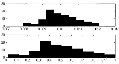
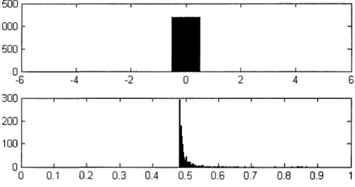
4.5 PageRank versus in-degree for T2(4). 69 4.6 PageRank versus in-degree distributions for the

binary tree T2 (4). 70

4.7 The general form of a binary tree with the labeled nodes. Here xr^ denotes the i-th node on the r-th

row. 72 4.8 The location of some of the nodes used in the

viii LIST OF FIGURES

4.9 PageRank versus in-degree in a random digraph

with 100 nodes. 78

4.10 PageRank versus in-degree in a power law digraph

CHAPTER 1

Introduction 1.1. M o t i v a t i o n

With the rapid growth of the world wide web, informa-tion retrieval presents increasing theoretical and practical challenges. With the massive amount of information enter-ing the world wide web every moment, it becomes harder and harder to retrieve information from the web. That is why the presence of a search engine is as vital as the exis-tence of the web itself. Since the birth of the web, it has been a central discussion in the web research community to design faster, more efficient, and more accurate search engines.

The most popular search engine currently is Google. The mathematical theory behind the Google search engine is the PageRank algorithm, which was introduced by Sergey

B r i n a n d L a w r e n c e P a g e [3], t h e f o u n d e r s of G o o g l e . I n

1998, Brin and Page were PhD students. They took a leave of absence from their Ph.D. to focus on developing their

2 1. INTRODUCTION

Google prototype. Their pioneering paper described the PageRank algorithm, which is used to this day by Google to generate its rankings.

A search engine consists of key components: a crawler, and indexer, and a query engine [2]. The crawler collects and stores data from the web. Data is stored in an indexer which extracts information from the data collected from the crawler. The query engine responds to queries from users. As part of the query engine, a ranking algorithm, ranks web pages in order of their relevance to the query. The ranking is achieved by the assignment of a score to each web page. PageRank is a ranking algorithm of web pages and uses the link structure of the web. The web's link structure forms a directed graph where the web pages are represented as nodes and links as directed edges. A page is considered "important" if it is pointed to by other important pages. The following PageRank equation finds a score by solving the iterative equation:

1.1. MOTIVATION 3

where J is the matrix of all l's whose order equals the number of pages. The matrix S is the stochastic matrix as-sociated to the directed adjacency matrix of the web graph. The parameter a is called the teleportation factor, a con-stant between 0 and 1 which is normally assumed to be around 0.85, and TT is the PageRank vector [13]. PageRank will be discussed in detail in Chapter 2.

The PageRank vector consisting of the PageRank of each web page is the stationary value of a large ergo die Markov Chain [3]. The Perron-Frobenius theorem is used to en-sure that the so-called Google matrix associated with this Markov Chain will converge to a stationary distribution

[15]. The Perron-Frobenius theorem supplies a unique nor-malized positive dominant eigenvector, called the Perron

Vector, which is the PageRank vector of the Google

ma-trix.

In a recent work by Litvak, Scheinhardt, and Volkovich [14], a mathematical model is presented that derives an interest-ing relation between PageRank values and in-degrees of web pages. They investigate why the PageRank and in-degree of

4 1. INTRODUCTION

web pages follow similar power laws in the web graph. Fur-thermore, they analytically prove that in power law graphs, the tail distributions of PageRank and in-degree differ only by a multiplicative factor [14].

The aim of my thesis is to first survey the mathematics of the PageRank algorithm, and then to investigate the recent work of [14]. In Chapter 2, I introduce PageRank and describe its key properties. I will implement a PageRank calculator and expose different graphs to my calculator. In Chapter 3, we summarize the work of [14], who proved t h a t the ranking of the nodes by PageRank in power law graphs will be similar to their ranking via their in-degree values. For binary trees, we show in Chapter 4 that the ranking result from PageRank is different from the ranking of their in-degree values.

What follows in this chapter is the background and def-initions needed throughout my thesis. As we will see, the mathematical study PageRank uses a blend of graph the-ory, probability, and linear algebra.

1.2. GRAPH THEORY 5

1.2. Graph T h e o r y

This section gives a concise introduction to the graph theory terminology used later in my thesis. For a general reference in graph theory, see [6]. A graph G consists of a nonempty vertex set V(G), and an edge set E(G) of 2-element subsets from V(G). A graph is sometimes called

network, especially with regards to real-world examples.

More formally, we may consider E(G) as a binary rela-tion onV(G) which is irreflexive and symmetric. We often write G = (V(G), E(G)), or if G is clear from context, then we write G = (V, E). The set E may be empty. Elements of V are vertices, and elements of E are edges. Vertices are occasionally referred to as nodes, while edges are referred to as lines or links. We write uv for an edge {u,v}, and say that u and v are joined or adjacent; we may as well say that u and v are incident to the edge uv, and that u and

v are endpoints of uv. The most common way to visualize

a graph is by drawing a dot for each node and joining two of these dots by a line if the corresponding two nodes form an edge. By a non-empty graph, we mean a graph with at least one edge.

6 1. INTRODUCTION

We allow graphs to have multiple edges, but no loops. A simple graph is a graph without multiple edges. The cardinality |V(G)| is the order of G, while |£?(G)| is its

size. For a node v G V(G), degc{v) is the degree of v in G,

namely the number of edges in G incident with v. A node of degree 0 is isolated.

For a node re in a graph G, define the neighbourhood of x, written NQ(X), to the nodes joined to x. For X C V(G),

NQ{X) is the union of the neighborhoods over nodes from X. If X C V, then define the subgraph induced by X,

written G \ X (or as either (X)G or G*[X]), to be the graph with nodes from X, with two nodes joined in G \ X if and only if they are joined in G. A subgraph of G is a graph H such that V(H) C V(G) and E(H) C E(G). A graph G is called bipartite if V(G) admits a partition into two classes such that every edge has its ends in different classes (hence, nodes in the same partition class must not be adjacent).

A graph may be directed or undirected. A directed graph or digraph is defined analogously as an undirected graph, except that now E{G) need not be a symmetric binary relation on V(G). The edges are written as ordered pairs,

1.2. GRAPH THEORY 7

and are called directed edges, (u,v), where u is the head and v is the £ai/. The directed edge (u, v) is then said to be directed from u to v. All the previously mentioned features and definitions can then be modified to directed graphs. The in-degree of u, written deg~(u), is the number of nodes v such that (v, u) are directed edges; the out-degree deg+(w) is defined dually. Moreover, a directed graph is

called strongly connected if for each pair of nodes (vi,Vj), there is a sequence of directed edges leading from Vi to Vj. The directed graph in Figure 1.1 is strongly connected. In

FIGURE 1.1. A strongly connected digraph.

all of the above definitions, we will not mention G if it is clear from the content.

One of the most important examples of a graph for us is the web graph. It is the graph where the nodes represent web pages, and the edges correspond to links between the

8 1. INTRODUCTION

pages. We write W for this graph, which is a real-world evolving graph. We may consider W an undirected or di-rected graph, depending on the context.

A key property of the web graph is the presence of a power-law degree distributions. Given a graph G and a non-negative integer fc, we define NkjG by

Nk,G=\{xeV(G):degG(x) = k}\.

The parameter Nk,G is number of nodes of degree k in G.

The degree distribution of G is the sequence (N^^G '• 0 <

k <t). The degree distribution of G follows a power law if

for each degree k,

Nk,G h_p

—— ~ k p,

t

for a fixed real constant j3 > 1. We say that (3 is the

ex-ponent of the power law. A graph whose degree

distribu-tion follows a power law is often referred to as a power law

graph. Power laws for the in-degree and out-degree

distri-butions may be defined in a similar fashion. The in- and out-degree distributions of the web graph were observed to follow power law in the experiments conducted by Broder

1.3. LINEAR ALGEBRA 9

et al. [4], which sampled 200 million web pages and their links. For additional reading on the web graph, the reader is directed to the books [2, 5, 8].

1.3. Linear Algebra

Matrices and vectors will be denoted in bold. Further, all vectors are column vectors unless otherwise stated. For a matrix A, we use the notation a^ for the zj-entry of A. An m x n matrix A is a non-negative matrix whenever each a,ij > 0, and this is denoted by writing A > 0. The notation A > B means that each a^ > bij. A matrix A is

positive when each a^ > 0, and this is denoted by writing

A > 0. More generally, A > B means that each a^- > b^. A convenient representation of a graph is via its adja-cency matrix. The adjaadja-cency 'matrix A(G) of a digraph G is defined by

( 1 i f ^ - e E ( G 9 ,

aij = <

I 0 otherwise.

If G is undirected of order n, then A(G) is an n x n symmet-ric (that is, A(G) = A(G)T) matrix. Adjacency matrices

10 1. INTRODUCTION

For an n x n matrix A, a scalar A for which

det(A - AI) = 0

is called an eigenvalue of A. A nonzero n x 1 vector x for which A — Ax is the eigenvector of A for A. The pair (A,x) is called an eigenpair for A. The set of all distinct eigenvalues, denoted by <J(A) , is called the spectrum, of A.

The eigenvalues and eigenvectors are fundamental topics in PageRank calculations. The adjacency matrix A(G) for an undirected graph G is a real and symmetric matrix, and hence, has n real eigenvalues Ai > 0, A 2 , . . . , An, which can

be ordered by their absolute values:

Ai = |Ai| > |A2| > . . . > |A„|.

(See, for example, [2].) The first (that is, largest in absolute value) eigenvalue Ai is the radius of the spectrum, denoted by p(A). The real number Ai is also called the dominant

eigenvalue.

We now state Perron-Frobenius theorem. A proof of this important result may be found in [15]. A non-negative matrix A is primitive if Am > 0 for some m > 0. The

1.3. LINEAR ALGEBRA 11

1-norm (or taxicab norm) of x is defined as

Mli = £

n T • I

•1=1

THEOREM 1.3.1 (Perron-Frobenius). If a matrix A > 0

is primitive, then each of the following assertions holds.

(1) r = p(A) > 0.

(2) There exists an eigenvector x > 0 such that A x = r x .

(3) The Perron vector p is the unique vector satisfying

Ap = rp

and which is positive with 1-norm equal to 1. There are no other non-negative eigenvectors for A regard-less of the eigenvalue, except for the positive multi-ples of p.

We will sometimes use limits of matrices. If (Mt) is a

sequence o f m x n matrices, and L is an m x n matrix, then we write

lim Mt = L

12 1. INTRODUCTION

if for all 1 < i < m, 1 < j < n,

lim {Mt\3 = Lid.

t—>oo ,J

1.4. Markov Chains

Markov Chains provide a powerful framework for mod-elling certain random processes. Our approach to ana-lyze the PageRank algorithm in Chapter 2 will use Markov chains. We give a brief discussion of Markov chains in this section. For a general reference in probability theory, see

[11].

Fix n a positive integer. We denote ¥(A) the probability of an event A in a probability space. A (discrete-time,

time-homogeneous, finite-state) Markov chain M consists

of a discrete-time random process (Xt : t G N) each with

codomain in the same finite set S — { a o , . . . ,an} with the

property that for all n > 1 and 1 < t < n,

<H-i)-1.4. MARKOV CHAINS 13

This definition expresses that the state Xt depends on the

previous state Xt-i, but is independent of how we actu-ally arrived at Xt~\. In other words, the random process does not remember the way it reached the state Xt-\. This

property is called Markovian or memoryless property for a random process. It is important to note that the Markov property does not imply that the state Xt does not depend

on the random variables XQ, X\,..., Xt-2- However, what a

Markovian property guarantees for Xt, is that any such de-pendency on the past will be captured and recorded in the value of Xt-\. In other words, only the present state giyes any information of the future behaviour of the process. See

[16] for more background on Markov chains.

The set of possible values S of M is called the state

space, and without loss of generality we will always consider

this to be { 1 , . . . , n}, where n is an integer. The transition

probability

P

=F(X

=j\X

-i=i)

is the probability that the process moves from state i to state j in one time-step. Using the Markovian property,

14 1. INTRODUCTION

every Markov chain can be uniquely expressed by a

transi-tion matrix defined as

/ P = Po,o Po,i Plfi P\,l Pifi Pi,I

p

V

Hence, the zj-entry in the matrix is the transition prob-ability Pi j . The representation of a Markov chain via its transition matrix makes it feasible to compute and predict the distribution of the future states of the process.

A useful representation of a Markov chain is via a di-rected weighted graph. The nodes correspond to the states, and the weight on each directed edge is the positive transi-tion probability of getting from the head state to tail state. There is a directed edge (i,j) if and only if Pij > 0. A

sto-chastic matrix is a non-negative matrix in which each row

sum is equal to 1. Note that the transition matrix of every Markov chain is a stochastic matrix (which follows from the basic probability definitions). A stationary distribution

1.4. MARKOV CHAINS 15

s of a Markov chain is a probability distribution (that is, a vector whose sum of all entries equals 1) with the property that

sT = sTP .

We can also express this by saying that s is an eigenvector of P with eigenvalue 1, or s is a fixed-point of P .

Stationary distributions exist and are unique if the Markov chain has a primitive transition matrix [2]. We refer to such Markov chains as ergodic. Hence, if we consider an ergodic Markov chain over a long period of time, the initial state becomes increasingly forgotten, and the probability that we are in state i approaches the ith component of s. As we will see in Chapter 2, the PageRank vector corresponds to the stationary distribution of a certain Markov chain.

CHAPTER 2

T h e P a g e R a n k A l g o r i t h m 2.1. Introduction and M o t i v a t i o n

Information retrieval is the process of searching within a collection of documents for a particular item of information. The information you are looking for is normally called a

query. To retrieve information from the world wide web,

we need to first be able to model the web. The best way to model a massive network like the web is by representing it as a digraph. Each web page is a node of the graph and the links between two nodes are directed edges. To perform a search in this network, we should first be able to gather all of the information about its link structure in a database, and then classify and retrieve the query from this database. A search engine consists of a crawler, indexer and a

query engine; see [13]. See Figure 2.1 for a simplified model

of a search engine.

18 2. THE PAGERANK ALGORITHM

Crawler Indexer Query Processor

' •

Ranking of the Results

F I G U R E 2 . 1 . A basic search engine model.

The crawler performs frequent visits to t h e entire (or a large part of the) world wide web. The crawler trav-els from page to page to keep track of the existing links, and more importantly to update our database with new web pages and links. Imagine a backpacker who is walking through every link, and upon arriving at every new web page, writes down the address of the page and summarizes its content. There are certainly web pages that have no out-links. Hence, our backpacker will get stuck there. Af-ter recording such pages (called dangling nodes), the back-packer will step back as many steps needed to be able to find a way out.

The links are classified once they are entered into t h e indexer. Hence, now we can search for our query in t h e

2.2. RANDOM WALKS ON GRAPHS 19

indexer. The search is done, and some number of pages associated to the query are found.

After the search is done, let us say there are 200 pages found in the end. The question becomes: how to rank these pages? A useful way to display the 200 pages on the result screen is to rank them by popularity. We therefore need to find out how to rank web pages according to their popularity. This is the role of the query engine. As we will describe in Section 2.2, the PageRank algorithm is one effective way to accomplish this ranking.

2.2. R a n d o m Walks on Graphs

Before we define PageRank, we make a short digression to discuss random walks. A random, walk on a connected graph G is a certain type of Markov chain defined by the sequence of moves (over discrete time-steps) of a particle between nodes of G. The location of the particle at a given time-step is its state. In the uniform random walk, the par-ticle may move from its current state to any of its neigh-bouring nodes (with equal probability). A uniform random walk on a graph of size n may be represented by a transition

20 2. T H E P A G E R A N K A L G O R I T H M

probability matrix P whose entries are p^-, where

Pij = <

I 0 otherwise.

Note that the transition probability matrix of a uni-form random walk is stochastic; that is, the row sums are equal to 1. We define an ergodic Markov chain to be one whose transition matrix is primitive. An important the-orem states that an ergodic Markov chain always has a stationary distribution [19]. Hence, the stationary proba-bility distribution exists for the uniform random walk if its transition matrix is primitive, and is a probability vector sT such that

sTP = sT.

The following theorem states sufficient conditions on G for the stationary distribution to exist.

T H E O R E M 2.2.1. [2] Let G be a finite, connected,

non-bipartite graph. A random walk on G converges to a sta-tionary distribution sT = (SJ), where

_ deg(i) S%~2\E(G)[

2.3. THE GOOGLE MATRIX 21

Analogous result holds for uniform random walks on di-rected graphs.

2.3. T h e Google M a t r i x

To define the Google matrix for an arbitrary graph G, we consider the transition probability matrix for the uniform random walk on G. Let n = \V(G)\ be the order of G and apply a fixed enumeration from 1 to n to the nodes of G. For the directed graph G, the matrix P i is defined by

I 0 otherwise.

The structure of the P i matrix guarantees that at every node, the surfer will have equal probability to choose one of the out-neighbours. If there is no out-link from i to j , then this probability is 0. In the web there always exist web pages that do not link to any other web pages. These nodes are called dangling nodes. If we assume the only way to visit the web pages is by following the out-links, then the surfer gets stuck at such nodes. To overcome this problem, we manipulate the matrix P i in a way to bypass the dangling nodes. Define P2 to be the matrix P i such

22 2. T H E P A G E R A N K A L G O R I T H M

that any zero rows are replaced with the vector with each entry equal to - . Define the Google matrix (or PageRank matrix) by

1 — a

P = a P2 H J„,n,

n

where a; is a fixed real number in (0,1), and Jn j n is the nxn

matrix of all l's. (We do not use the notation G for the Google matrix, as G is reserved for graphs.) The constant

a, called the teleportation factor, is a parameter measuring

the frequency at which a surfer jumps to a new randomly chosen web page, rather than following the out-links. We now show why Google matrix is stochastic and primitive, and hence, has a stationary distribution.

LEMMA 2.3.1. For a graph G with order n and P = P(G*) equalling its Google matrix, then the following

asser-tions hold.

(1) The matrix P is stochastic. (2) The matrix P is primitive.

Proof. For item (1), to show that P is stochastic, we

2.3. THE GOOGLE MATRIX 23

a fixed 0 < i < n, the row sum r,b equals:

Ti = ^ ( a (P2 k j + — ^ — (Jn,n)ij)

Kj<n ^ '

1 — a

= " E (P2)*J + ( ! - « ) •

l < j < n

To find the value for J^ (^2)1^, we consider two cases. Case i. Node i is dangling node.

In this case,

(P

)„ = i.

= a V - + (1 -

a)

Case £. Node i is not dangling. In this case,

24 2. T H E P A G E R A N K A L G O R I T H M

Hence,

n = a J2 (Pikj + ( l - a )

l<j<n

— a + (1 — a) = 1.

For item (2), since all entries of P are positive, P is primi-tive. •

Lemma 2.3.1 demonstrates that the Google matrix P is a transition probability matrix of an ergodic Markov chain. The Markov chain associated to this matrix is called the

PageRank Markov chain, or the PageRank random, walk.

In this random walk, at any page, the surfer visits an out-neighbour of that node with probability a and visits any other node in G with probability 1 — a. In practice, the parameter a is normally assumed to be around 0.85; see

[13].

We will now use the linear algebra preliminaries stated in Chapter 1 of the thesis to prove an important theorem about the PageRank random walk. The following theorem

2.3. THE GOOGLE MATRIX 25

guarantees that with the described structure of Google ma-trix, the PageRank random walk has a unique stationary distribution, called the PageRank vector.

THEOREM 2.3.2. Fix a graph G. The PageRank Markov

chain with transition probability matrix P = P ( G ) con-verges to a unique stationary distribution s.

Proof. Since P is positive and primitive, the PageRank

Markov chain is ergodic, and hence, converges to a station-ary distribution s. To show that s is unique, we will use the Perron-Frobenius theorem (See Theorem 1.3.1). By Theo-rem 1.3.1, P has a unique positive and dominant eigenvalue equal to 1. The corresponding eigenvector for this eigen-value would be the vector s, where

s

P = s

. •

The vector s is the PageRank vector for the Google ma-trix P . The entries in the PageRank vector are the PageR-ank values for each node in the graph G (associated with the fixed enumeration of V(G)). To calculate the PageRank values, we need to find the stationary vector of the Google

26 2. T H E P A G E R A N K A L G O R I T H M

matrix. In Section 2.4 we discuss a practical method used to calculate the PageRank, called the power method. In the next section, we explain another approach to calculate the PageRank vector first used by Brin and Page [3].

2.4. A n o t h e r V i e w of P a g e R a n k

The original formula for PageRank due to [3], is a sum-mation formula which calculates the popularity of the pages by adding up the PageRank of all the pages pointing to this web page. Let PR(Pi) denote the PageRank of the page

Pi and let In(Pi) denote the set of web pages that point to Pi. The PageRank is then

(2.i) PR(P,)= J2

^§r-A problem is that the values for PR(Pj) are unknown. To overcome this, we need to initialize all the web pages with an equal PageRank value, and then transform equation (2.1) into a recursive equation. Brin and Page assumed that at the beginning all the pages have a constant PageR-ank value of - , where n is the total number of pages in the web graph. The iterative procedure calculates PageRank

2.5. THE WORLD'S LARGEST MATRIX COMPUTATION 27

at (k + l)-th step as

(2.2) PRM(P,)= £ ^ p .

The process initiates with setting PRo(Pi) — ^ for all pages

Pi. As discussed in the previous section, since the

PageR-ank Markov chain is ergodic, the eventual convergence of the PageRank scores is guaranteed.

2.5. T h e World's Largest M a t r i x C o m p u t a t i o n

Cleve Moler, the founder of the well-known mathemati-cal software matlab, cited PageRank as "The World's Largest Matrix Computation" in [17]. At that time Google was ap-plying the Power Method to a sparse matrix of order 2.7 billion. Now, it has at least 54 billion rows and columns!

(See [2].)

To find the PageRank vector, we should solve for the eigenvector s such that

sTP = sT.

Since P is a dense massive matrix, a direct approach to the calculations will not be feasible in general. To overcome

28 2. T H E P A G E R A N K A L G O R I T H M

the computational problems, the power method is used to approximate the PageRank vector s. The algorithm works as follows. Fix a directed graph G of order n.

(1) Initialize zo to be the stochastic vector with every entry equal to 1/n.

(2) Define

z

= zpP = (zj )P*

The sequence (z& : k € N) consists of stochastic vectors, since at every time step, we have the result of the product of two stochastic matrices. It can be shown that

Inn zfc+i

K—>00

is the dominant eigenvector of the Google matrix; see [2]. From the Power method, we can approximate the PageR-ank vector by taking powers of the Google matrix and mul-tiplying it by zo- This amounts to simply summing up each column of P and multiplying the sum by 1/n.

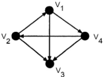
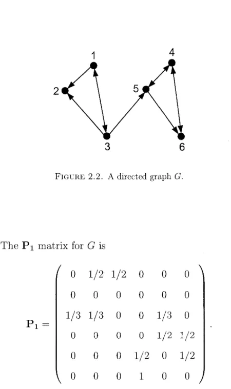
For completeness, we give an illustration of a PageRank computation. Figure 2.5 shows a sample graph G with six nodes. To find the PageRank vector of G. we first compute

2.5. THE WORLD'S LARGEST MATRIX COMPUTATION 29

the various matrices required in the definition of the Google matrix.

FIGURE 2.2. A directed graph G.

The P i matrix for G is

Pi \

(

0 1/2 1/2 0 0 0

0 0 0 0 0 0

1/3 1/3 0 0 1/3 0

0 0 0 0 1/2 1/2

0 0 0 1/2 0 1/2

\ 0 0 0 1 0 0

j

30 2. THE PAGERANK ALGORITHM The P2 matrix is ( 0 1/2 1/2 0 0 0 \ 1/6 1/6 1/6 1/6 1/6 1/6 1/3 1/3 0 0 1/3 0 0 0 0 0 1/2 1/2 0 0 0 1/2 0 1/2 \ 0 0 0 1 0 0 /

If a = 0.85, then let a = a / 2 , b = (1 — a ) / 6 , c = a / 6 , and

d = a / 3 . Then the Google matrix of G is then

1 b a + b a + b b b b ^

6 + c 6 + c 6 + c 6 + c 6 + c

b + c

b b b b

a + 6 0 + 6

Using the power method, the approximate PageRank vector (using the natural ordering {1,2,3,4, 5,6}, and with two decimal places of accuracy) is

2.6. IMPLEMENTATION OF A PAGERANK CALCULATOR 31

2.6. I m p l e m e n t a t i o n of a P a g e R a n k Calculator

In this section, a brief description of an implementa-tion of PageRank is given on a graph with n nodes. The PageRank calculator implemented for the thesis uses the algorithm provided in [13].

(1) The vector piO is the initial vector, which we nor-mally set to 1/n.

(2) H is the manipulated hyperlink matrix, P%. (3) n is the size of the matrix or the web. (4) a l p h a is the teleportation factor.

(5) e p s i l o n is the convergence tolerance; in the ac-tual implementation, we set the total iteration steps equal to 20.

(6) The vector a is the dangling node vector in which an entry is 1 if its corresponding node is a dangling node, and 0, otherwise.

%Implementation of PageRank c a l c u l a t o r %using power method

f u n c t i o n [ p i , t i m e , n u m i t e r ] =

32 2. T H E P A G E R A N K A L G O R I T H M rowsumvector=ones(l,n)*H'; nonzerorows=find(rowsumvector); zerorows=setdiff(1:n,nonzerorows); l=length(zerorows); a=sparse(zerorows,ones(l,1),ones(l,1),n,1); k=0; residual=l; pi=piO; tic; for ( i=0:20 ) %while(residual < epsilon) prevpi=pi; k=k+l; pi=alpha*pi*H + (alpha*(pi*a)+l-alpha) *((l/n)*ones(l,n)); r e s i d u a l = n o r m ( p i - p r e v p i , 1 ) ; end; numiter=k; t i m e = t o c ; 70save p i ;

CHAPTER 3

P a g e R a n k in Power Law Graphs

PageRank roughly measures the popularity of a web page based on its number of in-links. We discussed PageR-ank in detail in Chapter 2, and we proved that it is the stationary distribution of the PageRank random walk. We now present recent work by Litvak et al. [14], who proved that under certain assumptions PageRank and in-degree distributions of a power law digraph obey a power law with the same exponent. To prove this result, we model the re-lation between PageRank and in-degree via a stochastic equation. All the results described in this chapter come from [14].

Studying the potential similarity between PageRank and in-degree of the web pages is of particular importance be-cause it provides ground for simpler, cheaper and less time-consuming calculations. The matrix calculations performed to estimate PageRank, are massive. However, it is straight forward to find the in-degree of a web page.

34 3. PAGERANK IN POWER LAW GRAPHS

To study the behaviour of the PageRank tail, Laplace-Stieltjes transforms are used. The Tauberian Theorem and the theory of regularly varying variables are then applied to a certain stochastic equation to prove analytically t h a t the tails of PageRank and in-degree distributions vary only in a multiplicative constant. Hence, the PageRank and in-degree distributions in power law graphs follow power laws with the same exponent.

We begin by recalling the PageRank equation in its sum-mation form. (See Equation 2.1 from the previous chapter.)

(3.1) PR(i) =

a J2 ^ T ^ + (1 - ")•

jeN(i) J

An interpretation of (3.1) is that the PageRank of node

i depends on the degree of i and PageRank of its

in-neighbours. However, it is important to note that while the linear algebraic methods often used in PageRank lit-erature work well for most PageRank computations, they are not sufficient for analyzing the asymptotic properties of the PageRank distribution. The mathematical approach to PageRank analysis used in [14] stems more from applied

3. PAGERANK IN POWER LAW GRAPHS 35

probability and stochastic operations research, than from linear algebra.

In Donato et al. [7], Fortunato et al. [9] and Becchetti and Castillo [1], experiments performed on the web graph confirm the similarity in tail behavior of PageRank and in-degree distributions. The exponent value (3 for the power laws of the PageRank and in-degree distributions were found in all cases to be around 1.1. Moreover, the cited experi-mental studies have shown that the PageRank of the top 10% of the nodes always follows a power law with the same exponent independent of the teleportation factor a.

In a power law distribution, there is a so-called 30-70 rule: the tail will cover 70 percent of the value of the distri-bution. We will therefore compare the tail distribution of PageRank and in-degree. In other words, we focus on tail

asymptotics for PageRank and its relation with in-degree.

Since we are only interested in the tail, we are looking into web pages with high popularity or PageRank value, which can be stated as

36 3. PAGERANK IN POWER LAW GRAPHS

for a suitably large x, and where F(A) is the probability of the event A in a probability space. Observe that (3.2) defines the fraction of pages having PageRank greater than

x, where x is large. One way to analyze such a probability

is to find an asymptotic expression p{x) for which ,. F(PR > x) .,

lim — — — — - = 1. x^oo pyx)

If such a p(x) is found, then p(x) and ¥(PR > x) are asymptotically equal, and so we can approximate the tail of PageRank by p(x).

3.1. Regularly Varying R a n d o m Variables

A real-valued function RV(x) is said to be regularly

varying of index j3 G M. if for every t > 0,

lim ™ =

if.

z-»oo RV(X)

A real-valued function SV(x) is said to be slowly varying

if for every t > 0,

SV{tx) l i m "cTTTT = x

-3.1. REGULARLY VARYING RANDOM VARIABLES 37

A careful look at the above definitions leads us to a relation between RV and SV functions: every regularly varying function can be written as

RV(x)=x<3SV{x),

for some slowly varying function. We can also define the

regularly varying property for random variables as well as

functions. Recall that a(x) ~ b(x) if

a(x)

l i m T^T = L

A random variable X is said to be regularly varying with

index (3 if its distribution F(x) can be written as

1 - F ( x ) ~ x~pSV{x),

for some slowly varying function SV(x). The

Laplace-Stieltjes transform of X is

38 3. P A G E R A N K IN P O W E R L A W G R A P H S

where s > 0 and E(Y) is the expectation of the random variable Y. The n-th moment of X is written as

poo

£„ = / XndF(x).

Jo

By expanding / in a series at s = 0, the successive moments of F can be obtained. Moreover, the n-th moment of X is finite if and only if there exist coefficients £0, • • •, £,n such

that fn(s) — o(sn), as s —» 0. The following lemma states

this in a precise fashion.

LEMMA 3.1.1 ([14]). The n-th moment of X is finite if

and only if there exist real numbers £0 = 1 and £i> • • • > £n; such that

n p

s—>0 •«•—' ? !

i=0

The above coefficients & may be uniquely found. If £n <

co, then we write:

fn(s) = (-ir

+i

(f(s)-J2^(-

s

^

\ i=0

Later, we will use fn(s) further to discuss the tail

3.2. THE RELATIONSHIP BETWEEN IN-DEGREE AND PAGERANK 39

between asymptotic behaviour of a regularly varying distri-bution and its Laplace-Stieltjes transform. The following theorem, used throughout this chapter, makes this relation precise.

THEOREM 3.1.2 (Tauberian Theorem; [14]). For n G N

and if£n < oo7 (3 = n + r), and rj G (0,1), then the following are equivalent

(1) /n( s ) ~ ( - 1 ) ^ ( 1 - pySV{% ass^O

(2) 1 - F(x) ~ x-PSV(x), as x -> oo.

The proofs of the above lemma and theorem may be found in [14]. Theorem 3.1.2 plays an important role in finding the relation between asymptotic distributions of PageRank and in-degree.

3.2. T h e Relationship b e t w e e n In-degree and P a g e R a n k

We now describe the relationship between PageRank and in-degree. We consider equation (3.1), but make some important simplifying assumptions. These assumptions will enable us to model this relation by focusing on the influence of in-degree without considering other factors. Naturally,

40 3. PAGERANK IN POWER LAW GRAPHS

these assumptions are not realistic, but in further discus-sions we try to reduce them by generalizing the model ob-tained. Rewrite equation (3.1) in the following form of a distributional identity with the random variable R:

M

(3.3) R = a^2-Rj + (l-a),

Lb

3=1

where = represents a distributional identity and M is the in-degree of the considered random page. The assumptions we make are as follows.

(1) Let R represent the PageRank of a randomly chosen page. One of our goals in this chapter is to deter-mine the distribution of the random variable R. (2) Fix d > 1 and assume that it is the number of

out-going links for all pages. Hence, out-degree is equal for all nodes.

(3) The dangling node effect is neglected. That is, we do not consider the effect of pages without outgoing links.

(4) The random variables R and M are independent. That is, the in-degree distribution and PageRank

3.2. THE RELATIONSHIP BETWEEN IN-DEGREE AND PAGERANK 41

distribution of a random page have independent dis-tributions (which is not the case, in general). (5) All Rj's are independent and have the same

distri-bution as R and hence, R = 1 constitutes the unique solution of the equation (3.3).

The equation (3.3) has the same form as the original PageR-ank formula as in equation (3.1).

We will now find the in-degree distribution for a ran-domly chosen web page. Although it is well-known that the in-degree distribution of the web graph follows power law (see for example, [2]), we need to be able to formally describe this random variable for our analysis. We use the theory of regularly varying random variables. The in-degree of a randomly chosen page is modeled by a non-negative integer-valued, regularly varying random variable which is distributed as N(X). In particular, the random variable X is regularly varying with index (3 and N{x) is the number

of Poisson arrivals on the time interval [0, x\. For more

de-tails on Poisson processes and their application in Markov chains, see Sections 8.2 and 8.3 of [12].

42 3. PAGERANK IN POWER LAW GRAPHS

The variable N(x) is a "discretization" of the random variable X. In this way, we guarantee that while in-degree has a power law distribution, it only takes integer values and hence, we do not have to put any restrictions on X. In Theorem 3.2.1 below, we will prove that N(X) is also regularly varying with the same index as X , and so fol-lows a power law with the same exponent. First, let Fx and FN(X) be the distribution functions of X and N(X), respectively. Let / and <fi be their corresponding Laplace-Stieltjes transforms.

THEOREM 3.2.1 ([14]). The following are equivalent. (1) 1 - Fx(x) ~ x-PSV(x), as x -> oo

(2) 1 — F/v(x) ~ x~^SV(x), as x —> oo

We give a brief sketch of the theorem. We first need a technical lemma.

L E M M A 3.2.2 ([14]). Let fn(s) and(j)n(s) be the Laplace-Stieltjes transforms of X and N(X), respectively. Then

3.2. THE RELATIONSHIP BETWEEN IN-DEGREE AND PAGERANK 43

While we omit the proof of the lemma, here is an infor-mal sketch of its proof. One shows that the corresponding moments of X and N(X) always exist. It may be shown that since we fixed the out-degree of all pages to be equal to d, then the average in-degree would also equal d. That is, E[X] = d and similarly, E[N(X)] = d. The final step in the proof of Lemma 3.2.2 is to consider the generating function of N(X) and derive its Laplace-Stieltjes transform in terms of the Laplace-Stieltjes transform of the random variable X.

We now sketch a proof of Theorem 3.2.1.

P r o o f of T h e o r e m 3.2.1. We only prove that (1)

implies (2). Prom Theorem 3.1.2 in the previous section, we have that

1 — Fx{x) ~ x~^SV(x), as x —> oo

implies that

fn(t) ~ ( - 1 ) ^ ( 1 - 0)1?SV Q , as t -* 0

where n is the largest integer smaller than /?, and T is the

44 3. PAGERANK IN POWER LAW GRAPHS

have that fn(s) ~ o(sn) where t(s) = 1 — e~s ~ s. By

Lemma 3.1.1 and Theorem 3.1.2, we have that

1 — FN(X)(X) ~ x_ / ?5F(a:) as x —> oo. D

The model of Litvak et al. for the number of incoming links of a randomly chosen web page works well, since it de-scribes an in-degree distribution which follows a power law with finite expectation and a non-integer exponent (3 > 1. Having obtained the distribution for in-degree and PageR-ank, we will now proceed to retrieve the main stochastic equation for the relation between PageRank and in-degree and compare their tail distributions in the next section.

3.3. Stochastic Equations

Using the discussion in the previous two sections, we can now reformulate the equation (3.3) as follows:

N(X)

(3.4) R = a Y; -jRj + {l-a),

CX 3 = 1

where a € (0,1) is the teleportation factor, d > 1 is the fixed out-degree of each page, and N(X) describes the in-degree of a randomly chosen page in terms of the Poisson

3.3. STOCHASTIC EQUATIONS 45

arrivals on a regularly varying random variable X which represents time. The stochastic equation (3.4) adequately represents the PageRank distribution and its relation with the in-degree distribution. We can now apply analytical methods to study the tail behaviour.

The main idea of the analysis is to apply the Laplace-Stieltjes transforms of X and R. By using the Tauberian Theorem, we may prove that R is regularly varying with the same index as X. By the Theorem 3.2.1, this then guarantees similarity in the tail behaviour of the PageRank

R and the in-degree N{X).

The first step is to write the Laplace-Stieltjes transform of the PageRank distribution R in terms of the probability generating function of N(X). Let GN(X) be the generating function of N(X). By applying Laplace-Stieltjes transform

46 3. PAGERANK IN POWER LAW GRAPHS

to the definition of R in (3.4) we have that

r{s) = E[e-sR] = E{e-<l-a^}E a

~d N{X)

exp | — s— \] Ri

exp

r4E^

F(N(X) = k)

r\s-X) F{N(X) =k)

Note that for all i, we have Ri = R, and that is how the second equality in the above set of equations is obtained. In the following corollary, we prove that GJV(X) c a n be

ex-pressed in terms of the Laplace-Stieltjes transform of X.

COROLLARY 3.3.1 ([14]). I/GN(X) ^ the generating func-tion of N(X) and f is the Laplace-Stieltjes transform of X, then we have that

3.3. STOCHASTIC EQUATIONS 47

Proof. By definition of the generating function,

GN(X)(S) = E[sNW] roo

= / E[s

®]dFx(t)

Jo

The above corollary leads us to an important conclusion for the Laplace-Stieltjes transform of R. By Corollary 3.3.1, as

CJV(X)(S) = / ( I — s) w e obtain that

(3.5) r(s) = f(l-r(^s))e-<1-a\

As in the previous section where the distribution for in-degree was calculated, here we perform the analysis by showing the correspondence between the existence of the n-th moments of X and R. The independence of N(X) and the Rj's is heavily used. For example, using this in-dependence, we can take the expectation from both sides

48 3. PAGERANK IN POWER LAW GRAPHS

of (3.4). Similar to the result of Lemma 3.1.1, we can re-formulate it and show that

(3.6) fn(s) = o{sn) if and only if rn{s) = o(sn).

Now we can present the final theorem in this chapter in which the observed correlation between in-degree and PageR-ank distributions is explained in power law graphs. The proof of the theorem can be found in [14].

THEOREM 3.3.2. The following are equivalent.

(1) 1 — FN(X){X) ~ x~^SV(x), as x —> oo In particular,

N(X) is a regularly varying random variable with index j3.

(2) 1 — FR{X) ~ d0<^a/3dx~f3SV(x), as x —> oo. In partic-ular, R is a regularly varying random variable with the same index (3.

Theorem 3.3.2 shows that the asymptotic behaviour of PageRank and in-degree are similar in power law graphs, since they both follow a power law with equal exponents (they differ only by the multiplicative factor J^_ Pd).

3.4. NUMERICAL EXPERIMENTS AND CONCLUSION 49

3.4. Numerical E x p e r i m e n t s and Conclusion

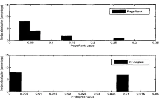
How do we verify a power law behaviour in practice? It is not always simple to plot, measure, or numerically identify power law distributions. A well-known technique is to plot the so-called log-log graph of the distribution. More precisely, we plot the degree distribution in logarith-mic scale and expect to obtain a straight line. Experiments conducted by Newman in [18] suggests that since we are focusing on tail distributions, we should plot the fraction of quantities which are not less than a certain value. In particular, we should plot the complementary cumulative function instead; that is,

l-F(x)=F(X >x),

rather than to plot the histogram. In this way, we will have a more concentrated plot.

Another issue is that if a distribution X follows power law with exponent (3 such that 1 — F(x) ~ Cx~^, where C is a constant, then the corresponding histogram has exponent

50 3. P A G E R A N K IN P O W E R L A W G R A P H S

(3+1. Thus, the plot of 1 — F{x) on logarithmic scale will

have a smaller slope than the original plot of the histogram. Computation of the correct slope from real-world data is also an important part of the numerical analysis. Gold-stein et al. in [10] suggest that using an MLM (Maximum Likelihood Method) is advantageous over the standard least square fit method, since the former provides us with a more robust estimation of the power law exponent. The calcula-tions based on MLM yield a slope of —1.1 which confirms that both in-degree and PageRank have power laws with the same exponent (3 — 1.1.

In the results retrieved from the experiments using web data, Litvak et al. focus on the right tail behaviour of the PageRank distribution. The result is that in a log-log plot, both in-degree and PageRank distributions plot as parallel lines for all values of the teleportation factor, as long as we focus on large PageRank values. In fact, comparing PageRank and in-degree does depend on the teleportation factor. However, the PageRank distribution of the top 10% of web pages obeys a power law with the same exponent as in the in-degree, independent of the teleportation factor.

3.4. NUMERICAL EXPERIMENTS AND CONCLUSION 51

Despite their results, the Litvak et al.'s model however, lacks the realistic dependencies between the PageRank val-ues of the pages sharing a common neighbor. This is why the exact value of the multiplicative constant provided in Theorem 3.3.2 does not fit the results from their web crawls. Further work would be to reduce the assumptions made in Section 1.2 so that the generalized model can capture mainly the dangling node effect and the dependencies be-tween PageRank values of the pages pointing to one certain web page.

In conclusion, Litvak et al. showed that in power law graphs, PageRank and in-degree follow the same power law distribution which varies only in a multiplicative constant. In the next chapter, we provide examples of graphs where the PageRank and in-degree do not follow similar tail dis-tributions.

CHAPTER 4

P a g e R a n k and In-degree 4.1. I n t r o d u c t i o n

In this chapter, we supply some examples complement-ing the findcomplement-ings of [14]. Before we begin, let us have a quick review of the materials discussed in Chapter 2 on PageR-ank. The PageRank vector for a digraph G is calculated by first calculating the PageRank matrix

(4.1) P = P ( G ) = a P2 + ^—^-3n,n,

n

where Jn / n is the nxn matrix of all l's and a £ (0,1) is the

teleportation constant. The matrix P defined on the left hand side of the equation above is the Google matrix (or

PageRank matrix). The PageRank matrix is positive and

stochastic, and therefore, is the transition matrix for some Markov chain.

The Markov chain attributed to the PageRank matrix converges to a stationary distribution s. This convergence

54 4. PAGBRANK AND IN-DEGREE

is guaranteed as it is an ergodic Markov chain. Since s is the dominant eigenvector of the transition probability matrix of this Markov chain, we have that _L)

The vector s is called the PageRank vector, whose ith en-try is the PageRank of the ith node of the graph (according to some fixed enumeration of the nodes). Hence, to calcu-late the PageRank vector of a graph, we should find the stationary distribution of the Google matrix P in (4.1).

A good approximation to the PageRank vector can be evaluated using the Power method, discussed earlier in Sec-tion 2.3. For this method, we start with an initial (arbitrary but fixed) non-negative, non-zero vector so, and then define

(4.2) sj

= sf

=

(sJ)P*-After a sufficient number of iterations (normally 20 to 50 in practice; see [3]), s approximates the PageRank vector. The iterative process in (4.2), presents a useful alternative

4.1. INTRODUCTION 55

for calculating the s. In (4.2), there are two steps: first, we raise the Google matrix P to a power t and then multiply it by the vector so- If we take so to be the vector of all 1 's, then this multiplication will give the column sum of the matrix P . Hence, the PageRank vector is simply the column sum of the limiting vector in the powers of the Google matrix

(which is later on normalized to ensure it is stochastic). The Google matrix, however, is a dense matrix and the Power Method calculations involving matrix multiplication become increasingly costly as higher powers are formed. An alternative is to only work with the sparse matrix P2. In this case, the stationary distribution of the uniform random walk is computed (not PageRank).

Litvak et al. [14] introduced numerical methods and a new model that proves that with certain assumptions, in power law graphs, the PageRank and in-degree distribu-tions are similar. This result is interesting and of practical importance because PageRank calculations are costly when compared to the computation of degree. (To find the in-degree of the ith node, simply find the ith column sum of the adjacency matrix. The adjacency matrix of the web

56 4. PAGERANK AND IN-DEGREE

graph is sparse.) Litvak et al. [14] proved that this result is true for power law graphs, but not for arbitrary graphs. The main goal of the coming sections is to provide exam-ples of graphs whose PageRank and in-degree distributions are distinct.

4.2. Binary Trees

A tree is a connected, acyclic digraph; a rooted tree has a distinguished node called the root. A binary tree is a rooted tree in which every node other than the leaves have in-degree equalling 2. For a fixed i e N , the it\\ row of a binary tree consists of those nodes which are connected to the root by a directed path of length exactly i — 1. Define ^ ( r ) to be a binary tree with r rows.

There are several interesting properties for binary trees. For instance, the set of nodes of T2(r) may be identified with a set of finite 0-1 sequences (or strings), with the root representing the empty sequence. Figure 4.1 displays such a binary string labelling.

Our goal is to calculate the PageRank for every node in the binary tree, and then compare the ranking with the

4.2. BINARY TREES 57

J0

A

00 01 10 11

FIGURE 4.1. The binary tree T2(3) with its 0-1 labelling,

in-degree of the nodes. As we will see for small examples, the PageRank and in-degree distributions of binary trees do not correlate. We conjecture that this holds in general for all binary trees. For larger examples, while we do not prove this directly, we offer evidence for this conjecture by proving that the stationary distribution of the uniform random walk on the binary tree does not correlate with the in-degree distribution.

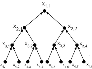
We first need some notation for T2(r). This will help to quickly recognize on which row each node is located. Let

Xij denote the i-th node on the j - t h row of the binary tree.

The Figure 4.2 shows such a labelling for T2(3).

Although the proof of the following lemma is folklore, we include it for completeness.

58 4. PAGERANK AND IN-DEGREE

A1,1

X

2,lf£ i l

y y y y 3,1 3,2 3,3 3,4

FIGURE 4.2. The binary tree T2(3) with xitj labelling.

L E M M A 4.2.1. Fix an integer r > 1.

(1) For 0 < i < r, the number of nodes on the i-th row

(assuming the root to be the 1st row) of the binary treeT2{r), is 2i~l.

(2) The binary tree T2{r) has order n — 2r — 1.

We note that all throughout this chapter we assume the binary tree to be a full binary tree, meaning that all of the leaves are on the same level and every non-leaf node has two children.

Proof: For item (1), we perform induction on i. For the

base step of the induction, consider the first row of nodes in

T2(r). As i = 1, hence, 2l _ 1 = 2° = 1. But there is exactly

4.3. CALCULATING THE STATIONARY DISTRIBUTION 59

The induction hypothesis assumes that on row i, we have 2'™1 nodes. Moving to the row i + 1, every node in row i

has two children (since the binary tree is full) and so the number of nodes on row i + 1 is twice the number of nodes on row i:

#(nodes on row i-\-\) = 2 x #(nodes on row i)

= 2 x 2i _ 1

= 2 \

For item (2), the total number of nodes in a full binary tree T ^ r ) , is counted by adding up the total number of nodes on each row. Hence:

\T2(r)\ = 21+ 22 + 23 + . . . + 2r r—1

=

E2"

=

2

- l . •

Calculating the exact PageRank vector for the binary tree would require us to compute all the powers of the dense

60 4. PAGERANK AND IN-DEGREE

Google matrix. As we are presently not able to perform this calculation, we decided instead to calculate the stationary distribution of a uniform random walk on the binary tree. As PageRank is the stationary distribution of the uniform random walk with teleportation, our results are suggestive of the actual PageRank values. The proofs in this chapter are original work.

A

AA:AA

F I G U R E 4.3. An arbitrary binary tree

A binary tree is depicted in Figure 4.3. The adjacency matrix (namely P i ) for the binary tree has the following

4.3. CALCULATING THE STATIONARY DISTRIBUTION structure. / 0 0 0 0 ^ 1 0 0 . . . 1 0 0 . . . 0 1 0 . . . 0 1 0 . . . 61 P i =

The matrix P i contains a nice pattern: starting from the second row, every two consecutive rows are equal. The next pair of rows results by a single shifting of the previous pair of rows to the right. For X ^ r ) , this pattern continues until the l's reach the (2r _ 1)-th column of the matrix. Since the

leaves of the tree have zero in-degree, the matrix will have a rectangular block of zeros of size (2r — 1) x 2r _ 1 on its

right side. The relative simplicity of this pattern allows a rigorous analysis of the uniform random walk on T2(n).

Consider the P2 matrix for T2(r). Recall that the P2

matrix is just P i without zero rows. In the binary tree, the root or the node x\^_ is the unique dangling node, where the random surfer would become stuck in the uniform random walk. Hence, we will assume that the root is pointing to

62 4. PAGERANK AND IN-DEGREE

all other nodes in the graph; this assumption turns P2 into

a stochastic matrix. The P2 matrix for the binary tree is therefore, ' 1/n 1/n .. . 1/n » 1 0 0 . . . 1 0 0 . . . 0 1 0 . . . 0 1 0 . . . M = P2 = V ; • ; where n = \V(T2(r))\. Throughout, let

M

6 — J n . l ~~

• • /

w

We now state the main results of this section

T H E O R E M 4.3.1. Let H be the P2 matrix of the binary tree X ^ r ) . Fix k a positive integer. Define [Hfc] • to be the sum of the column corresponding to the node xp^. For all

4.3. CALCULATING THE STATIONARY DISTRIBUTION 63

k > 1 and 1 < p < r,

where 1 < i < j < 2P~1. In particular, the column sums of any two nodes on the same row in T2{r) are equal.

T H E O R E M 4.3.2. Let H be the P2 matrix of the binary

tree T2(r). For all k > 1, 1 > i > j > 2v~l and 1 < p < r — 1, we have that

[H }Pjl = 2[H }p+ij + - [ H ]i;i;

ft/

where n = 2r — 1.

Note that -[H]i,i does not depend on either p or j . We defer the proofs of Theorem 4.3.1 and 4.3.2 until the fol-lowing section. We have however, the folfol-lowing corollary.

C O R O L L A R Y 4.3.3. Let s be the stationary distribution

vector of the P2 matrix of the binary tree T2(r).

(1) For any two nodes on the same row of T2(r), the

corresponding entries in s are equal.

(2) For all 1 < p < r — 1, the entry of s corresponding

64 4. PAGERANK AND IN-DEGREE

the entry corresponding to any of the nodes on the (p + l)-st row of s.

Proof: For the proof of (1), by definition we have that

(4.3) sT = lim erHt.

t—»oo

Now apply [•]-,• to both sides of (4.3), representing the sum of the j - t h column (or as in this case, the j-th element of the vector) on both sides of the limit:

[sr],- = [ l i m e ^ H ' b

t—>oo

= n m [ eTHt]i

t—*oo

= l-limlH*],-.

Note that [s]j = [e^H*]j represents the j-th. element of the vector. By Theorem 4.3.1, since H is the P2 matrix of the binary tree T2(r), for all t and for 1 < i, j < 2P~1,

[H]p,i = [H ]p,j.

But the column sum [H*]P)i represents the stationary value