Timing of Transients : Quantifying Reaching Times and Transient Behavior in Complex Systems

(1)

This content has been downloaded from IOPscience. Please scroll down to see the full text.

Download details:

IP Address: 139.133.148.27

This content was downloaded on 10/08/2017 at 08:41 Please note that terms and conditions apply.

Timing of transients: quantifying reaching times and transient behavior in complex systems

View the table of contents for this issue, or go to the journal homepage for more 2017 New J. Phys. 19 083005

(http://iopscience.iop.org/1367-2630/19/8/083005)

Timing of transients: quantifying reaching times and transient

behavior in complex systems

Tim Kittel1,2

, Jobst Heitzig1

, Kevin Webster1

and Jürgen Kurths1,2,3

1 _{Potsdam Institute for Climate Impact Research, Telegrafenberg A31}_—(_PO₎_{Box 60 12 03, D-14412 Potsdam, Germany} 2 _{Institut für Physik, Humboldt-Universität zu Berlin, Newtonstraße 15, D-12489 Berlin, Germany}

3 _{Institute for Complex Systems and Mathematical Biology, University of Aberdeen, Aberdeen AB24 3UE, United Kingdom}

E-mail:[email protected]

Keywords:early-warning signals, complex systems, nonlinear dynamics, ordinary differential equations, stability against shocks Supplementary material for this article is availableonline

Abstract

In dynamical systems, one may ask how long it takes for a trajectory to reach the attractor, i.e. how

long it spends in the transient phase. Although for a single trajectory the mathematically precise

answer may be inﬁnity, it still makes sense to compare different trajectories and quantify which of

them approaches the attractor earlier. In this article, we categorize several problems of quantifying

such transient times. To treat them, we propose two metrics, area under distance curve and regularized

reaching time, that capture two complementary aspects of transient dynamics. The

ﬁrst, area under

distance curve, is the distance of the trajectory to the attractor integrated over time. It measures which

trajectories are

‘reluctant’, i.e. stay distant from the attractor for long, or

‘eager’

to approach it right

away. Regularized reaching time, on the other hand, quantiﬁes the additional time

(

positive or

negative

)

that a trajectory starting at a chosen initial condition needs to approach the attractor as

compared to some reference trajectory. A positive or negative value means that it approaches the

attractor by this much

‘earlier’

or

‘later’

than the reference, respectively. We demonstrated their

substantial potential for application with multiple paradigmatic examples uncovering new features.

1. Introduction

In complex dynamical systems, the importance of a trajectory’s transient, i.e. the part of the trajectory distant from the attractor, has been identified in physics research as well as in various otherfields. Different phenomena during the process of magnetization for various materials, in particular the domain growth, have been studied extensively[1–3]. In laser physics, it was possible to derive analytical results matching the transient phases of different lasers[4,5]. In kinetic theory, there has been research on non-equilibrium approaches for more than a century by now[6]. Other modern areas of statistical physics have emphasized the importance of transient dynamics, too, e.g. in social systems[7]and transient phases between jam and free-flow phases in vehicular traffic[8].

Even outside of the directﬁeld of physics, but still within the scope of complex dynamical systems, a focus on transient dynamics has been developed recently. Hastings[9]made a call for more transient analysis of

ecological models. An example of this was given by vanGeest[10], describing macrophyte-dominated states of lakes as non-equilibrium states. In medicine and biology, epilepsy is seen as a transient phenomenon and much work has been done[11,12]. In economics, a transient analysis complementing the asymptotic analysis proved to be fruitful, particular supporting with the stability analysis and understanding how to reach the equilibria

[13]. Climate change is often seen as a transition to a new situation, i.e. a transient change to a new attractor

[14–16]. Closely related, discussions in sustainability sciences are on transient dynamics because they refer to transformations from and to sustainability. Important key topics are the Anthropocene[17–19], particular the great acceleration[20], and planetary boundaries[21,22].

OPEN ACCESS RECEIVED 16 November 2016 REVISED 20 June 2017 ACCEPTED FOR PUBLICATION 23 June 2017 PUBLISHED 7 August 2017

Original content from this work may be used under the terms of theCreative Commons Attribution 3.0 licence.

Any further distribution of this work must maintain attribution to the author(s)and the title of the work, journal citation and DOI.

(3)

An important emphasis onlong transientshas been made in[10,15,23]. With this term, they refer to trajectories where the relevant and observable phenomena/states, e.g. macrophyte-covered lakes or desert states of the Earth system, are away from the actual attractor, but in the transient phase where a trajectory may stay for a substantial amount of time.

Hastings[9]stressed the importance of different time scales and pointed out how the transient dynamics can be very different and much more interesting than the asymptotic behavior. In addition, he explained how saddles play a central role by inducing long transients. This has been demonstrated in a study by Anderiesetal

[15]in the context of sustainability science. The‘interacting planetary boundary’[21,22]has been deﬁned by whether states take‘long’to the attractor or not. This idea leads precisely to the main question for this article

‘How can we properly quantify the time to reach a system’s attractor?’, i.e. associate meaningful numbers with it. This study is meant as a methodological step in direction for applications in real-world systems. So in the following, we focus on being able to do numerical estimations while analytical results are only given to understand general properties.

Often, a trajectory is divided arbitrarily in a transient part and the asymptotics close to the attractor. So we split the main question into two sub-questions:(a)‘What are the problems of these current/intuitive methods to quantify transient time?’and(b)‘How can we mend them?’.

To answer thefirst question, we work out four essential problems one is confronted with:(I)infinite reaching time: the attractor is not reached infinite time for a large class of physically relevant systems;(II)physical interpretation: it is unclear how to define precisely‘when the transient is over’, so it is ambiguous where to divide between the transient and the asymptotics;(III)discontinuities: when having parameter dependence, small changes in the parameter often induce a large(noncontinuous)effect on the measured quantity; and(IV) non-invariance: the results depend on the choice of coordinates. Problem(IV)is particularly important, as a result should be a property of the dynamical system and thus independent of the choice of coordinates, i.e. invariant

(or correctly transforming)under smooth transformations of the state space(see‘smoothly equivalent’in[24]). Then, we approach question(b)by formulating two metrics,area under distance curve(D)andregularized reaching time(TRR). Theﬁrst one is the integral over the distance to the attractor along the trajectory, and has a

physical dimension of time times distance. It measures which trajectories arereluctant, i.e. stay distant from the attractor for long, oreager, i.e. approach it right away. The second one,TRR, is deﬁned by the difference between

the reaching times for the trajectory of interest and a reference trajectory. Thus, it takes a different point of view, actually measuring a time. The idea is that even though the actual reaching times are infinite(problem(I)), their difference is typicallyfinite. So, we can compare trajectories approaching the attractor and define the notions

earlierandlater.

We chose four examples to illustrate different features of these metrics. Weﬁrst use a linear system to understand how the metrics act generally and to observe the divergence ofTRRon the strong stable manifold

particularly. Also, due to the system’s simplicity, analytical solutions are possible. We then use a global carbon cycle model[15]and a model of a generator in the power grid[25]to apply the ideas to somefirst real world systems. Ourfinal example, the chaotic Rössler oscillator, demonstrates that one can apply these methods to more complex attractors also, in this case a chaotic one. The chosen examples are rather well-understood. So they are good testing cases for the metrics, while their complexity still needs numerical approaches for a proper quantification of reaching times.

Finally, a detailed discussion on how far the two metrics solve the aforementioned problems is given, followed by a summary and an outline of future research.

The remainder of this article is structured as follows. After stating the four essential problems of reaching time deﬁnitions in section2, we illustrate them with a small example. Then, we present the two metrics in section3and apply them to examples in section4. Next, we give a detailed discussion on how far the metrics solve the essential problems in section5. Finally, we close with a summary and an outlook. Additional

information that can be found the supplemental material is available online atstacks.iop.org/NJP/19/083005/ mmediareferenced within the article with the preﬁx‘Suppl. Mat.’.

Assumptions and notations.We assume a general, deterministic and autonomous dynamic system given by the differential equation

x˙=f x( ) xÎX ( )1

with ann-dimensional state spaceX₌_n_{and the right-hand side}₍_rhs₎_f₍_x₎_{. Usually, we use}_x_{to denote an}

arbitrary statexÎX, and refer to speciﬁc/ﬁxed states with letters as superscripts, e.g.xa_,_xb_{, and}_xref_{. The}

components of a state are written with subscripts, sox=(x0,x1,...,xn-1)andxa=(x0a,x1a,...,xna-1). The

words‘point’and‘state’are used synonymously for the elements ofX. We assume the system(1)to have at least one attractorÍXwith a basin of attraction ÍX. In case the system has more than one attractor, the

(4)

For convenience, we will make heavy use of the time-evolution operatorjwherej(t x, )is the state after starting at some pointxand letting the system evolve for some timet0. Hence

x x t t x f t x 0, and , , . 2 j = ¶j j ¶ = ( ) ( ) ( ( )) ( )

When we speak of‘quantifying the transient time’we mean toﬁnd a functionX⟶, a‘metric’, that gives a reasonable number for the time a trajectory spent in transient phase for each initial conditionxÎ.

Additionally, within the article we assume the asymptotics of the system to be understood as we want to focus on the transient only.

2. The problems of reaching time de

ﬁ

nitions

In this section, we introduce four essential problems. They need to be addressed when aiming to quantify the transient time to reach an attractorin a system of type(1). Then, we illustrate them with an example model.

(I) Inﬁnite reaching time.A basic property of a large class of complex systems is that trajectories reach the attractor in inﬁnite time only. That includes even steady states or limit cycles and most systems of ordinary differential equations with smooth rhs functions. This is the fundamental problem why the analysis made in this article is necessary.

(II) Physical interpretation.It is far from being obvious what the terms‘close to the attractor’or‘when the transient is over’means. Often, this is tackled by using some arbitrary thresholdòto deﬁne what is a‘small distance’to. But because of problem(I), the time to reach thisò-neighborhood typically diverges for0. So the result depends strongly on the value ofò. Note that the focus of this article is toquantifythe transient time to reach the attractor. So we want to associate meaningful numbers and need to treat this problem.

(III) Discontinuities.When deﬁning a metric to quantify the transient time to reachusing some

parameters e.g.ò, the result might depend discontinuously on the parameter. Usually, we want results to change smoothly and, if possible, weakly to changes of the parameter. If there is a discontinuous dependence, then we would expect there to be a corresponding speciﬁc property of the system that introduces this behavior.

(IV) Non-invariance.Our focus is on real-world systems. So the transient time should be a general property of the system, and not dependent on the chosen variables or coordinates to represent it. These coordinates correspond to a point of view on the system only. In other terms, invariance under change of coordinates should be given.

Example.While the aforementioned problems are of general nature, we illustrate them next using the example system

x 1 x bx x a x a b

2 , 2 , 2, 0.3. 3

0= - 1 - 0 1= - 02 = =

  ( ) ( )

It has a stable focusxs_{= -}₍ a, 2 1₍ ₊b a₎₎_{as its only attractor, and a saddle}_xu₌₍ _a_{, 2 1}₍ _-_{b a}₎₎_.

This has been chosen deliberately simple but is still sufﬁcient to demonstrate all four problems. This way, we do not have to cope with problems inherent to the example system, like high-dimensionality or chaos.

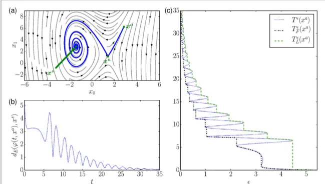
Itsflow is shown infigure1(a). For a chosen trajectory starting atxa₌₍2.8, 6.2₎₍_see_fi_gure₁₍_a₎₎_the

time-dependence of the Euclidean distance to the attractor

d t x, a ,x t x, a x 4

E( (j ) s)= j( ) · s ( )

is depicted infigure1(a). Two common metrics are the times when anò-neighborhood is entered thefirst and the last time. So we define the class of sets

T xa t d t x, a ,x , 5

E s



₍ ₎₌_{{ ∣} ₌ _{( (}_f ₎ _)} _{( )}

that invert the axes offigure1(b)as depicted infigure1(c) (blue dotted line).T x_{( )}a _{is the set of times when the} ò-neighborhood is entered or left. Furthermore, thefirst and last entry times are thenT xa infT xa

F( )= ( )and

T xa supT xa

L( )= ( )respectively. They are graphed inﬁgure1(c)also.

The inﬁnite reaching time(problem(I))is visible inﬁgure1(c)right away, asT xa ,T xa

F L

  _{ ¥}

( ) ( ) for

0

 . By deﬁnition, this implies that all elements inT x_{( )}a _{will approach}_¥_also.

Problem(II):T xa

F( )andT xL( )a depend heavily on the choice ofò. So a proper physical interpretation is

rather difﬁcult. The notions of‘close to the attractor’or‘when the transient is over’depend strongly onò. The strong discontinuities(problem(III))forT xa

F

_{( )}

andT xa

L

_{( )}

when changingòinﬁgure1(c)make the choice of a properòeven harder. The discontinuities arise because the trajectory will(for aﬁxedò)enter and exit the correspondingò-neighborhood several times. This behavior is caused by the complex eigenvalues of the system. It could be circumvented locally by choosing a different distance function, for instance

(5)

d x x P x x P a a , , 1 1 4 4 , 6 P s = -1 - s = _l _l + -  ⎜⎛ ⎟ ⎝ ⎞ ⎠ ( ) · ( ) ( ) where_l _{= -}b 2_ b2 4_-2 a

 are the complex eigenvalues of the linearization of(3)aroundxs.(This is

related to the · P-norm used in Suppl. Mat. Proposition 3.4.)Unfortunately, this is not so easy for more

complex attractors, e.g. the later treated chaotic Rössler system. However, we will present a pragmatic solution to this problem in section3.2.

Finally, using a different set of coordinates, i.e. smoothly transforming the system, gives different values for

T xa

F( )andT xL( )a , because the Euclidean distance is not invariant. Hence, the result depends on the set of

coordinates chosen for the system and is not invariant under coordinate transformations(problem(IV)). This dependence on the chosen distance is also known to appear inﬁnite-time dynamical systems and their stability[26].

3. Two complementary metrics

To treat the aforementioned problems, we devise two metrics for a general system as equation(1):area under distance curve(abbreviated asD)andregularized reaching time(TRR). They naturally lead to a transient analysis

from separate points of view as explained in the following.

3.1. Area under distance curve

Area under distance curve(D)comes from the idea that a trajectory stays distant from the attractor during the transient while it is close in the asymptotics. A distance functiond(· ·), is needed to have notions of‘far’and

‘close’and we deﬁneD D x dt d t x, , , 7 0 

ò

j = ¥ ( ) ( ( ) ) ( )

whereis the attractor with the basinandjthe time-evolution operator as in equation(2). So we look at the

cumulative distance to the attractor and remove the inﬂuence of the asymptotics. As(7)is the integral over the distance in time,Dis the area below the distance curve. A different point of view is that it is the time weighted by the distance.

Figure 1.The phase space for the example system equation₍3₎is depicted in₍a₎. Furthermore, the stable spiraling nodexs_{and the}

saddlexu_{are added. The trajectory}₍_blue₎_{starting at}_xa_{closely passes by}_xu_{before it}_ﬁ_{nally circulates in to}_xs_.₍_b₎_{shows the Euclidean}

distancedE(dotted, blue)of this trajectory to its attractorxsover timet. Theﬁrst longer dip betweent=1 andt=5 is the transient at

the(unstable)saddlexu_{while the oscillations afterwards are the spiraling around}_xs_.₍_c₎_turns₍_b₎_{around in order to show the}

dependence of the timeton some distanced=(dotted, blue)of the trajectory to the attractorxs_{. Secondly, there are multiple}

values ofòfor eachtso observables liket xa

F( )andt xL( )a need to be introduced.t xF( )a (dash–dotted, black)marks when theﬁrst time

theò-neighborhood aroundxs_{is entered and}_{t x}a

L( )(dashed, green)the last time. The implications, particularly the arising problems

(6)

AsDis deﬁned with the limit of an integral, a note on the convergence is due and can be found in the discussion in section5.

The distance functiondshould be between a point in state space and the attractor. Ifcontains more than just one element, it could be the inﬁmum of the distances to all points within. Choosing a tailor-made functiond(· ·), allows to adapt the metric to speciﬁc research questions, e.g. by lettingd x,( )represent some form of costs or damages due to being away from the attractor. For the idea ofDto work,dneeds to approach 0 around the attractor and be 0 on it.

Due to the integral representation,Dcan be estimated numerically directly from the trajectory assuming the attractor is known. The latter was taken as a prerequisite for this article as we want to emphasize the analysis of the transient.

Initial conditions with relatively high values ofDare called‘reluctant’and those with low values‘eager’. This terminology is used to emphasize that reluctant states go through large transients distant from the attractor, while eager states approach it directly.

By straightforward differentiation, we can compute the orbital derivative

tD j t x, d j t x, , , 8

¶

¶ ( ( ))= - ( ( ) ) ( )

meaning its value strictly decreases along theﬂow; a property we use later. Furthermore, this shows it to be a Lyapunov function[27]. Furthermore, using equation(8)and adding the conditionD x( )=0 " Îx is an alternative deﬁnition forD.

3.2. Regularized reaching time

The second idea,regularized reaching time(TRR), is based on time differences between trajectories. It can be

interpreted as the additional time(positive or negative)that a trajectory starting at a point of interest needs to approach the attractor after a reference trajectory has already approached it. A positive or negative value means that the trajectory at hand approaches the attractor by this much later or earlier, respectively, than the reference trajectory does.

To formalize this idea, we introducet x( )as the time a trajectory starting at an arbitrary statexneeds in order to reach anò-environment around the attractor. That means for some functionD:X ⟶0it holds

that

t x ,x , 9

_{= D}_{( ( ( )}_j  ₎₎ _{( )}

where we wantΔto be 0 on the attractor andD( (j t x, ))to be strictly and continuously decreasing int. This means, in equation(9),Δhas the role of a generalized distance function, measuring how far a point in state space is away from the attractor. Note thatj( ( )t x ,x)is the state after starting atxand evolving the system for a time

t x( ). Hence, equation(9)implicitly deﬁnest x( )to be the time at which anò-environment around the attractor, with respect to the generalized distance functionΔ, is entered.

Since the actual reaching times to the attractor are both inﬁnite,TRRis formally described as the limit for 0

 of the difference between how long the trajectory starting at some arbitrary statexand the trajectory starting at a chosen(ﬁxed)reference pointxref_{need to enter the corresponding}_ò_-environment

TRR x x; ref lim t x t x . 10 0 ref    = - ( ) ( ( ) ( )) ( )

For hyperbolicﬁxed points, we prove in Suppl. Mat. section 3 under mild conditions that there exists a class of choices forΔsuch that this limit exists for allxwithin the basin of attraction except the strong stable manifold and the attractor itself. We call the manifold associated to all Lyapunov exponents except the leading one the strong stable manifold. And, ifTRRexists, it is unique, i.e. independent of whichΔhas been chosen from the

class.

Furthermore, we show thatTRRis a parametrization of the strong stable foliation. Thus, after a smooth

change of coordinatesF, i.e. a diffeomorphism of the state space, the diffeomorphic image of the strong stable foliation will again parametrize the level sets ofTRRin the new variables. Therefore,TRRis invariant under such

transformations and it holds that

TRR( ( )F x ;F(xref))=TRR(x x; ref), (11)

where we obviously transformedxref_{, too.}

TRRrepresentsthe actual timeby how much a trajectory approaches the attractor later or earlier than the one

starting at the reference point, so we call states with relatively lowTRR‘early’and with highTRR‘late’.

Different choices ofxref₍_{that are not on the strong stable manifold or the attractor}₎_{result in additive}

(7)

TRR(x x; ref)-TRR(x x; ref¢ =) TRR(xref¢;xref). (12)

Because the rhs of equation(12)does not depend onx, different choices ofxref_{do not in}_ﬂ_{uence the structure of} TRRw.r.t.x. Thus central moments, i.e. ones invariant under shifts, are sensible for analyzingTRRover a

distribution of initial conditions in state space; especially the standard deviation proves useful for the examples below. In particular, for any choice ofxref_{it obviously holds that}_T _x _;_x ₀

RR( ref ref)= .

The reference point should not be chosen on the attractor because this givest x₍ ref₎₌0_{for any}_ò_{, but for} xÎX⧹the timet x( ) ¥for0. Vice versa, this means when having chosenxref _Î __then TRR(x x; ref)= -¥ " Îx . The same holds for the strong stable manifold.

In order to compute the orbital derivative T t y, ;x

t RR

ref j

¶

¶ ( ( ) ), we use equation(10)andﬁnd

tTRR t y, ;x lim tt t y, , 13 ref 0   j j ¶ ¶ = ¶ ¶  ( ( ) ) ( ( )) ( )

wherey ÎXis an arbitrary state and exchangeability of the limit and the derivative has been assumed. Next, we take the derivate with respect to timetin equation(9)forx=j(t y, ). Sorting the terms appropriately gives

t t t y t y tt t y 0= ¶ j  j , ,  j , 1 . 14 ¶ D + ¶ ¶ + ⎜ ⎟ ⎜ ⎟ ⎛ ⎝ ⎞ ⎠ ⎛ ⎝ ⎞ ⎠ ( ◦ ) ( ( ( )) ) · ( ( )) ( ) t x, j

D( ( ))is strictly decreasing intfor anyxÎX. So its derivative is t x, t x, 0

tD j = t D j < ¶ ¶ ¶ ¶

(

)

( ( )) ( ◦ ) ( )

and in particular non-zero. Hence, t t y, 1

t

 _j ₌

-¶

¶ ( ( )) , leadingﬁnally to the orbital derivative ofTRR

tTRR t y, ;x 1. 15

ref j

¶

¶ ( ( ) )= - ( )

This equation is actually rather natural, as the change of time to approach the attractor along the trajectory should exactly be the time passed. Also, this makes it a Lyapunov function[27].

To use equation(15)as an alternative deﬁnition we need another constraint. Because ofTRR(x x; ref)=

x 

-¥ " Î , this cannot be done on the attractor(in contrast toD). In case of hyperbolicﬁxed points, it follows directly from Suppl. Mat. Proposition 3.7 thatTRRis a parametrization of the strong stable foliationss,

whose deﬁnition is recalled in Suppl. Mat. Theorem 3.6. So we can use the constraint that

TRR(x x; ref)=0 " Îx refss , where we callssref =ss(xref)thereference leafcontainingxref. For more

complex attractors, a generalized condition needs to be found and this is part of the outlook.

Suppl. Mat. Proposition 3.4 provides the convergence ofTRRin equation(10)for hyperbolicﬁxed points

only. When thinking about more complex attractors that may arise in real-world examples the question of convergence comes up again. A general idea whyTRRshould converge with a well chosenΔin this case, too, is

that in the asymptotics, trajectories will‘behave similarly’because they are close to the attractor. So, for two very small1>2, the time difference to enter the2-environment after entering the one of1should be roughly the

same, independent from where a trajectory started. Hence, for two statesxandxref_{we can assume}

t2_{( )}x -t1_{( )}x »t2₍xref₎-t1₍xref₎_implying_t2_{( )}_x -_t2₍_xref₎»_t1_{( )}_x -_t1₍_xref₎_{. This suggests that the}

limit in equation(10)might exist. So a crucial problem is toﬁnd an appropriate function forΔin order to get an estimation forTRR.

Estimation ofTRR. Theﬁrst idea for aΔwould be the inﬁmum of the Euclidean distance to the points in the

attractor. Basically, this means thattshould be replaced byT_ForT_Lfrom section2. This would give a very coarse estimation but is probably not the correct choice as the condition ofΔbeing strictly decreasing along the

ﬂow is in general not fulﬁlled.

A pragmatic choice ofΔisD, the area under distance curve. It fulfills both conditions demanded forΔ(see section3.1)when using fordthe infimum of the Euclidean distance to the attractor points. Hence, we can define

t xD( )as the time until theD(equation(7))of the trajectory’s remainder isò-small

D t x_D ,x dt d t x, , . 16 tDx    

ò

j j = ( ( ( ) ))= ¥ ( ( ) ) ( ) ( )

Note that the ideas forDandTRRare generally independent and the usage ofDin this case is purely because it

fulﬁlls the above mentioned conditions. So it is a good, pragmatic choice.

UsingtD deﬁned in equation(16)as the time-functiontin equation(10)for the estimation ofTRR, our

numerical results show that this idea is sensible for more complex attractors, e.g. in the Rössler system below.

4. Examples

In order to demonstrate the applicability of the metrics, we selected four examples with differing properties and increasing complexity.

(8)

4.1. Linear system with two different time scales

Even though we want to focus on going in the direction of application to real-world systems, understanding some features in a basic linear system proves useful. For general systems,TRRandDcan be tackled numerically

only. But a linear system can be solved analytically and explicit expressions for both metrics were found. We will

ﬁrst analyze both metrics for a general linear system and then discuss a chosen example.

TRRfor a general linear system.For a hyperbolically stable linear system with a(complex-)diagonalizable

matrixA_În n´ _{and the}_ﬁ_{xed point}_xf_{at the origin,}

x˙=A x,· (17)

we decomposex _in i iv 01a

= å=- with coefﬁcientsa0,...,an-1in the eigenvector basisv0,...,vn-1with eigenvalues

,..., n

0 1

l l- _{sorted in descending order by real part. We assume in particular}_l0_{to have a strictly larger real part}

than_l1_{and multiplicity one. Hence we can apply Suppl. Mat. equation}₍₁₀₎_{derived in the Suppl. Mat. and get}

TRR x x; ref 1 ln , 18 0 0,ref 0 l a a = ( ) ( )

where_a0,ref_{is the}_a0_coef_ﬁ_{cient for the reference point}_xref_._a0,ref_{should be non-zero, i.e.}_xref_{should not be on}

the strong stable manifold.

Note that Suppl. Mat. Proposition 3.4 gives the uniqueness of this result independent of the choice ofΔ. In equation(18),TRRdepends only ona0, meaning the projection ofxon the eigenvector corresponding to

the least stable eigenvalue_l0_{. While this might be counter-intuitive in the beginning, it can be explained: the}

contributions from all other eigenvalues are vanishing because they decay faster than_l0_{by de}_ﬁ_{nition. So for a}

linear system, only the contribution from_l0_{remains. Also, on the strong stable manifold where}_a0₌₀_{, the}

values forTRRgo to-¥which we mentioned already in section3.2for general systems.

Dfor a general linear system.Taking the system(17)and choosingd x( ,{ })xf =d x xE( , f 2) the squared

Euclidean distance, we calculateDdirectly by using the deﬁnition equation(7)

D x v v. 19 i j n i j i j i j , 0 1 _* *

å

_la a_l = -+ = -( ) ( ) ( ) ( ) ( ) †

Therefore, in case ofD, all eigenvalues contribute, contrary toTRR. But they are weighted as can be seen in the

denominator. In case ofAbeing symmetric, this formula can be reduced toD x 1x A x 2

1 

=

-( ) .

TRRfor an example linear system.We choose then=two-dimensional linear system

x 1 0 x

4 2 20

= -

(

_-

)

˙ · ( )

with a stable and a strong stable eigenvalue and corresponding eigenvectors

v v 1, 1 4 and 2, 0 1 . 21 s s ss ss l = - =

( )

l = - =

( )

We choose the reference point to bexref ₌₍1, 1₎_{. Identifying}_l0₌_ls_,_v0₌_vs_implies 0 _x 0

a = . Then, using equation(18)gives

TRR(x x; ref)=ln(∣ ∣)x0 . (22)

This result is also visible in the numerical estimation inﬁgure3(c); the values ofTRRchange only in the direction

ofx0. The coloring describes the values of the metrics(see the colorbar in the right of theﬁgures)and the green

star representsxref_.

In order to get a better feeling for these metrics, we have chosen two exemplary initial conditions, an early-eagerone and alate-eagerone, and plotted their trajectories’distance to the attractor over time inﬁgure2. We see an intuition forTRR: it can be interpreted as the time-shift between the original trajectory and the reference

trajectory until the asymptotics match. So we plotted both trajectories shifted to each other using the analytical result forTRRin equation(22).

D for an example linear system.AnalyzingDfor the example linear system in equation(20)gives

D x 11x x x x 6 1 4 2 3 , 23 02 12 0 1 = + + ( ) ( )

where equation(19)has been used. The numerical result inﬁgure3(a)conﬁrms this.

Inﬁgure2, the blue-shaded area corresponds to theDvalue which is the same in both cases of our particular choice. This choice was made in order to see how trajectories can have differingTRRvalues even if theDvalues

match.

The exponential lower bound that comes up in the scatter plotﬁgure3(b)can be calculated analytically by combining equations(22)and(23)

(9)

Figure 2.Theﬁgure shows for two exemplary initial conditions(a)xb₌₍0.8, 2.35₎_and₍_b₎_xc₌₍_{1.4, 0.24}₎_{the distance of the}

attractor over time₍blue curve₎in the linear example system of section4.1. The initial conditions have been chosen such that theD

value, which corresponds to the blue-shaded area, is the same for both trajectories,D x_{( )}b ₌D x_{( )}c ₌3.8_{. But the trajectory starting}

atxb_{approaches the attractor}_earlier_{than the reference trajectory}₍_{green in}₍_a₎_and₍_b₎₎_{, which in turn is}_earlier_{than the one from}_xc_, meaningT xb;x 0.22 T x ;x 0 T x xc; 0.34

RR( ref)= - < RR( ref ref)= < RR( ref)= + . In order to show this, the example trajectories

(blue)have been shifted in each plot by the value ofTRRwith respect to the reference trajectory(green). This demonstrates an intuition

behindTRR: it describes by how much one has to shift one trajectory so it matches the asymptotics of the reference trajectory.

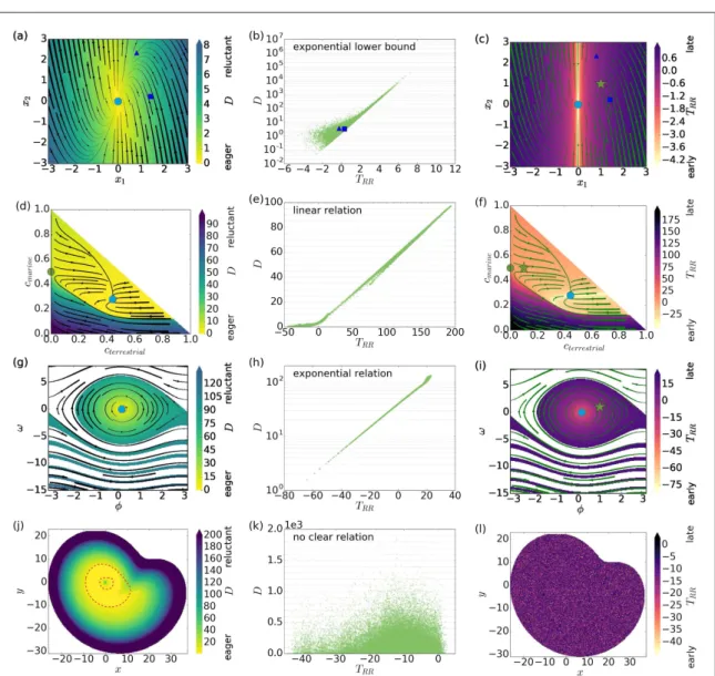
Figure 3.For the presented example systems(top to bottom: linear system, global carbon cycle, generator in a power grid, Rössler system)the two new metrics have been computed for each initial condition in the state space and marked with color, see left column

area under distance curve(D,D)and right columnregularized reaching time(TRR). The middle column shows their relations for the

particular system. The initial conditionsxb₍_triangle₎_and_xc₍_square₎_from_ﬁ_gure₂_{have been marked in}₍_a_)–(_c₎_{, too. As the Rössler} system is three-dimensional, the above plot depicts only a slice at_ﬁxedz_₌_0.6 where the boundary of the attractor_’s projection to this plane is shown in dashed red lines. As this is only a projection,Dis not 0 for all points within. For comparison, a graphical

(10)

D x 25 18e . 24 T x x 2RR ; ref  ( ) ( ) ( )

4.2. Global carbon cycle

The second example has been chosen to take a step in the direction of real-world examples. It is a conceptual model of the global carbon cycle proposed by Anderiesetal[15]. We use the pre-industrialization version. It consists of three dynamical variables, the terrestrial, marine and atmospheric carbon stocks, denoted by

ct=cterrestrial,cm=cmarineandca=catmosphericrespectively. Furthermore, the conservation of total carbon is

formulated in the constraintC=ct+cm+ca= const. Thus, we can reduce the system to 2 state variablesct

andcmand rescale the units such thatC=1:

c˙t=NEP(p r c, , t)-act, (25a)

c˙m=I c( a,cm), (25b)

where NEP is the net Eco-system production,pphotosynthesis,rrespiration,αharvesting parameter andI

diffusion; indirect dependencies have been omitted and more details are in[15,28]. As the full equations are rather lengthy, we put them in Suppl. Mat. section 1 and refer in the analysis to theﬂow that is drawn in

ﬁgures3(d)and(f)and theαparameter stated above. The whole phase space of equations(25a)and(25b)is the basin of the attraction of theﬁxed point in the middle marked by a blue dot; the dynamics is drawn as streams. The trajectories starting in the lower part have to pass by a‘desert-like’saddle(withct=0)at the left(green dot).

The color infigure3(f)depictsTRRand thefirstfinding is the splitting of the basin of attraction. The strong

stable manifold of the stable node becomes visible as a light beige line due to its low values ofTRR, i.e. as veryearly

states becauseTRR -¥. So it is the separatrix for the observed splitting. Also, the expected smooth increase

of the return times when distancing(along the trajectories)from the attractor can be observed.

Still, the splitting of the basin of attraction is visible for values ofcterrestrial<0.3, where it is only due to

quantitatively different behavior and the visible boundary is actually a rather sharp but still continuous transition.(The latter statement follows right from Suppl. Mat. Theorem 3.6 and Suppl. Mat. Proposition 3.7.) Looking atﬁgure3(f)one can also see that the boundary becomes more and more fuzzy for even smaller values of

cterrestrial, demonstrating that there is really a need for a quantitative analysis.

When applyingDto this model(ﬁgure3(d)), the splitting of the basin can be observed again. In contrast to

TRR, the strong stable manifold of the stable node is not visible becauseDcan be seen as a(by distance)weighted

time and the contributions from the asymptotic part where the difference in the Lyapunov spectrum matters are negligible.

Furthermore, we see a clear linear correlation of both metrics inﬁgure3(e)because all trajectories starting in the lower part have to pass by at the saddle on the left and spend a long time there.

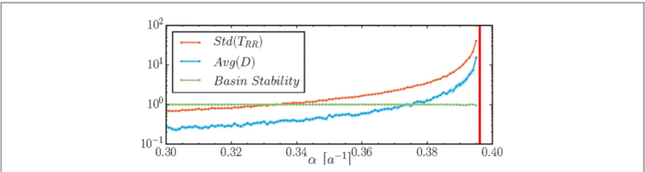
Both metrics work asearly-warning signals[14,29], too. When increasingα, corresponding to the harvest of terrestrial carbon, the system passes through a subcritical pitchfork bifurcation where the saddle becomes stable and the lower-left part of the phase space splits off. The divergences of the two metrics’statistics as seen in

figure4prove their prebifurcational sensitivity, while other systemic indicators like basin stability[30]do not change(up to numericalfluctuations, seefigure4). Note that in this example, a Lyapunov exponent analysis of the saddle would be able to predict the bifurcation due to the simplicity of the saddle also. However, in case of a more complex saddle, this would become arbitrarily difficult while this numerical estimation would still be possible for both metrics.

Figure 4.For theglobal carbon cyclein equations₍25a₎and₍25b₎, the mean ofDand standard deviation ofTRRare plotted(with their

5%–95% bootstrap error)and show a divergence before the parameterα(yearly human carbon offtake)reaches the bifurcation value (marked by the red line₎. For comparison Basin stability is shown, which doesnotshow any change because the size of the basin stays constant before the bifurcation.

(11)

4.3. Generator in a power grid

As the next example, we chose the swing equation in equation(26), a basic model describing the dynamics of a single generator connected to a large power grid[31]. It consists of two dynamical variables, the phaseθand angular frequencyω, both in a reference frame rotating at the grid’s rated frequency. The parameters of the system correspond to the net power productionP=1(at the node), the capacity of the transmission lineK=6 and dampeninga=0.1.

P K

, 2 2 sin . 26

f =w w_ = -aw- f ₍ ₎

In this form, which is used in electrical engineering[25,32], it is formally equivalent to a pendulum with constant driving and damping.

The stableﬁxed point at_ws₌0_, _arcsinP K

s

f = describes a state of synchronization. For the chosen set of parameters, the system exhibits another attractor: a limit cycle at larger positive values ofω. For negative values, the two basins of attraction are interleaved. A more detailed introduction and analysis can be found in

[25,31,33].

CalculatingTRRinside the basin of the stableﬁxed pointed(w qs, s)yieldsﬁgure3(i). There is basically no

color change away from the attractor, so we can see that a trajectory barely spends any time in the transient and goes quickly to the attractor. Analogously,ﬁgure3(g)forDleads to the same conclusion asTRR.

Comparing both metrics inﬁgure3(h)shows that they are closely linked. Note that this timeDis presented on a logarithmic scale, so the relation is exponential and what we see here is actually the inﬂuence of the linearized part of the system. The accumulation in the upper right corresponds to the initial conditions with lower values ofω. This means, they only go through a very short transient and spend most of their time in the part where the linearization holds.

The white parts in the phase spacesﬁgures3(g)and(i)correspond to the basin of attraction of the limit cycle. As this means the system is away from synchrony, the generators would usually switch off before reaching it. So we did not include it in the analysis.

4.4. Chaotic Rössler oscillator

Although we have proven the convergence ofTRRforﬁxed points only, we show with the chaotic Rössler system

[34,35]that both metrics are applicable to higher-dimensional and more complex attractors, too. The equations are

x = - -y z, y = +x ay, z= +b z x( -c), (27)

wherex,yandzare the coordinates in state space. While this naming convention is not in line with the rest of the article, it has been chosen as it is standard for these equations.

Figure3(l)shows a slice of the phase space with the standard parametersa=0.2,b=0.2,c=5.7 forTRR

and the expected sensitivity to initial conditions for chaos is observed:earlyandlatetrajectories lie closely together and the metricTRRhas low spatial correlation.

In contrast,Dshows infigure3(j)surprisingly smooth changes of an embryo-like shape. Because the focus of this article is on transient dynamics a new feature of the chaotic Rössler system is uncovered: while the attractor is chaotic, the basin of attraction is very regular.Dfocuses on the initial transient and the chaotic asymptotics isfiltered out. For comparison, the boundaries of the attractor’s projection have been added with dashed red lines infigure3(j)and depictions of the attractor are in Suppl. Mat. section2.

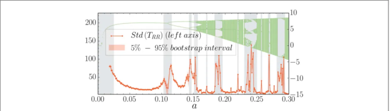
Furthermore,TRRcan be applied as an early-warning signal in this case, too. In order to demonstrate this, we

chose to varyaas it has a crucial influence on the system’s dynamics(see the bifurcation diagram infigure5 (green)). For values ofa<0.006(see[36])there is only a single stablefixed point. Ata»0.006a limit cycle emerges due to a Hopf bifurcation[36]. Fora>0.11, several period doublings are observed,finally leading to chaos fora>0.155. Even in the chaotic regime, further bifurcations can be observed.

Inﬁgure5, the standard deviation of theTRRdistribution from randomly chosen initial conditions inside the

basin of attraction is given. Due to the sensitive dependence on initial conditions, the reference value varies a lot and hence introduce shifts in the distribution that do not describe actual changes in the system’s dynamics. To remove this effect, it is crucial to use central moments like the standard deviation.

TRRis strongly sensitive to any qualitative changes in the dynamics of the system, incl. even chaos–chaos

transitions. Closely observingﬁgure5uncovers that there is a base-line with littleﬂuctuations atStd(TRR)»10

complemented with strong peaks. In the chaotic regime, the peaks correspond directly to qualitative changes. Also, we observe sensible changes during the period-doubling phase and a strong increase before the Hopf bifurcation ata»0.006, proving the usefulness as anearly-warning signal.

The abrupt downward peak ata»0.11is unexpected and more details are needed to clarify it. The other peaks correspond well with the transitions visible in the bifurcation diagram.

(12)

5. Discussion

In order to see how far the two proposed metrics answer the question‘How can we properly quantify the time to reach a system’s attractor?’we will go along the four essential problems that have been worked out in section2

for this discussion:(I)inﬁnite reaching time,(II)physical interpretation(III)discontinuities and(IV) non-invariance.

Area under distance curve (D)has been deﬁned as the cumulative distance to the attractor over time in order to emphasize the idea that a trajectory stays‘far’from the attractor in the transient while being close in the asymptotics. The distancedis not necessarily meant in the mathematical sense[37], but it only needs to approach 0 around the attractor and be 0 on it. In that way, it is possible to choose the appropriatedfor different research questions, e.g. asking about costs or damages. Even in these interpretationsDis a metric capturing the transient time, because there are only contributions when the trajectory is distant from the attractor, i.e. still in its transient phase. Another point of view is to seeDas the time to reach the attractor weighted by the distance.

We understand Problem(I), inﬁnite reaching time, as solved. For hyperbolic attractors anddbeing a mathematical distance function, the integral in equation(7)does converge. Trajectories approach the attractor exponentially in the asymptotics and the integral over the exponential envelope isﬁnite.

While this covers most systems relevant for real-world applications, in some very specific cases,Dmight be infinite. The asymptotic tail of the integral might not converge, i.e. the trajectory does not approach it‘fast enough’. This means, either this is the wanted result ordhas not been chosen appropriately. In thefirst case, it could be for example thatDwas computed for an initial condition that is not economically feasible, so the cost diverges. Furthermore, this would imply that even though the attractor is systemically stable, it is not

economically feasible to cope with small perturbations.

From a technical perspective a divergence inDcan be understood as indicating thatdhas not been chosen matching to the system. E.g. using the Euclidean distance andx 1x

2 3 =

-˙ where the solutions are

t x, sign x t x 1 2 j = + -( ) ( )

∣ ∣ ,Ddoes not converge. Another example is to take a linear systemx˙= -xwith

x<1. Usingd x, 0 x 1 ln = -( { }) ∣ ∣withd(0, 0{ })=0givesD ¥.

This can usually be solved by choosing an appropriated. E.g. choosing forx 1x 2

3 =

-˙ using

d x₍ , 0_{{ })} ₌exp_{( ∣ ∣ )}_-x-1 _and_d₍_{0, 0}_{{ })} ₌₀_gives_ﬁ_{nite values for}_D_.

Problem(II)is solved because there is no direct parameter. Still, as there is the indirect dependence onda discussion is necessary and given in comparison to theﬁrst and last entry time to anò-environmentT x_F( )and

T x_L( )respectively. For them, a small change inòwill have a huge impact on the measured times because for

0

 both values go to inﬁnity. Furthermore, if one would locally change the way how the distance to the attractor is measured, the values forT xF( )andT xL( )would change drastically, too.

BecauseDis deﬁned as the cumulativedover time, a local change indwill have only minor effects on the exact value, so even estimated functions fordwith some uncertainty can be used.

Problem(III), discontinuities, have been avoided inDby using the integral representation. Hence the function is even differentiable along theﬂow(see equation(8)).

We see Problem(IV), non-invariance, as solved, ifdhas been chosen with some meaning, e.g. economic damages. Then one can simply represent the economic damage function in the changed coordinates, because the meaning is independent of the coordinates. This reasoning is not mathematical but context-dependent. From a purely mathematical point of view, ifdis just any distance function, generally the result is not invariant under

Figure 5.The bifurcation diagram(green)of the Rössler system for varying the parameterain equation(27)was computed from the local maxima inzof the attractor andTRR(orange)shows a strong sensitivity to these qualitative changes. The gray background is used

(13)

change of coordinates as it depends on geometric features of the system. But as we want to go in the direction of real-world systems, a model-speciﬁc choice ofdis compulsory anyway.

Regularized reaching time(TRR)has been deﬁned as the difference in time to approach the attractor.

Problem(I), infinite reaching time, does not appear for all states in the basin of attraction except the attractor and the strong stable manifold. In case of the attractor, the trajectory will stay on it while trajectories from other points approach the attractor only; and, by definition, points on the strong stable manifold approach the attractor a lot faster, also in the asymptotics. So these infinities are actually reasonable results. Also, both are usually of a smaller dimension than the state space. Hence coincidently being there is unlikely, and these cases are rather irrelevant for real-world applications.

Problems(II)and(III)are intrinsically solved by avoiding parameters. The necessary choice ofxref

introduces a constant shift only while not changing the structure of the function. When looking at central moments ofTRR, i.e. ones invariant under shifts, this dependence on the choice ofxrefdisappears completely as

they would only shift the mean. So an analysis by changing the system’s parameters is possible. This has been done in the examples for the global carbon cycle and Rössler system andTRRhas been conﬁrmed as an

early-warning signal. This analysis can be seen as a systemic approach to the concept ofcritical slowing down(CSD)

[14,29,38]after a shock, i.e. an instantaneous and non-inﬁnitesimal perturbation, uncovering prebifurcational changes in the transient behavior. In contrast, CSD is usually done with(local)noise only. The usage of shocks has been developed in the context of Basin stability[30,31]and its extensions[23,39–42].

Problem(IV), non-invariance, is proven to be solved for hyperbolicﬁxed points. In case of more complex attractors, we can currently only deﬁne an estimation ofTRRwhich depends on geometric properties. So

invariance might not be given and more research due in that direction. An important step in that direction has been done by writing down the properties ofΔwhich imply that the necessary way of measuring how a trajectory approaches might not be local(exceptﬁxed-points). The used pragmatic choice ofD =D

demonstrates this as it basically says that the remainder of the trajectory should have anòsmall value ofDonly. An assumption that has been made during the proof of invariance ofTRRfor hyperbolicﬁxed points is: the

eigenvalue of the RHS’s Jacobian with the largest real-part is either unique and with multiplicity 1 or there are two that are complex conjugated to each other. However, this condition is not really constraining because we assume most real world systems fulﬁll it.

Comparison.The metrics have been applied to several examples and we will discuss a comparison between both metrics here. They are depicted inﬁgures3(b),(e),(h)and(k)and show different relations, as stated in the

ﬁgures. The exponential lower bound and the exponential relation for the linear system and swing equation respectively come mostly from the asymptotic behavior, in particular as the linear system does(by deﬁnition) not have any nonlinearities. Still the relations are different as the asymptotic behavior differs slightly, too, one being a node the other a focus. This shows that even though we clearly focus on the transient, it is actually important to be aware of the asymptotic behavior, too. And one cannot analyze the former without knowing about the latter.

In contrast, the linear relation for the global carbon cycle really points to the transient behavior only. It is due to the states passing by the‘desert-like’saddle. Finally, there seems to be no clear relation between both metrics for the Rössler example, pointing to the chaotic behavior. Still, both metrics have separately been useful,D

demonstrating the smoothness of the basin of attraction and the standard deviation ofTRRbeing sensitive to

qualitative changes of the system.

Other methods.When developing this research on measuring times to approach the attractor, we had the impression that there are two more common ideas, additionally to theﬁrst and last entry time. We do not intend to have a complete overview of all methods but would like to discuss these two shortly here. This part refers to a general system in the sense of(1).

Theﬁrst idea is to develop metrics based on characteristic times. These are usually deﬁned as the time until a quantity is reduced to1 eof its original value[43]. This quantity could be a distance to the attractor or a

coordinate. From this deﬁnition it already follows that they are subject to problem(IV). Also, even if the quantity is at1 eof its initial value, the trajectory might still be far away from the attractor and in its transient dynamics. Lastly, taking a one-dimensional linear system and assuming the quantity is the coordinate, the characteristic time is constant for all initial conditions. This is counter-intuitive when thinking about a time to approach the attractor.

The second idea for general systems is to use Lyapunov exponents[44]. They have units of inverse time and are invariant under changes of coordinates. However, they are actually a property of the attractor. So they do not capture the transient but only the asymptotics closely around and at the attractor.

(14)

6. Summary and outlook

In this article, we have treated the question:‘How can we properly quantify the time to reach a system’s attractor?’

First, we have worked out the four essential problems of quantifying the timing of transients in order to develop two new metrics,area under distance curveDandregularized reaching timeTRR. As the focus of this work

is meant to be on making aﬁrst step to real-world systems, we have applied the metrics numerically to four chosen examples systems, observing different features. Finally, we have discussed in detail how far the metrics treat the four essential problems.

With this approach, interesting features of the examples have been uncovered. Using the global carbon cycle, we have demonstrated the importance of the transient analysis, as the desert state is only a saddle but

nevertheless passing by there would lead to an extinction of humanity. The splitting of the basin of attraction is partially due to the strong stable manifold of the attractor but it continues for lower values ofcterrestrialwhere it is

only due to quantitatively different behavior demonstrating the need for quantitative methods. Particularly interesting is how the(central)statistics of our metrics are a systemic approach to the concept of CSD leading to an interpretation as early-warning signals, which we have demonstrated also. The independence of the choice of reference points has been achieved by the usage of central moments. In case of the generator in a power grid, most of the relevant dynamics seems to be dominated by the linearization of the equations around the focus. In order to prove the applicability to more complex dynamics, we have used our metrics on the Rössler system, too, and found the smoothness of the attractor’s basin withD. As the attractor itself is chaotic, this smoothness is surprising.TRRreacts strongly to the sensitivity to initial conditions of the chaotic system and one

might want to ask whether there is a relation to winding numbers when approaching the attractor. Still, its worth is displayed when varying theaparameter. This parameter has strong inﬂuence on the Rössler system’s

dynamics andTRRreacts strongly to the different bifurcations and even the chaos–chaos transitions, proving

again its worth asearly-warning-signal.

We have not performed any comparative analysis with the mentionedﬁrst- and last-entry-time approaches because these behave inconsistently and their quantitative results are arbitrary, as discussed at length in section2.

The detailed discussion on the two metrics have showed that, while they do treat the four essential problems, they do not fully solve them and further investigation is needed. Also, they come from two very different basic ideas so the comparison showed that they really measure independent features but can improve the

understanding of a system by combining them. For both metrics, we have showed that they are Lyapunov-functions. While some properties have already been used in the article, these deﬁnitions in terms of orbital derivatives may be a rich groundwork for the next steps.

Four directions of immediate future research are due:

(1)Working on the deﬁnition ofTRRusing the Lyapunov function properties. This step is crucial in order to

further the understanding of transient analysis and needs to take the attractor into account as well. Hence, the analysis of more complex attractors and basin shapes, e.g. riddled basins, is part of this.

(2)Applying the current deﬁnition of the metrics, in particular using the estimation ofTRRwithD =D, to

understand the implications and the precise use cases better. Furthermore, their relations to topological structures, e.g. in complex networks[45], need to be worked out in detail. This part, even though complementary, should be done in accordance with the results in(1).

(3)On the numerical side, it is important to introduce more sophisticated methods of Lyapunov function estimations, where a starting point is the work by Giesl and Hafstein[46]. The curse of dimensionality is going to be a problem for network systems, hence methods for estimation of these metrics’statistics in such kinds of systems induce a need for developing speciﬁc algorithms.

(4)Comparison of the timing of transients in model output and observation data as the new observable time is now available.

Acknowledgments

The authors thank the anonymous referees for their detailed and constructive feedback.

This paper was developed within the scope of the IRTG 1740/TRP 2011/50151-0, funded by the DFG/ FAPESP. This work was conducted in the framework of PIKsﬂagship project on coevolutionary pathways

(COPAN). The authors thank CoNDyNet(FKZ 03SF0472A)for their cooperation. The authors gratefully acknowledge the European Regional Development Fund(ERDF), the German Federal Ministry of Education and Research and the Land Brandenburg for supporting this project by providing resources on the high performance computer system at the Potsdam Institute for Climate Impact Research. The authors thank the developers of the used software: Python[47], Numerical Python[48]and Scientiﬁc Python[49].

(15)

The authors thank Sabine Auer, Karsten Bölts, Catrin Ciemer, Jonathan Donges, Reik Donner, Jasper Franke, Frank Hellmann, Jakob Kolb, Chiranjit Mitra, Finn Müller-Hansen, Jan Nitzbon, Anton Plietzsch Stefan Ruschel, Tiago Pereira da Silva, Francisco A Rodrigues, Paul Schultz, and Lyubov Tupikina for helpful discussions and comments.

References

[1]Barkema G, Marko J and De Boer J 1994Europhys. Lett.26653 [2]Gaulin B D and Spooner S 1987Phys. Rev. Lett.58668–71 [3]Chou Y C and Goldburg W I 1979Phys. Rev.A202105 [4]Fiutak J and Mizerski J 1980Z. Phys.B39347–52

[5]Tang C, Telle J and Ghizoni C 1975Appl. Phys. Lett.26534–7

[6]Krapivsky P L, Redner S and Ben-Naim E 2010A Kinetic View of Statistical Physics(Cambridge: Cambridge University Press)

[7]Castellano C, Fortunato S and Loreto V 2009Rev. Mod. Phys.81591 [8]Chowdhury D, Santen L and Schadschneider A 2000Phys. Rep.329199–329 [9]Hastings A 2004Trends. Ecol. Evol.1939–45

[10_]Van Geest G, Coops H, Scheffer M and van Nes E 2007Ecosystems1037_–47 [11_]Schaffer W M, Kendall B, Tidd C W and Olsen L F 1993Math. Med. Biol.10227_–47

[12]Fisher R S, Boas W v E, Blume W, Elger C, Genton P, Lee P and Engel J 2005Epilepsia46470–2

[13]Fisher F M 1989Disequilibrium Foundations of Equilibrium Economics(Cambridge: Cambridge University Press)

[14]Lenton T M 2011Nat. Clim. Change1201–9

[15]Anderies J M, Carpenter S R, Steffen W and Rockström J 2013Environ. Res. Lett.8044048 [16]Heitzig J, Kittel T, Donges J F and Molkenthin N 2016Earth Syst. Dyn.721–50

[17]Crutzen P J 2002Nature41523 [18]Steffen Wet al2011Ambio40739–61 [19]Waters C Net al2016Science351aad2622

[20]Steffen W, Broadgate W, Deutsch L, Gaffney O and Ludwig C 2015Anthropocene Rev.281–98 [21]Rockström Jet al2009Ecol. Soc.1432

[22]Steffen Wet al2015Science3471259855–1–10

[23]van Kan A, Jegminat J, Donges J F and Kurths J 2016Phys. Rev.E93042205–1–7 [24]Kuznetsov Y A 2013Elements of Applied Bifurcation Theoryvol 112(New York: Springer)

[25]Weckesser T, Jóhannsson H and Østergaard J 2013 Impact of model detail of synchronous machines on real-time transient stability assessmentBulk Power System Dynamics and Control-IX Optimization, Security and Control of the Emerging Power Grid, (IREP) Symp.

(IEEE)pp 1–9

[26_]Bhat S P and Bernstein D S 2000SIAM J. Control Optim.38751_–66

[27]Giesl P 2007Construction of Global Lyapunov Functions using Radial Basis Functions(Berlin: Springer)

[28]Heck V, Donges J F and Lucht W 2016Earth Syst. Dyn.7783–96

[29]Scheffer M, Bascompte J, Brock W A, Brovkin V, Carpenter S R, Dakos V, Held H, Van Nes E H, Rietkerk M and Sugihara G 2009

Nature46153–9

[30]Menck P J, Heitzig J, Marwan N and Kurths J 2013Nat. Phys.989–92 [31]Menck P J, Heitzig J, Kurths J and Joachim S H 2014Nat. Commun.51–8 [32]Yuan Y, Kubokawa J and Sasaki H 2003IEEE Trans. Power Syst.181094–102 [33]Schultz P, Heitzig J and Kurths J 2014New J. Phys.16125001

[34]Rössler O E 1976Phys. Lett.A57397–8 [35]Zgliczynski P 1997Nonlinearity10243

[36]Barrio R, Blesa F, Dena A and Serrano S 2011Comput. Math. Appl.624140–50

[37]Heitzig J 2002 Mappings between distance sets or spacesPhD ThesisUniversität Hannover

[38]Scheffer Met al2012Science338344–8

[39]Klinshov V V, Nekorkin V I and Kurths J 2015New J. Phys.18013004 [40]Hellmann F, Schultz P, Grabow C, Heitzig J and Kurths J 2016Sci. Rep.61–12 [41]Mitra C, Kurths J and Donner R V 2015Sci. Rep.51–10

[42_]Mitra C, Choudhary A, Sinha S, Kurths J and Donner R V 2017Phys. Rev.E95032317

[43_]Clark M M 2011Transport Modeling for Environmental Engineers and Scientists₍New York: Wiley₎

[44]CvitanovićP, Artuso R, Mainieri R, Tanner G and Vattay G 2016Chaos: Classical and Quantum(Copenhagen: Niels Bohr Inst.)

[45]Havlin Set al2012Eur. Phys. J. Spec. Top.214273–93

[46]Giesl P and Hafstein S 2015Discrete Continuous Dyn. Syst.B202291–331

[47]Van Rossum G and Drake F L Jr 1995 Python Reference Manual(Centrum voor Wiskunde en Informatica Amsterdam)

[48]Ascher Det al2001Numerical Python