RELOCATION OF THE RICH: MIGRATION IN RESPONSE TO TOP TAX RATE
CHANGES FROM SPANISH REFORMS
David R. Agrawal, Dirk Foremny
IEB Working Paper
2018/06
IEB Working Paper 2018/06
RELOCATION OF THE RICH: MIGRATION IN RESPONSE TO TOP TAX RATE CHANGES FROM SPANISH REFORMS
David R. Agrawal, Dirk Foremny
The Barcelona Institute of Economics (IEB) is a research centre at the University of Barcelona (UB) which specializes in the field of applied economics. The IEB is a foundation funded by the following institutions: Applus, Abertis, Ajuntament de Barcelona, Diputació de Barcelona, Gas Natural, La Caixa and Universitat de Barcelona.
The IEB research program in Fiscal Federalism aims at promoting research in the public finance issues that arise in decentralized countries. Special emphasis is put on applied research and on work that tries to shed light on policy-design issues. Research that is particularly policy-relevant from a Spanish perspective is given special consideration. Disseminating research findings to a broader audience is also an aim of the program. The program enjoys the support from the IEB-Foundation and the IEB-UB Chair in Fiscal Federalism funded by Fundación ICO, Instituto de Estudios Fiscales and Institut d’Estudis Autonòmics.
Postal Address:
Institut d’Economia de Barcelona Facultat d’Economia i Empresa Universitat de Barcelona C/ John M. Keynes, 1-11 (08034) Barcelona, Spain Tel.: + 34 93 403 46 46 [email protected] http://www.ieb.ub.edu
The IEB working papers represent ongoing research that is circulated to encourage discussion and has not undergone a peer review process. Any opinions expressed here are those of the author(s) and not those of IEB.
IEB Working Paper 2018/06
RELOCATION OF THE RICH: MIGRATION IN RESPONSE TO TOP TAX RATE CHANGES FROM SPANISH REFORMS *
David R. Agrawal, Dirk Foremny
ABSTRACT: A recent Spanish tax reform granted regions the authority to set income tax rates, resulting in substantial tax differentials. We use individual-level information from Social Security records over a period of one decade. Conditional on moving, taxes have a significant effect on location choice. A one percent increase in the net of tax rate for a region relative to others increases the probability of moving to that region by 1.7 percentage points. Focusing on the stock of top-taxpayers, we estimate an elasticity of the number of top taxpayers with respect to net-of-tax rates of 0.85. Using this elasticity, a theoretical model implies that the mechanical increase in tax revenue due to higher tax rates is larger than the loss in tax revenue from the out-flow of migration.
JEL Codes: H24, H31, H73, J61, R23
Keywords: Migration, Taxes, Mobility, Rich, Fiscal Decentralization David R. Agrawal
Department of Economics and Martin School of Public Policy & Administration, University of Kentucky & CESifo
E-mail: [email protected]
Dirk Foremny
Universitat de Barcelona &
Institut d’Economia de Barcelona (IEB) E-mail: [email protected]
* This project began while David Agrawal was a guest researcher at Universitat de Barcelona. He thanks
Universitat de Barcelona, along with the people associated with it, for their support. We thank the editor, Rohini Pande, and three referees for improving the paper. The paper benefited from comments by José Maria Durán, Dennis Epple, Alejandro Esteller-Moré, Gabrielle Fack, Aart Gerritsen, Steven Haider, James Hines, William Hoyt, Jordi Jofre-Montseny, Camille Landais, Andrea Lassmann, Thomas Piketty, Kurt Schmidheiny, Nathan Seegert, Danny Shoag, Joel Slemrod, Albert Solé-Ollé, Michel Strawczynski, Juan Carlos Suárez Serrato, Johannes Voget, Daniel Waldenström, David Wildasin, and Daniel Wilson as well as seminar participants at Case Western Reserve University, CESifo Venice Summer Institute, Centre for European Economic Research (ZEW), CESifo Conference on Public Sector Economics, ETH Zurich, International Institute of Public Finance, Michigan State University, National Tax Association, the Paris School of Economics, the Pontifícia Universidade Católica de Rio de Janeiro, Purdue University, the Universitat de Barcelona, the University of Kentucky, the University of Louisville, the University of Michigan, the MaTax Conference in Mannheim, Germany the PET 2016 Conference in Rio de Janeiro, and Universität Siegen. Dirk Foremny acknowledges financial support from the Fundación Ramón Areces and projects ECO2012-37131 and ECO2013-41310 (Ministerio de Economía y
High-income taxpayers may be literally “worth their weight in gold” to the government where they reside.1 As a means of tax avoidance, individuals may move in response
to tax differentials resulting from residence based local income taxes. Tax avoidance typically arises when taxable income can be shifted in a way that it becomes subject to a favorable tax treatment (Piketty and Saez 2013), and mobile taxpayers might simply relocate their tax residence to reduce their income tax burden. As a result of tax induced mobility by high-income taxpayers, governments may be unable to engage in progressive redistribution (Epple and Romer 1991; Feldstein and Wrobel 1998) and tax competition may intensify (Wildasin 2006). Despite the policy importance of analyzing taxation in an open economy setting, most studies have analyzed responses of taxable income (Feldstein 1999) although a recent literature on tax-induced mobility has emerged.
We provide evidence on migration resulting from a major Spanish tax reform and fiscal decentralization. In the early 2000s, all Autonomous Communities (regions or states) in Spain had the same top marginal tax rate. In 2011, Spanish regions began changing their top marginal tax rates in response to a federal reform that gave regions the authority to adjust rates and the corresponding tax brackets. In 2014, top marginal tax rates diverged across regions by as much as 4.5 percentage points. For an individual earning 300,000 Euros, this amounts to a tax differential of 10,000 Euros. These dispari-ties in regional top tax rates led the popular press to dub low-tax regions such as Madrid as “tax havens” or one of several “paradises on Earth.”
Research on migration requires linked data of individuals in the country of origin and destination, which is fairly complicated to obtain.2 Exploiting sub-national variation
is therefore an appealing alternative. However, personal income in most countries is taxed at the federal level and only a few countries tax personal income at the regional or
1The quoted phrase comes from Wildasin (2009), who writes: “at current prices ($900/oz.), an
average adult male’s weight-equivalent (190 lbs.) of gold is worth around $2.7 million. Under conservative assumptions about life expectancy and discount rate, the present value of taxes paid by very high income taxpayers can easily exceed this amount.”
2Klevenet al. (2013) and Akcigitet al. (2016) are notable exceptions. They focus on selected
sub-groups of the population for which the authors have been able to assemble the information needed without access to individual income data linked across countries. Bakija and Slemrod (2004), Moretti and Wilson (2017) and Young et al. (2016) are also noteworthy state level examples, but as discussed below state level income taxation is not always residence based in the United States.
local level (i.e., United States, Canadian provinces were granted the authority to set their own bracket and rates in 2001 (Milligan and Smart 2016), Swedish municipalities, Italian regions and municipalities, Swiss cantons and localities). Given the expected mobility and avoidance responses, some of these countries only allow for small differentials across jurisdictions by limiting the tax-setting power of state and local governments. In countries with more substantial autonomy, regional personal income taxes have been implemented decades ago and large administrative data are not available for time periods before their implementation. Further, in the U.S., income taxes are often employment-based rather than residence-based, which means that for local moves, individuals may change jobs rather than residence to reduce taxes (Agrawal and Hoyt 2018).3 The reform in Spain
granted substantial autonomy to the regions on a purely residence-based tax system. Tax administration remains with the national authorities which facilitates access to individual micro-data that is available before and after the decentralization.
We use individual Social Security data for a sample of the population of Spain (excluding Navarre and Basque Country, which are not included in the data) from 2005 to 2014 to study the migration decisions of the rich in response to this unique fiscal de-centralization. Our paper makes several contributions. First, we focus on all high income individuals rather than a select group of highly mobile individuals such as star scientists (Moretti and Wilson 2017; Akcigitet al.2016), athletes (Klevenet al.2013), or foreigners subject to preferential taxation (Kleven et al. 2014; Schmidheiny and Slotwinski 2015). In terms of the scope of the sample, Younget al. (2016) are the closest to our paper and utilize population level U.S. tax return data for all millionaires in the United State over a thirteen year period. Exploiting state-to-state migration of millionaires and an empirical design comparing millionaire populations at state borders, Younget al.(2016) concludes that although taxes matter, it is with only very small economic significance.4 Second, 3In the United States, 5.3 million individual have an interstate commute. Approximately 75 million
people live in metropolitan areas that cross state borders. Of these, approximately two-thirds live in MSAs that have an employment-based component to state and local income taxes.
4We make several contributions relative to Younget al. (2016). First, we study migration patterns
of the rich (above 90,000 Euros) and not just the very rich (millionaires). We also study migration in a setting where regional taxes are purely residence-based; in the United States, taxes may have a residence and employment-based component. Finally, we show heterogeneous effects by industry and occupation.
we study migration using a random sample of population level administrative data for a complete panel of all regions in a country; Young et al. (2016) have similar data and a single state analysis includes Young and Varner (2011).5 This administrative data
pro-vides us detailed information on industry and occupation that allows us to determine the generalizability of the prior literature focusing on specific occupations. We find signifi-cant effects of taxes on location choices, but an elasticity of the number of top taxpayers that is less than unity. We then contribute to the literature by using a theoretical model of revenues to simulate the implications of these elasticities for the fiscal authorities.
Discussion of taxing top incomes comes within the context of widening income inequality in many countries (Roine and Waldenstr¨om 2011). One discussed policy re-sponse to widening inequality is changing top tax rates. Bonhomme and Hospido (2017) document that earnings inequality in Spain declined from about 1995 to 2007, but that it has risen dramatically since 2007 and is back to its 1995 level. Studying mobility in Spain is especially important given the implications for redistributive tax policy. The mobility response – especially of high income taxpayers – is critical to understanding whether increasing progressivity at the regional level is a viable policy response to in-creasing inequality. Mobility in response to more progressive tax policy could threaten the ability to engage in redistribution given that the optimal degree of redistribution will decline as the mobility elasticity increases (Mirrlees 1982).
The paper proceeds as follows: we use a 4% random sample of administrative data that is released publicly to study tax-induced mobility. We use individual Social Security and tax administration data that contains information on each taxpayer’s income that is not top coded. These data also contain information on the taxpayers declared location of residence in addition to certain characteristics reported to the Social Security administration. These data do not contain tax rates, so we write our own tax calculator from regional tax codes that simulates average and marginal tax rates back to 2005.
5Conway and Rork (2012) and Conway and Rork (2006) find no effect of state taxes on elderly
migration. Br¨ulhart and Parchet (2014) show that high-income retirees are relatively inelastic in response to estate taxes, but Eugster and Parchet (fc) provide evidence “consistent with top-income taxpayers moving from high-tax to low-tax municipalities” for local Swiss income taxes; Mart´ınez (2016) finds estimates consistent with ours for Obwalden.
We first conduct an aggregated region pair analysis. We calculate for each year in our data, the stock of top-taxpayers for every region pair combination in Spain and construct the log ratio of the stocks across pairs; in addition, we calculate the net of tax rate differential between each of the region pairs. We then show that higher individual income taxes reduce the stock of top-taxpayers after accounting for destination fixed effects, origin fixed effects, and year fixed effects. The stock elasticity is approximately 0.85. Tax policy is not set randomly and any state-specific unobservable that is correlated with taxes and migration may threaten our results. To deal with this, we show that migration effects follow tax changes and do not pre-date them such that there are no pre-trends in the periods prior to the reform. We also show a placebo test: pre-reform population stock changes show no correlation with post-reform tax differential changes.
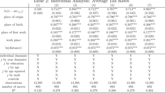
Then, we turn to an individual level analysis that studies whether individuals are more likely to select low-tax regions, conditional on moving. Our empirical choice model exploits individual variation in tax rates across the fifteen Spanish regions; given we exploit person-specific tax rates, our model allows us to account for region by year fixed effects and individual characteristics that are allowed to vary by region in order to capture counterfactual wages in alternative regions. This approach has the advantage of allowing us to account for fixed characteristics of the mover that are constant across alternative regions, any sorting based on characteristics, as well as for other policy changes that affect all individuals in the top of the income distribution. A one percent increase in the net of tax rate for a region relative to others increases the probability of moving to that region by 1.7 percentage points. Although many things may matter for decisions on where to move, taxes appear to be important. These estimates suggest that the 0.75 percentage point average tax rate differential between Madrid and Catalu˜na in 2013 increases the probability of moving to Madrid by 2.25 percentage points. This analysis is summarized in figure 1, which shows no correlation in the pre-reform period, but a strong correlation in the post-reform period for location choices and taxes.
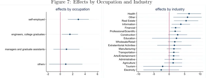
We then exploit the administrative data on occupation and industry to show that taxes play a stronger role for certain occupations and industries. Testing for
hetero-geneity across occupation and industry helps to inform the recent policy debate on the efficiency of tax schemes for top earners in specific occupations. Several OECD countries have preferential tax schemes for foreigners in high-income occupations.6 By focusing
on the heterogeneity by occupation and industry, we can shed light on the efficiency of these tax schemes. First, we replicate the result in the prior literature for scientists and find that those in the “professional/scientific” and “health” industry have large and sig-nificant migration effects; entertainers including athletes have insigsig-nificant effects, likely due to sample size. Then, we look at other occupations and industries to determine if the estimates for the occupations studied in the prior literature generalize. Our results indicate that self-employed (a self-employed individual will only have income in the data for formal contracts with firms registered with the Social Security administration) and “higher-ability” occupations are more sensitive to taxes. Our industry-level data demon-strates substantial heterogeneity with the largest effects emerging in finance, real estate, and information, in addition to the professional/scientific industries studied previously.
Our analysis comes with a caveat: our data do not allow us to disentangle a real move from a fraudulent move where the taxpayer changes residence to a second home without actually changing where they spend the majority of the tax year. In so much as this is possible, the presence of such evasion implies that mobility includes both real responses as well as tax evasion responses. From a tax revenue perspective, it does not matter if the move is a real response or simple misreporting; from a labor supply perspective, real moves may be more important.
As noted in Saez et al. (2012), absent both classic and fiscal externalities, the elasticity of taxable income (ETI) suggests that the revenue maximizing tax rate on top incomes may be as high as 80% with a broad income tax base. However, changes resulting from mobility across regions are not generally captured in these estimates and therefore understanding mobility has important implications for understanding the optimal top
6For example, Denmark has income tax exceptions for foreign scientists, Korea has exceptions for
high-tech fields, Poland has exceptions for workers engaged in artistic, scientific, sport or expert activities, and Switzerland has exceptions for managers and specialists. In the United States, many states have aggressively passed “jock taxes” that target professional athletes, which enforce tax collections based on the number of duty days worked in a state.
income tax rate. In order to interpret the elasticities that we estimate, we simulate a revenue maximization model incorporating migration. The model suggests that the effect of changes in taxes on revenue can be decomposed into a mechanical (tax rate) effect from higher taxes, a behavioral effect from changes in taxable income, and a migration effect. The last effect depends on the stock elasticity of migration. Using our stock elasticities, we find the mechanical effect dominates the other effects for all regions in Spain, which has important implications for how much additional revenue a region can raise [lose] by raising [lowering] its top tax rates. For the region of Madrid, its lower rate relative to the central government tax rate in 2014 results in revenue falling by 50 million Euro due to the mechanical effect of the lower tax rate. Using our mobility estimates, migration effects only contribute 9 million Euro more in revenue. For behavioral responses to entirely offset the mechanical effect net of mobility effects, the elasticity of taxable income would need to be 1.40, which is well above reasonable estimates of it. We conclude that, at least in the short-run, migration does not pose a large threat to redistributive taxation.
1
Institutional Details
Spain consists of 17 autonomous communities (in Spanish: comunidades aut´onomas) which are comparable to states or regions in other countries. The autonomous commu-nities are governed according to the Spanish constitution. Furthermore, the individual competences which each region assumes are regulated by a region specific organic law, known as Statute of Autonomy.7 Important for our purpose is that taxes are due at the place of residence (residencia habitual), which is declared in the local municipality of residence. Since 1994, the regions receive a share of the Personal Income Tax (Impuesto
sobre la Renta de las Personas F´ısicas) as part of their revenues, but it was only in 1997
that partial autonomy over marginal tax rates was delegated to the regions (see Dur´an and Esteller 2005). Initial regional autonomy was quite limited as regional level marginal tax rates applied only to 15% of the tax base and thus autonomous communities had lit-tle interest in changing marginal tax rates. Instead, they focused on setting tax credits, mostly for housing and renting as well as some personal circumstances such as ascendants
and decedents.8 In 2007, following some reforms, the regional-level individual tax rates
still had to complement the common tax brackets set by the central level, but they were applied to a larger share (35%) of their residents tax base.9 Therefore, in 2007, Madrid
was the first autonomous community which changed marginal tax rates, followed by La Rioja and Valencia in 2008. These regions implemented top marginal tax rates which were slightly lower (less than 0.1 percentage point) than the federal tax schedule. Murcia followed in 2009, but returned to the common federal scheme thereafter. These initial reforms resulted in very small differences in taxes across regions.
Another major wave of decentralization reforms followed this process in 2009 (last laws approved in July 2010) but regions could not exercise their new rights until 2011. Regions could now keep the revenues collected from half of the entire tax base in their territory. In addition, regions were also given the right to introduce new tax brackets on top of those implemented by the central government. In 2011, with both the ability to construct new brackets and marginal tax rates in hand along with added incentives to retain more of the tax revenue, several regions increased marginal tax rates substantially, while the ones which decreased them previously lowered their rates (Bosch 2010).10
An-other reason for the immediate reaction of regional governments was that in 2011, the federal government raised marginal tax rates substantially and regions used this event to increase simultaneously their own tax rates, or decrease them to counteract the federal increase. In subsequent years, some further changes in regional top tax brackets were implemented, but the pattern of high versus low-tax regions as of 2011 generally persists to the end of our sample in 2014.11
8Dur´an and Esteller (2006) show that those tax credits lower predominantly the effective tax burden
for the poor, as many of them fade out with income. A prominent example are tax credits given to young individuals renting a flat in various regions. However, only young and low income individuals are eligible (for example below 35 years of age and 19,000 Euros in Extremadura, and 32 years and 20,000 in Catalu˜na). Madrid allows for a small deduction of school books for families with a tax base below 30,000 Euros, to give a further example of these types of deductions.
9c.f. Ley 35/2006, de 28 de noviembre, del Impuesto sobre la Renta de las Personas F´ısicas y de
modificaci´on parcial de las leyes de los Impuestos sobre Sociedades, sobre la Renta de no Residentes y sobre el Patrimonio.
10In all subsequent discussion referring to the tax reform, we mean this 2011 reform. Any differences
prior to this reform were trivial – for top earners – in comparison.
11A confounding factor could be the re-introduction of the wealth tax at the end of 2011. The decision
was taken at the end of 2011, such that an immediate response in that year – and even one in 2012 is unlikely to happen. Further, the tax has been introduced as an explicitly temporary measure to reduce
The regional tax changes are salient to top taxpayers. Tax forms compute an individual’s average regional and federal tax liability separately so that the individual sees both average tax rates.12 When filing taxes in April, taxpayers are asked to state
their place of residence. A change of their address can be done online at the same page where individuals submit their tax declaration and becomes effective immediately.13
In Spain, the personal income tax is a dual tax which separates the income tax base and the capital income tax base. The reformonly allowed regions to alter marginal tax rates of the labor income tax base, while the capital income tax base remained taxed under a common tax schedule. Given that we will use Social Security data to study migration, pure rentiers (individuals with capital income only) will be absent from the data. However, given that these rentiers face a common federal tax rate on capital income, the decentralization of the labor income tax base is irreverent for these individuals. The reform did not affect corporate taxes, so we do not have to worry about any correlation with corporate taxes, which remain the authority of the federal government.
1.1
Descriptive Figures of the Reforms
In 2010, all regions in our data set have tax rates that are within 0.10 percentage points of each other. But, by 2014, substantial spatial variation had emerged. All tax rates increased over time in levels – although some decreased relative to the federal rate, which was changing over time. Figure 2 shows the changes for all regions and for all brackets. In order to ease interpretation, we show the tax changes relative to what the tax rate would be if the region had simply adopted the federal tax rates in that year. Relative to this standard, some regions decreased their tax rates while others increased their tax rates. Immediately following the reform, top tax rates diverged by 5 percentage points. This pattern persisted with some changes to lower bracket tax rates.
Given that many tax brackets change (and not just the top marginal tax brackets), fiscal problems during the Great Recession. Not until the end of 2012 did the government announced that the tax will also be applied in the following year, again without establishing the tax permanently.
12Although individuals know their average tax rate in the region of residence, it is unlikely they would
know the exact average tax rate in all of the alternative regions within Spain. For this reason, high-income taxpayers may use the top marginal tax rate as a proxy for their expected tax liabilities in other regions. Gideon (2017) shows that many people think that all income is taxed at the marginal tax rate.
13We do not observe the location declared on the return. However, tax inspectors afterwards might
we need to justify our focus on the top of the income distribution. The red vertical line in figure 2 shows the cutoff for the top 1% of income. Notice that the top 1% – incomes above 90,000 Euro approximately — experienced the largest changes in tax rates across regions. The tax differences for individuals even in the top 2 to 5% were relatively small across regions – this is because even if marginal tax rates differed across regions, average tax rates were relatively similar.
1.2
Who Changes By Larger Amounts?
Regions that raise their tax rates by the largest amounts might be those regions where the mobility of top earners has been declining or where the stock of top earners is large or small. Regions had little information about how individuals would respond to tax changes given the immediate decentralization and tax changes following the reform. Sim-ple correlations in appendix A.1 show that characteristics of the region related to the top 1% seem to have small effects on the tax changes. Larger correlates with the tax changes are political associations, debt, and income conditions.
Although the equilibrium tax rates may be a result of a rather arbitrary political process, this is not to say that the resulting equilibrium tax rates are as good as random. In particular, the resulting tax rates following the policy decentralization may be a func-tion of unobservable characteristics. While this is not something that we can rule out entirely, we provide evidence that this does not appear to be the case. First, we do not find pre-trends in the populations of the regions; changes in the population stocks occur after the tax changes. Second, we show that post-reform tax rate changes do not predict pre-reform populations or migration flows suggesting that regions do not set taxes based on pre-reform characteristics. Of course, other unobservable changes in state policy or state shocks may exist. While we cannot rule this possibility out with aggregate data, we then turn to individual level data where we can control for state by year shocks.
2
Description of Data
We use panel data from 2005-2014 from Spain’s Continuous Sample of Employment Histo-ries (Muestra Continua de Vidas Laborales, MCVL). The data is provided by the Ministry of Employment and Social Security(Ministerio de Empleo y Seguridad Social). This
ad-ministrative data matches individual microdata from social security records with data from the tax administration (Agencia Tributaria, AEAT), and official population register data (Padr´on Continuo) from the Spanish National Statistical Office (INE).14 The
So-cial Security administration publicly releases an approximately 4% non-stratified random sample (over 1 million observations each year) of the population of individuals which had any relationship with Spain’s Social Security system in a given year due to work, receiv-ing unemployment benefits, or receivreceiv-ing a pension. These data have been previously in applied work on labor and urban economics (Bonhomme and Hospido 2017; De la Roca and Puga 2017). Individuals from Navarre and the Basque Country do not appear in the data because these regions operate independent fiscal systems.15 If an individual is
in the data, they remain in the data as long as they have contact with the Social Se-curity ministry, but new observations enter each year so that it remains representative. Self-employed individuals that make contact with the Social Security system do appear in our data, however, we only observe income for them if they have a relationship with a registered firm, as the firm remits taxes on their behalf. Self-employed individuals that do not have contracts with firms do not appear in the data; however, we believe that at the very top of the income distribution most self-employed individuals provide services to firms such that they will be covered in our sample. Nonetheless, even for self-employed individuals with some contracts with firms, we may mismeasure their true income.
One key is that from 2005 to 2014, the Social Security data are matched to income from tax data. These income tax data are valuable because they are not subject to censoring; Social Security contributions are censored and do not contain some portions of income that are important for high income tax payers. Given we will focus on top income taxpayers it is important we have income data that is not censored and contains all sources of income.16 The observational unit of the raw data is based on each contact 14Residence data in the Social Security data are less controversial; the tax return data often reports
the location of work. Social Security data contains residence information based off local registers.
15We exclude the individuals living there from our analysis. We treat people moving to those two
regions as people leaving the sample for any other reason (moving abroad, etc.). However, we do include people moving from those two regions to another region in Spain as we observe their income in the new destination and know the origin from the social security database. We furthermore exclude Ceuta and Melilla, two autonomous cities (not autonomous communities) on continental Africa.
(for example, job) an individual had within a given year with Social Security. We define the main work affiliation in each year as the one which was active for the longest time span since starting work. We aggregate this data at the individual level to obtain a panel data set which sums all individual income sources in a given year for a given tax payer.17
We define a change of location if an individual changed his or her residence between t and t−1.18 Residence data of the current year is updated using the residence of April int+ 1, which ensures that this period overlaps with the tax year as tax declarations are due in April to June. As an example, an individual would be characterized as a mover in 2012 if he was living in a different region between April 2012 and April 2013 compared to his residence between April of 2011 and April 2012. In this way, his 2012 income is the relevant one for tax purposed in the region he moved to.19 While residence information
is available at much smaller spatial units, in this paper, we will define a “mover” as an individual that relocatesacross (not within) regions. One reason for this is that we only observe municipality codes for individuals living in sufficiently large cities, which means that many within region moves remain unobserved to us.
We construct taxes using the sum of all reported income by different employers within each year which is subject to the personal income tax (labor income, reported self-employed income, and income in-kind). Given this information and other attributes, we simulate average and marginal tax rates for each individual in each year for each region travel and other expenses, and dismissal compensations. These differences seem more relevant for high skilled workers as the correlation in levels between contributions and taxable labor income is lower for the first group [high-skilled] (70%) than for the others (over 85%).” Given our focus on high-income taxpayers we use the tax income data.
17Only a small fraction of the sample are reported as “married” with a substantial fraction declaring
“other.” Because of this, two individuals may move in our data when they are a common household. Our results are robust to using only county pairs featuring only a single mover in a given year.
18The transition matrix of movers in the pre- and post-reform period are given in appendix A.2. 19Registration is mandatory within three month and municipalities have an incentive to register citizens
because they receive transfers allocated on a per capita base (Foremny et al. 2017). An alternative location variable which is available in this data-set are the region the firm provides when they remit taxes for the individual. This does not have any legal effect on tax declarations (it is not the state the individual files their taxes in), but rather corresponds to the address on file with the employer reporting the contract. We observe 57% of movers have firms reporting the same state from the registrar data. Adding the observations for which the province declared by a firm coincides with the residential province before moving increases the share to 96%. This indicates that there is rather a lag of updating the firm database than the official register, which is not surprising given that the address communicated to the firm does not have any legal (or even tax) consequences. Thus, the registrar data is preferred. However, we reestimate our individual model excluding observations where the firms report a different address than the location before or after the move in the registrar data; results remain similar.
using the information in the tax code provided by official documents.20 This simulation
takes into account the variation of marginal tax rates, their brackets, and basic deductions and tax credits for ascendants, decedents, and disabilities. We do not take into account any further region specific deductions or tax credits. However, given that we focus on high income individuals, this would almost never affect the marginal tax rate and the average tax rate only to a negligible amount as those omitted policies are targeted to low income individuals.21 We use the tax calculator to simulate the tax rate in the region of residence and the tax rates in all counterfactual alternative regions.
Summary statistics of our data are given in appendix A.4. Unique to our set-ting is detailed data on occupation and industry. The appendix also shows descriptives concerning the top occupations and industries of movers in the top 1%.
3
Aggregate Analysis
3.1
Theory of Population Stocks
For simplicity, consider a two region economy where r = o, d indexes the two regions, which we call origin and destination for simplicity.22 The utility of top income individuals
living in regionr in period t is given by:
Vr,t =αu(cr,t) +πv(gr,t) +µr−γρ(Nr,t) (1)
wherecr,t is private consumption of the individual,gr,tis public services consumption, µr
is the value of other amenities that are specific to living in the region. The function ρ is a disutility that depends on population. The ρ(Nr,t) function allows us to indirectly
bring in housing markets into the problem: a region becomes less attractive, the larger is its population perhaps because housing prices increase. In particular, fewer people in a region mean the cost of housing will be lower which raises utility relative to a region
20We use the tax laws to write a tax calculator for Spain similar in spirit to TAXSIM. Details of the
calculator are in appendix A.3.
21Omissions from the tax calculator are common to all calculators. Even NBER’s TAXSIM does not
present a complete set of tax rules for all states and years. Measurement error is addressed via IV.
22For lack of a better term, we refer to one regiondas the destination and the othero as the origin.
Given these are stocks and not flows there is no origin or destination per se. Nonetheless, this verbiage will help us talk about the model without having to refer to arbitrary region pairs.
with more people and higher housing costs.23 In particular, this congestion cost it is an
alternative mechanism to get to a spatial equilibrium even without formally modeling housing price adjustments. Following the standard in the literature, we assume that the separable functions u, v, and ρeach take on the log functional form.
Each individual supplies a fixed unit of labor so that given the nature of the problem, an agent consumes all after-tax income: cr,t = (1−τr,t)wr,t where τr,t is the
tax rate on wages wr,t. In practice, τr,t is not a single rate but rather is the average tax
rate on wages. If the tax system exhibits any progressivity, then τr,t will be a function
of wr,t; thus, a progressive tax system would require estimation to use an average tax
rate. To see this, a progressive tax system would be given by the tax function T(wr,t)
and so consumption would be cr,t = wr,t −T(wr,t) = (1−atrr,t)wr,t and the subsequent
derivation follows using an average tax rate.
To close the model, we assume a simple model of production. Production in any given region is given byf(Nr,t) and satisfies the standard propertiesfNr,t >0 andfNr,t <
0; the price of output is normalized to one Euro. With mobility, the equilibrium in the labor market requires the wage rate equal the marginal product of laborwr,t =fNr,t(Nr,t).
Assuming that production is given byArNr,tθ K¯rϑwhere Ar are fixed productive amenities
in the region and ¯Kr is the land/capital stock that is fixed in the short run.24 Then we
have in eachr that wr,t = ArK¯rϑ
Nθ
r,t .
A locational equilibrium requires for all r = o, d that Vo,t = Vd,t = V. Setting
Vo,t =Vd,t, taking logs of the equilibrium wage equation and substituting implies
ln(Nd,t No,t ) = 1 θ+αγln 1−τd,t 1−τo,t + π α(θ+αγ)ln gd,t go,t +ζd−ζo (2)
where ζo and ζd are defined to include the fixed productive amenities, fixed capital
re-sources and consumption amenities across regions defined above. The above equation
23To see the idea of this function, consider an example. Suppose both regions were ex ante identical and
private and public consumption are the same in both regions. Then an individual who moves from region
o todwill, all else equal, realize a lower level of utility in regiondbecause after the moveNd,t > No,t.
For this reason, we think this is an attachment to home function.
characterizes the equilibrium in the model.25 Notice that the endogenous adjustment of
wages can be obtained as dlndln(1(w−r,t)τr,t) = dlndln(1(N−τr,t)r,t) × dlndln((Nwr,t)r,t) =−θθ+1γ α
, which allows for the possibility of less than full capitalization of wages. This expression clearly highlights the role of the congestion cost and the parameter γ.
3.2
Methods
We estimate the pairwiseequilibrium condition derived in (2). Denote the net of tax rate with respect to the average tax rate by 1−atrd,t [1−atro,t] in the destination [origin]
region. We calculate the average tax rate for a representative taxpayer in the top 1% of the income distribution. We estimate for the working-age population:
ln(Nd,t No,t
) =β[ln(1−atrd,t)−ln(1−atro,t)] +ζd+ζo+ζt+δln
gd,t
go,t
+Xdo,tφ+εdo,t (3)
where β captures the effect of taxes on population stocks, which is a function of the structural parameters in (2).26 As suggested by theory, we include origin fixed effects that capture amenities (both for households and firms) in the region of origin and des-tination fixed effects that capture such amenities in the desdes-tination region. These fixed effects also capture any time invariant policies of the regions over our sample. Time fixed effects are included in the model to capture any aggregate shocks. As suggested in (2), we control for region-level spending changes across the regions. These spending controls are designed to capture the effect of any changes in services that may make a region more attractive following a tax change. In particular, we control for differentials on basic public services, social protection programs, public programs, general spending, and transportation infrastructure. In some specifications we include a vectorXdo,t, where
we control for time varying, region-pair specific shocks including economic shocks, demo-graphic shocks, and regional amenities. These controls help facilitate identification given that the tax changes are not likely random. Given the set of fixed effects and covariates,
25The model can be derived without theρfunction using a fixed cost of moving by lowering utility in the
destination region by that fixed cost. In this case, the only difference is the degree of capitalization into wages. Our model delivers partial capitalization into wages. The fixed cost delivers full capitalization.
26Note, as discussed previously, there were some very small tax differentials (around 0.10 percentage
points) that existed prior to 2011. For ease of interpretation, we set these differentials to zero prior to 2011. If we include them, the coefficient is almost unchanged.
identification requires that, absent tax changes, region-pair stocks are fixed over time. Notice (2) leads to a structural interpretation of the estimated coefficient in the locational equilibrium: β is the effect of tax rate changes including their indirect effects through changes in the regional wages, i.e. the effect taking all fixed regional character-istics (amenities) and public services as given except for tax rates and wages.27 Given the structural interpretation ofβ,the endogenous capitalization into wages does not pose a threat to identification, but other unobservable wage shocks that are correlated with tax changes would be problematic. To deal with other shocks to wages, we control for time-varying regional economic conditions in Xdo,t.
Theory implies to estimate the equilibrium condition using the ratios of popula-tions and taxes rather than the level of the region’s own population. In particular, this pairwise ratio is useful because we have a small number of regions, which implies the number of people in a given region depends on the entire vector of net of tax rates in all of the regions. Thus, tax changes in regionr0 6=r will have anon-zero effect onNr,t. This
is a purpose of estimating the stocks in pairwise ratios. Of course, this pairwise estima-tion complicates treatment of the standard errors and interpretaestima-tion ofβ. We cluster the standard errors three ways to account for correlation over time within region-pairs and to account for the correlation of errors within both origin and destination by year pairs. Estimating the location equilibrium condition in ratios influences the interpreta-tion of β. Given we allow the tax rate of a given region to influence the population of other regions, the estimating equation delivers the elasticity of the ratios, Nd,t/No,t.
Differentiating (3) with respect to the net of tax rate in regiond, yields:
β = dln(Nd,t) dln(1−atrd,t)
− dln(No,t)
dln(1−atrd,t)
≡η−µ (4)
where η is the stock elasticity of the population in region d with respect to its own net-of-tax rate andµis the cross-elasticity of region o’s population with respect to regiond’s
27A similar estimating can also be derived from a stochastic McFadden-type location choice model
without assuming spatial equilibrium through wages. But, then (endogenous) wages would need to be controlled for in its estimation. This is an important contribution of the theory because dealing with endogenous wages would be difficult.
net-of tax rate. Given η > 0 and µ < 0 are opposite signed, we can conclude that our estimate of β will over-estimate the elasticity of the stock of a given region. However, as the number of regions becomes large, then µ → 0. In our setting, with fifteen regions, we expect µ to be non-zero, but relatively close to zero and thus β acts as a reasonable approximation to the stock elasticity. We verify this is true by estimating the model in levels, which assumes a large number of regions and zero cross-price effects.
Some notes concerning the empirical model are in order. First, in our baseline specifications, we utilize net-of-average tax rates. To construct the average tax rate, following Moretti and Wilson (2017), we simulate taxes in all years and regions for a representative taxpayer in the top 1% holding fixed (across regions and time) income and any inputs to our tax calculator so that variation in the rate is only due to statutory changes. As noted above, the use of the average tax rate is theoretically grounded. However, some of the prior literature has presented results using the top marginal tax rate (Kleven et al. 2013; Akcigitet al.2016) as a good approximation of the average tax rate. We also present results using the top marginal tax rate in each region, but note it is not a good approximation to the average tax rate in our setting. The top marginal tax rate will be correlated with the average tax rate because regions that raised the top tax rate were also generally regions that raised rates in lower income brackets (see figure 2). Although our preferred specification uses the (theoretically grounded) average tax rate, the top marginal tax rate may be very salient when determining the tax liability of the alternative regions; although individuals know the average tax rate in their region, they are unlikely to be able to calculate this across all of the alternative regions.
We estimate a stock model rather than a flow model. First, the stock elasticity is the parameter of interest in the revenue simulations we will conduct. Second, estimation in the flow model raises selection concerns because we do not observe migration between some regions due to our 4% sample and because a flow model would miss international migration and to the Basque country and Navarre; the stock model will not. Finally, a flow model would rely on a model where utility of being in any location is always conditional on where individuals are located to start with in periodt; then identification requires
region-pair migration flows are fixed over time rather than the stocks. Appendix A.5 discusses this in detail. The stock model avoids all of these issues and in our opinion, provides a more accurate measure of all tax-induced migration. Limitations of the aggregate analysis resulting from non-random setting of tax rates are addressed in section 4 where we control for time varying region-specific shocks.
3.3
Results
Given the simple panel data setting, we present our baseline results visually. To do this, we regress the stock ratio on the fixed effects and controls and then predict the residuals. We then regress the net of average tax rate variable on the fixed effects and predict the residuals. We then bin the residuals into equally sized bins and fit a line of best fit through these data. Figure 3 shows the baseline results; the upper two panels present the results using the average tax rate while the lower panel shows the marginal tax rate. We present all results with and without covariates to see if our identifying assumption is reasonable. Because all tax variables are in terms of the net of tax rate, when individuals keep more on the Euro in regiondrelative to regiono, they are more likely to move to (or stay in) regiond and the stock increases in d relative to o. As the net of tax differential increases, we see that it is consistent with β > 0. The addition of covariates does not meaningfully change the slope, but does reduce the noise. The bottom panel shows the regression using the marginal tax rate. Although the vertical axis is identical to the upper panel, the horizontal axis is more disperse because differences in top marginal tax rates are larger than average tax rates. Thus, the slope of the line of best fit remains positive but is flatter because a one percent change in the net of (marginal) tax rate will have a smaller effect on changing tax liability.
We present point estimates of β and standard errors for the aggregate analysis in table 1. If we assume that the cross-elasticity is small, the specification without controls suggests the stock elasticity is approximately 0.92. Our estimates of the elasticity are stable and are not statistically different with or without other covariates. With covariates, it rises just above unity. This estimate of the elasticity is higher than the estimates in Moretti and Wilson (2017), who obtain a stock elasticity of 0.45; Akcigit et al. (2016)
estimate an elasticity of 1 for foreign star scientists. It is larger than Young et al.(2016) who find very small effects. The elasticity with respect to the top marginal net-of-tax rate is 0.65; the smaller elasticity makes intuitive sense because a change in the top marginal tax rate only affects some taxpayers.
A concern with this model is that we may overestimate the stock elasticity re-sulting from migration because of taxable income responses. In particular, we might worry that in regions lowering their tax rates, taxable income may rise resulting in more people moving into the top 1% of the income distribution in that region. To address this concern, we implement several robustness checks. In table 1 we show the results are robust to controlling for the (endogenous) ratio of taxable income reported by the top 1% in the region pairs. Second, and more preferably, we also adjust the population stocks accounting for movement within the income distribution. Let ∆r,t be the number
of people who move in/out of the top percentile of the income distribution in region r. This number is calculated as the number of people who are in the top 1% this year but were not in it last year minus the number of people who were in the top 1% last year but are not this year. Then we calculate an adjusted stock ratio using Ngr,t=Nr,t−∆r,t. We
then run all specifications using ln(Ngd,t/Ngo,t) as the dependent variable so that we are
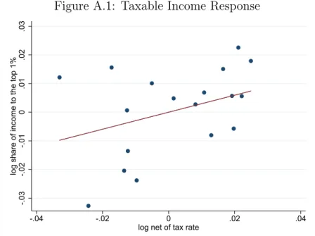
exploiting variation in the stock of people in the top 1% adjusted for any yearly churn in the income distribution. After doing this, with covariates, we estimate an elasticity of 0.88, which falls slightly suggesting our prior estimates may capture some taxable income responses.28 We also estimate a taxable income elasticity directly by regressing the share of total earned income (working age individuals, excluding pensions and unemployment benefits) in a region earned by the one percent on the net of tax rate, region and year fixed effects. This regression estimates a small insignificant elasticity suggesting we are identifying mobility effects in our stock analysis. Appendix A.6 shows the small taxable
28Again, assuming the cross-elasticity is small, to interpret the economic magnitude of the 0.88
elas-ticity in column 4, the average region in our sample has a stock of 565 taxpayers in the top 1% of the income distribution (recall we have 4% random sample, so multiplying by 25 yields population level estimates). The average net of tax rate (federal plus state) implies that a 1% change in the net of tax rate results in a 0.54 percentage point change. The absolute value of the net of tax differential between regions is on average 1.2 percentage points or 2 times a 1% change in regional tax rates. Combined with our elasticity, this implies a change in the stock of top taxpayers by 11 taxpayers.
income response. This is consistent with Rubolino and Waldenstr¨om (2017), which esti-mates a taxable income elasticity for the top percentile in Spain of 0.05. The results of these exercises suggest that we are not identifying taxable income responses. However, to further address this issue, we will subsequently turn to an individual analysis where taxable income responses will not be a concern for identification.
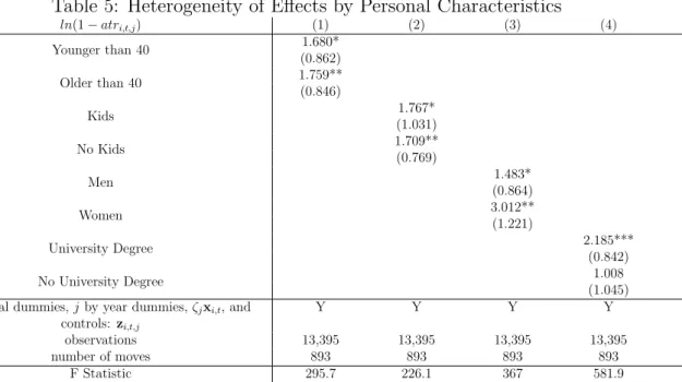
We also test for a heterogeneous effect of the tax reform on other lower income groups. In particular, we consider whether these lower income groups respond to the average tax rate for top income taxpayers. In figure 4 we present (using the same scale as the upper panel in the prior figure) results for the top 5% (excluding the top 1%) and the top 10% to 5% of the income distribution. A mildly positive pattern emerges in response to the average tax rate differentials for the top 5% and the slope is declining as income declines. So, what makes lower income households less responsive to the tax differentials? They have smaller tax rate differentials due to progressivity and the top 1% average tax rates may not be relevant for them unless they anticipate income growth, they may care relatively less about tax rates and more about public services because of non-homothetic preferences, or they may have lower moving probabilities because of relatively higher moving costs and less job opportunities. Thus, these results should be interpreted as an analysis of heterogeneity rather than a placebo test given that the differences along these dimensions cannot be ruled out.
Given identification is based on a large reform, we wish to show a break in the patterns following the 2011 reform. For each region pair d and o, if the net of tax differential increases in region d relative to region o, we classify that pair as one where the net of tax rate increases. The left panel in figure 5 shows the raw averages of the stock ratio for pairs where the region d gets to keep more income (taxes fall) relative to region o. For these observations, the stock ratio increases following the reform and remains higher. To do this formally, we implement an event study approach by estimating
ln(Nd,t No,t ) =ln(1−atrd 1−atro )[ −2 X y=−6 πy1(t−t∗ =y) + 3 X y=0
γy1(t−t∗ =y)] +ζo+ζd+ζt+Xod,tφ+εdo,t
where ln(1−atrd
1−atro) is the average log differential of the net of tax rates in the post-reform
years. Then, 1(t−t∗ = y) are indicator variables relating to the time since the reform happened in t∗ = 2011. As such, πy show the evolution of the stock ratios prior to the
reform and the γy show the evolution following the reform. Multiplying by ln(11−−atratrdo)
captures the intensity of the treatment and allows us to jointly estimate the effect of relative increases and decreases in one specification. The right panel of figure 5 shows no clear pre-trends – if anything, a slight downward trend – but an immediate level increase in the stock ratio following the reform; given the large jump on impact this may suggest tax evasion rather than real moves. The regions that lowered rates allowing residents to keep more, saw an immediate increase in the stock of top income taxpayers. To reduce noise in the post-reform period, the generalized event study design can also be presented as a simple dif-in-dif controlling for trends; the results are given in appendix A.6. The event study is reassuring because population changes do not pre-date the tax reform.
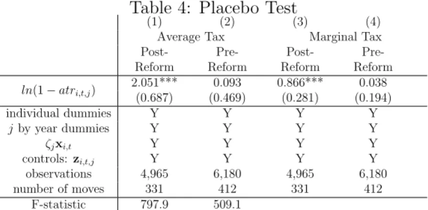
Finally, we conduct an exercise in the spirit of a placebo test using the pre-reform period. To do this, we take our measured tax differentials from 2011-2014 and lag them into the pre-reform period. We then match these post-reform tax rates to the years prior to the reform. We show in figure 6 that no significant correlation between the pre-reform stock ratio changes of the top 1% and post-reform tax rate changes exists. Nonetheless, the aggregate analysis cannot rule out confounding unobservables and potential taxable income responses. For this reason, we subsequently exploit individual data to control for all time varying regional characteristics and have proxies for counterfactual incomes.
4
Individual Analysis: Where to Move?
4.1
Methods and Identification
Although the aggregate analysis is appealing in its simplicity, we cannot rule out the possibility of unobservable time-varying region-specific covariates that are correlated with taxes and populations, i.e. although the tax rates may have come about from a random political process, the tax rates may not be random. To address this concern, we now use data for an individual tax-payer i who moves in year t. An individual enters the sample if the individual is in the top 1% in year t and relocates across regions between
t and t−1 (and only is in the sample in the year of move). Moves within a region are not included in our sample; we do not include these moves because some regions are composed of a small number of (or a single) provinces and we cannot observe moves if they are within the same province unless a municipality code is available. We only observe municipality codes for individuals living in sufficiently large cities and therefore do not use this information.29 Subsequently, we will refer to an individual that moves regions as a “mover”. We denote the alternative residential options (different regions within Spain) as j in our model. In particular, we focus on working-age movers in our estimating sample from 2006 to 2014; the vast majority of individuals move only once over the course of our sample but some individuals move multiple times in which case they appear in our data multiple times. For most individuals there will only be one time observation (but still J region observations). A “move” is a time-specific move which is indexed by (i, t) and the choice set for each move is indexed by j. One justification for focusing on movers is that local tax rates are likely a function of all individuals’ location decisions. Because movers are a relatively small share of the population of a given region, it is likely that the equilibrium tax rates selected following the fiscal decentralization are driven by the large share of the stayers – reducing endogeneity concerns (Schmidheiny 2006; Br¨ulhart et al. 2015). In addition, as noted in Schmidheiny (2006), “Households do not daily decide upon their place of residence. There are specific moments in any individual’s life [first job, family changes, career opportunities] when the decision about where to live becomes urgent.... Limiting the analysis to moving households therefore eliminates the bias when including households that stay in a per se sub-optimal location because of high monetary and psychological costs of moving. However, the limitation to moving households introduces a potential selection bias when the unobserved individual factors that trigger the decision to move are correlated with the unobserved individual taste for certain locations.”
Focusing on movers leaves us with a sample of 893 moves in the top 1%, of which
29Thus, our analysis uses a particular type of mover: those that move regions. Although data
limita-tions are an important reason to focus on this type of move, this sample selection would be justified if tax differentials are important for individuals changing the labor market or region rather than changing houses within the same region.
approximately 330 are in the post-reform period, resulting in 13,395 move-region obser-vations in our dataset. Focusing on movers may raise selection concerns, which could be addressed if we followed the approach of Moretti and Wilson (2017) to model the moving decision and the decision of where to move in a unified framework. The aggregate analysis discusses reasons why we elect not to follow this approach. Note that the aggregate stock analysis allowed “stayers” and “moving” residents to respond to taxes; in this section we study the effect of taxes conditional on moving regions. In appendix A.7, we also present results for the full sample of movers and stayers; the appendix also tests for differences in the characteristics of movers and stayers and finds no significant difference in average incomes prior to the move.
The dependent variable di,t,j is coded one for the chosen region of residence for a
given move (i, t) and zero for all other region that are not selected. In its most complex form, we estimate the following linear probability model where the person-specific tax rates from our tax calculator are denoted byτi,t,j:
di,t,j =βln(1−τi,t,j) +αi,t+ιt,j +ζjxi,t+γzi,t,j +εi,t,j. (6)
Because we use moves pre- and post-reform, and because all taxes for a given individual are the same in the pre-reform period, the pre-reform period helps us to pin down other explanatory variables.30 Our model contains individual move dummies denoted α
i,t,
al-ternative region by year dummies ιt,j, individual characteristics interacted with region
dummies ζjxi,t, and move specific covariates that vary across the choice regionszi,t,j. We
will discuss each of these components in turn.
Following Bertoniet al.(2015), we estimate our model using a linear model rather than a McFadden-type conditional logit model. Given we have elected to utilize a linear model, we wish to highlight two important properties. First, predicted choice probabilities over all regions will add up to 1 for an individuali moving in yeart. Second, an increase in the tax rate in one region does theoretically increase the probability of choosing this
30In all that follows, the very small tax differentials in the pre-reform period are not utilized. Including
region while it decreases the probability of choosing any other region. Along both of these points, the presence of a fixed effect αi,t for each move is critical because it forces the
predicted probabilities to sum to one and therefore an increase in one region will lower the probability of the alternative regions; intuitively, this fixed effect adjusts the predicted probability from all other covariates by capturing the average deviation from the average probability.31 However, the predicted probability of a mover selecting any one region need not be bounded between zero and one; even with this, the predicted probabilities across the choice regions will sum to one. The inclusion of αi,t also forces identification
of our parameter of interest to come from variation in tax rates across regions for a given move. In this way, we exploit the income tax differential across regions for a given tax payer which relocated. In the subsequent paragraphs, we discuss each of the components of this regression.32
Taxes. The theoretically appropriate tax rate, the “true-ATR”, would be the
actual effective average tax rate facing a given individual in a given region, which is a function of the individual’s (possibly counterfactual) income in that region and the tax system in that region. Because this counterfactual is not observable to us, we use a “simulated-ATR” measure, which is the average tax rate for a given income level in a given region; this simulated tax rate is a function of the (assumed to be constant) income
31For ease of notation, we prove this for an equation with a single covariate denoted byx
i,t,j, the sum
of the predicted probabilities for a given move (i, t) from our regression is given by
P
j(βxb i,t,j+dαi,t) = P
jβxb i,t,j+Pjdαi,t = βb·J·xi,t+J·dαi,t = J·[βxb i,t+dαi,t] (7)
where the upper-bar denotes an average over the j’s. Given we have J alternative regions and, for a given move, only one region can be chosen:
di,t=
1
J. (8)
As shown in Greene (2003), the linear model implies that the estimated fixed effects,dαi,t, are given by
d
αi,t=di,t−βxb i,t⇒di,t=βxb i,t+dαi,t. (9)
Plugging (9) into (7) and using (8), proves that P
j(βxb i,t,j+αbi) = J·di,t =J ·
1
J = 1. This, then,
necessarily implies that an increase in the probability of selecting one region must lower the probability of the alternative regions.
32Our estimation strategy of using a linear model comes with one caveat: unlike the standard
multino-mial choice model, our model assumes that the percentage point effects are constant. In other words, very small regions with very low baseline probabilities, would experience the same effect in percentage points as large regions with high baseline probabilities. However, given the inclusion of region by year fixed effects, we are controlling for characteristics like jurisdiction size that influence the baseline probabilities.
level across regions and the tax schedule in that region. In the baseline specification, the simulated net of tax rate is person-specific (not for a representative taxpayer). Specif-ically, because counterfactual wages are not observed to us, we use our tax calculator to construct the individual’s average tax rate by assuming her income is constant across the regions. However, in practice and as shown by our theory which allows for wage capitalization to arise in spatial equilibrium (recall (2)), income may differ across the re-gions. In particular, a given individual is more likely to move to a high-income region all else equal. Given that taxes are progressive, by assuming that income is constant we will overestimate counterfactual wages (because we observe them in the selected, likely higher wage, region) and therefore overestimate counterfactual tax rates. This raises measure-ment error concerns, because the average simulated tax rates depend on the assumed to be constant income across regions and not the true counterfactual wages that may differ across regions. However, as noted in Kleven et al.(2013), the (individual’s) marginal tax rate, the tax rate facing a given individual in a given region, proxies for the exogenous component of the ATR because it is independent of earnings and allows us to implement an IV strategy discussed below.33 This also has the advantage of reducing measurement
error in the average tax rate that might result from elements of the tax code not captured by our tax calculator. The variation in the marginal tax rate, across regions for the top 1% relative to other income groups is verified by looking at the within mover variation in appendix A.7. The variation across different regions a taxpayer could choose increases substantially from 2011 onward, and is much more pronounced for the top 1% of the income distribution.
Wage controls and sorting. Equilibrium wage differentials across regions may
also be important to the choice of region. Although we assume wages are equal across
re-33Unlike Klevenet al.(2013) we cannot use the top marginal tax rate as an approximation for ATR
because most individuals do not have income well into the tax bracket. Thus, we use the mover’s
marginal tax rate in the region as an instrument. In particular, consider and individual in the second highest tax bracket. For this individual we use the marginal tax rate in that bracket; we do not use the top tax rate on income. This allows us to identify our effect using individual variation in tax rates while also accounting for state by year effects. If changes in income across regions is small, the marginal rate is independent of earnings because it will not change the bracket the individual falls into. However, if changes in income across regions is large (for that person), then this may potentially result in the individual changing tax brackets. We address this issue subsequently in the paper.
gions to calculate taxes, wages may differ across regions and influence migration decisions irrespective of taxes. To control for unobservable counterfactual wages, we include loca-tion specific dummies interacted with characteristics of the mover (for example, age, age squared, male, and education). Denote the vector of characteristics interacted with region specific dummies as ζjxi,t. This allows the returns to education and the skill premium
to vary by region; by allowing observables to vary by region, these observable charac-teristics are used to account for unobservable counterfactual wages. Although motivated by wage differentials, this is a very rich parameterization that also can be interpreted as capturing any sorting of specific types of individuals to particular regions. For example, if high-educated or older individuals have a preference for locating in a particular region, this specification will capture this sorting.
Public services and regional shocks. Public services across regions matter.
The inclusion of region by year dummies (ιj,t) captures any time varying policies – such
as changes in public services – that are constant across all individuals in the top 1%. In general, however, we note that tax increases on the rich are not likely to change public services for the rich as these taxpayers are net payers into the tax system. Thus, in addition to accounting for regional policies, ιj,t also account for time-varying amenities or
economic shocks in the alternative regions that affect individuals in the top 1%. Unlike in the aggregate analysis, inclusion of these dummies is possible because we exploit mover-specific income to calculate tax rates rather than income for a representative taxpayer.
Other controls. Finally, moving costs between regions, which could be thought
of as higher γ in our theory, also matter. To capture these moving costs, we include in a vector zi,t,j a dummy variable that equals one if the region is the place of birth
for the individual. We also include a dummy variable for the region of the principle workplace of the individual and a dummy variable that equals one if the individual had their first job in that region. Following a standard gravity model of migration (Bertoni
et al.2015), we also include the log of distance between the region of prior residence and
each of the alternative regions. This captures the fact that nearby regions have lower moving costs because they allow individuals to maintain their social and family network.