Adaptive cost-sensitive online classification

(1)

Singapore Management University

Institutional Knowledge at Singapore Management University

Research Collection School Of Information Systems

School of Information Systems

2-2019

Adaptive cost-sensitive online classification

Peilin ZHAO

South China University of Technology

Yifan ZHANG

South China University of Technology

Min WU

Institute for InfoComm Research

Steven C. H. HOI

Singapore Management University, [email protected]

Mingkui TAN

South China University of Technology See next page for additional authors

DOI:

https://doi.org/10.1109/TKDE.2018.2826011

Follow this and additional works at:

https://ink.library.smu.edu.sg/sis_research

Part of the

Databases and Information Systems Commons, and the

Numerical Analysis and

Scientific Computing Commons

This Journal Article is brought to you for free and open access by the School of Information Systems at Institutional Knowledge at Singapore Management University. It has been accepted for inclusion in Research Collection School Of Information Systems by an authorized administrator of Institutional Knowledge at Singapore Management University. For more information, please [email protected].

Citation

ZHAO, Peilin; ZHANG, Yifan; WU, Min; HOI, Steven C. H.; TAN, Mingkui; and HUANG, Junzhou. Adaptive cost-sensitive online classification. (2019).IEEE Transactions on Knowledge and Data Engineering. 31, (2), 214-228. Research Collection School Of Information Systems.

(2)

Peilin ZHAO, Yifan ZHANG, Min WU, Steven C. H. HOI, Mingkui TAN, and Junzhou HUANG

This journal article is available at Institutional Knowledge at Singapore Management University:https://ink.library.smu.edu.sg/ sis_research/4036

(3)

Adaptive Cost-Sensitive Online Classification

Peilin Zhao , Yifan Zhang , Min Wu , Steven C. H. Hoi , Mingkui Tan , and Junzhou Huang

Abstract—Cost-Sensitive Online Classification has drawn extensive attention in recent years, where the main approach is to directly online optimize two well-known cost-sensitive metrics: (i) weighted sum of sensitivity and specificity and (ii) weighted misclassification cost. However, previous existing methods only considered first-order information of data stream. It is insufficient in practice, since many recent studies have proved that incorporating second-order information enhances the prediction performance of classification models. Thus, we propose a family of cost-sensitive online classification algorithms with adaptive regularization in this paper. We theoretically analyze the proposed algorithms and empirically validate their effectiveness and properties in extensive experiments. Then, for better trade off between the performance and efficiency, we further introduce the sketching technique into our algorithms, which significantly accelerates the computational speed with quite slight performance loss. Finally, we apply our algorithms to tackle several online anomaly detection tasks from real world. Promising results prove that the proposed algorithms are effective and efficient in solving cost-sensitive online classification problems in various real-world domains.

Index Terms—Cost-sensitive classification, online learning, adaptive regularization, sketching learning

Ç

1 I

NTRODUCTION

W

ITH the rapid growth of datasets, the technologies of machine learning and data mining power many respects of modern society: from content filtering to web searches on social networks, and from goods recommenda-tions to intelligent customer services on e-commerce. Gradu-ally, many real-world large-scale applications make use of a family of techniques called online learning, which has been extensively studied for many years in machine learning and data mining literatures [1], [2], [3], [4], [5], [6]. In general, online learning is a class of efficient and scalable machine learning methods, whose goal is to incrementally learn a model to make correct predictions on a stream of samples. This family of methods provides an opportunity to solve many real-world applications that data arrives sequentially while predictions must be made instantly, such as malicious URL detection [7], [29] and portfolio selection[8]. In addition, online learning is also good at solving large-scale learning tasks, e.g., learning

support vector machinefrom billions of data [9].

However, although online learning was studied widely, most existing methods were inappropriate to solve cost-sensitive classification problems, because most of them seek performance based on measurable accuracyor mistake rate,

which are obviously cost-insensitive. As a result, these algo-rithms are difficult to handle numerous real-world prob-lems, where datasets are always class-imbalanced, i.e., the mistake costs of samples are significantly different [10], [11], [12]. To solve this problem, researchers have suggested to use more meaningful metrics, such as the weighted sum

of sensitivity and specificity [13], [14], and the weighted

misclassification cost[10], [15] to replace old ones. Based on this, many batch classification algorithms are proposed to directly optimize prediction performance for cost-sensitive classification over the past decades [10], [15]. However, these batch algorithms often suffer from poor scalability and efficiency for large-scale tasks, which make them inap-propriate for online classification applications.

Although bothonline classificationandcost-sensitive classifi-cationwere studied widely, quite few literatures study cost-sensitive online classification. As results, the Cost-Sensitive Online Classification framework [16], [17] was recently proposed to fill the gap between online learning and cost-sensitive classification. According to this framework, a class of algorithms named as Cost-Sensitive Online Gradient Descend (COG) was proposed to directly optimize prede-fined cost-sensitive metrics (e.g., weighted sum or weighted misclassification cost) based on online gradient descent tech-nique. Particularly, compared with other traditional online algorithms, COG shows strong empirical performance in solving cost-sensitive online classification problems.

However, although COG is able to handle the Cost-sensitive online classification tasks, it only takes the first order information of samples (i.e., weighted mean of the gradient). It is obviously insufficient, since many recent studies[3], [18], [19], [20] have shown that comprehensive consideration with second-order information (i.e., the corre-lations between features) significantly enhances the perfor-mance of online classification.

As an attempt to remedy the limitation of first-order approaches, we propose the Adaptive Regularized P. Zhao, Y. Zhang and M. Tan are with the South China University of

Tech-nology, Guangzhou, Guangdong 510630, China. E-mail: peilinzhao@hotmail. com, [email protected], [email protected].

M. Wu is with the Institute for Infocomm Research, Singapore 138632. E-mail: [email protected].

S. C. Hoi is with Singapore Management University, Singapore 188065. E-mail: [email protected].

J. Huang is with Tencent AI Lab, Shenzhen, Guangdong, China. E-mail: [email protected].

Manuscript received 7 Dec. 2017; revised 27 Mar. 2018; accepted 30 Mar. 2018. Date of publication 12 Apr. 2018; date of current version 9 Jan. 2019. (Corresponding author: Mingkui Tan.)

Recommended for acceptance by L. B. Holder.

For information on obtaining reprints of this article, please send e-mail to: [email protected], and reference the Digital Object Identifier below.

Digital Object Identifier no. 10.1109/TKDE.2018.2826011

214 IEEE TRANSACTIONS ON KNOWLEDGE AND DATA ENGINEERING, VOL. 31, NO. 2, FEBRUARY 2019

1041-4347ß2018 IEEE. Personal use is permitted, but republication/redistribution requires IEEE permission. See ht_tp://www.ieee.org/publications_standards/publications/rights/index.html for more information.

Published in IEEE Transactions on Knowledge and Data Engineering, 2019 February, Volume 31, Issue 2, Pages 214-228 https://doi.org/10.1109/TKDE.2018.2826011

(4)

Cost-Sensitive Online Gradient Descent algorithms (named ACOG), based on the state-of-the-art Confidence Weighted strategy [3], [18], [19], [20]. We theoretically analyze their regret bounds [21] and their cost-sensitive metric bounds. Corresponding conclusions confirm the good convergence of ACOG algorithms.

Furthermore, although enjoying the advantage of second-order information, our proposed algorithms are at the cost of higher running time, because the updating pro-cess of correlation matrix is time-consuming. As results, it may be inappropriate for some real-world applications with quite high-dimensional datasets. Thus, for better trade off between the efficiency and performance, we further propose an updated version of ACOG algorithms based on sketch-ing techniques [22], [23], [24], [25], whose runnsketch-ing time is linear in the dimensions of samples, just like the first order methods.

Next, we conduct extensive experiments to evaluate the performance and specialities of our proposed algorithms and then apply them to solve online anomaly detection tasks from several real-world domains. Promising results confirm the effectiveness and efficiency of our methods in real-world cost-sensitive online classification problems.

Note that a brief version of this paper had been pub-lished in the IEEE ICDM conference [26]. Compared with it, this journal manuscript makes several significant exten-sions, including (1) an updated variant with sketching methods and some theoretical analyses about its time com-plexity; (2) an extension of ACOG with an additional loss function and theoretical analyses; (3) more extensive empir-ical studies to evaluate the proposed algorithms.

The rest of this paper is organized as follows. We present the problem formulation and the proposed algorithms with theoretical analyses in Section 2. To save space, we pro-vide theorem proofs and related work in Appendixes.1 Next, we propose an efficient version based on sketching techniques in Section 3. After that, Section 4 empirically evaluates the performance and properties of our algorithms, and Section 5 shows an application to real-world anomaly detection tasks. Finally, Section 6 concludes the paper.

2 S

ETUP AND

A

LGORITHM

In this section, we first introduce the framework and formu-lation setting of the Cost-Sensitive Online Classification problem [16], [17]. Then, we present the proposed Adap-tively Regularized Cost-Sensitive Online Gradient Descent algorithms (ACOG) in detail.

2.1 Problem Setting

Without loss of generality, we consider online binary classi-fication problems here. The main goal is to learn a linear classification model with an updatable predictive vector

w2Rd, based on a stream of training samples fðx1; y1Þ; ðx2; y2Þ;. . .;ðxT; yTÞg, whereT is the total quantity of sam-ples, xt2Rd is the d-dimensional sample at time t, and

yt2 f1;1gis the corresponding true class label. In detail, at thetth round of learning, the learner obtains a samplext and then predicts its estimated class labely^t¼signðw>txtÞ,

wherewtis the model predictive vector learnt from the pre-vious t1 samples. Then, the model receives the ground truth of instanceyt2 f1;1g, which is the label of true class. Ify^t¼yt, the model makes a correct prediction; otherwise, it makes a mistake and suffers a loss. In the end, the learner updates its predictive vectorwtbased on the received pain-ful loss.

For convenience, we define M ¼ ftjyt6¼signðwtxtÞ; 8t2 ½Tg is the mistake index set, Mp¼ ft2 M and

yt¼ þ1gis the positive set of mistake index andMn¼ ft2 M and yt¼ 1g is the negative one. In addition, we set

M¼ jMj,Mp¼ jMpjandMn¼ jMnjto denote the number of total mistakes, positive mistakes and negative mistakes. Moreover, we denote the index sets of all positive samples and all negative samples by Ip_T ¼ fi2 ½Tjyi¼ þ1g and In

T ¼ fi2 ½Tjyi¼ 1g, where Tp¼ jIpTj and Tn¼ jInTj denote the number of positive samples and negative samples.

For performance metrics of this problem, we first assume the positive samples as rare class, i.e.,TpTn. Generally, traditional online classification approaches are eager to maximize accuracy (or minimize mistake rate equivalently):

accuracy¼TM T :

However, this metric is inappropriate for imbalanced data, because models can easily obtain high accuracy, even simply classifying all imbalanced samples as negative class. So, a more suitable approach is to measure the sum of weightedsensitivityandspecificity:

sum¼ap TpMp Tp þan TnMn Tn ;

where ap;an2 ½0;1 are weight parameters for trade off between sensitivity and specificity, and apþan¼1. Note that if ap¼an¼0:5, the sum metric becomes the famous balancedaccuracymetric.

In addition, another metric to measure is the misclassifi-cationcostsuffered by the model:

cost¼cpMpþcnMn;

wherecp; cn2 ½0;1are misclassification cost parameters for positive and negative instances, andcpþcn¼1. Generally, either the higher of thesumvalue or the lower of thecost

value, the better performance of classification.

Then, we can adjust our focus to maximizesummetric or minimizecostmetric. As is known in [16], [17], both objec-tives are equivalent to minimizing the following objective:

X yt¼þ1 rIðytwxt<0Þþ X yt¼1 Iðytwxt<0Þ; (1) where r¼a_apTn

nTp for weighted sum metric and r¼ cp cn for weightedcostmetric.

2.2 Algorithm

In this section, we present the proposed ACOG algorithms by optimizing the objective from Eq. (1). However, this objective function is non-convex. Thus, to facilitate the opti-mization, we replace the indicator function with its convex 1.https://arxiv.org/pdf/1804.02246.pdf

(5)

variants (either one of the following two functions):

‘Iðw;ðx; yÞÞ ¼maxð0;ðrI_ð_y_¼₁_ÞþI_ð_y_¼₁_ÞÞyðwxÞÞ; (2)

‘IIðw;ðx; yÞÞ ¼ ðrI_ðy¼1ÞþIðy¼1ÞÞ maxð0;1yðwxÞÞ: (3)

For ‘I_ð_w_;_ð_{x; y}_ÞÞ_{, the change of margin yields more} “frequent” updates for specific class, compared to the traditional hinge loss; while for ‘II_ð_w_;_ð_{x; y}_ÞÞ_{, the change} of the slope causes to more “aggressive” updates for spe-cific class.

Then, our aim is to minimize the regret of learning pro-cess [21], based on either loss functions ‘I_ð_w_;_ð_{x; y}_ÞÞ _or

‘II_ð_w_;_ð_{x; y}_ÞÞ_: Regret:¼X T t¼1 ‘ðwt;ðxt; ytÞÞ XT t¼1 ‘ðw;ðxt; ytÞÞ; (4) wherew¼arg mint

PT

t¼1r‘ðw;ðxt; ytÞÞ. To solve this opti-mization problem, the cost-sensitive online gradient descent algorithms (COG) [16], [17] were proposed:

wtþ1¼wthr‘tðwtÞ;

wherehis the learning rate and‘tðwtÞ ¼‘ðw;ðxt; ytÞÞ. How-ever, COG algorithms only consider the first order gradient information of the sample stream to update the learner, which is clearly insufficient since many recent studies have shown the significance of incorporating the second order information [3], [18], [19], [20]. Motivated by this discovery, we propose to introduce adaptive regularization to promote the cost-sensitive online classification.

Let us assume the online model satisfies a multivariate Gaussian distribution, i.e., w N ðm;SÞ , where m is the mean value vector of distribution and S is the covariance matrix of distribution. Then, we can predict the class label of an samplexbased onsignðw>xÞ, when given a definite multivariate Gaussian distribution. In reality, it is more practical to make predictions by simply using distribution meanE½w ¼mrather thanw. So, the rule of model predic-tion actually adopts signðm>xÞ in the following. For better understanding, each mean valuemi can be regarded as the model’s knowledge about the featurei; while the diagonal entry of covariance matrixSi;iis regarded as the confidence of feature i. Generally, the smaller of Si;i, the more confi-dence in the mean weight m_i for feature i. In addition to diagonal values, other covariance terms Si;j can be under-stood as the correlations between two mean weight valuemi andmjfor featureiandj.

Given a multivariate Gaussian distribution, we naturally recast the object functions by minimizing the following unconstraint objective, based on the divergence between empirical distribution and probability distribution:

DKLðN ðm;SÞjjN ðm_t;StÞÞ þh‘tðmÞ þ 1

2gx

>

tSxt; where DKL is the Kullback-Leibler divergence, h is fitting parameter andgis regularized parameter. Specifically, this objective helps to reach trade off between distribution diver-gence (first term), loss function (second term) and model confidence (third term). In other word, the objective would like to make the least adjustment at each round to minimize

the loss and optimize the confidence of model. To solve this optimization problem, we first depict the Kullback-Leibler divergence explicitly: DKL N ðm;SÞjjN ðm_t;StÞ ¼1 2log _det_St detS þ1 2TrðS 1 t SÞ þ 1 2jjmtmjj 2 S1 t d 2:

However, this optimization function dose not have the closed-form solution. Thus, we change the loss term ‘tðmÞ

with its first order Taylor expansion ‘tðmtÞ þg>_tðmmtÞ, where gt¼@‘tðmtÞ. Now, we obtain the final optimization objective by removing constant terms:

ftðm;SÞ ¼DKLðN ðm;SÞjjN ðm_t;StÞÞþhg>_tmþ 1

2gx

>

tSxt; (5) which is much easier to be solved.

A simple method to solve this objective function is to decompose it into two parts depending onmandS, respec-tively. Then, the updates of mean vectormand covariance matrixScan be performed independently:

Update the mean parameter:

m_t_þ₁¼arg min

m ftðm;SÞ;

If‘tðmtÞ 6¼0, update the covariance matrix: Stþ1¼arg min

S ftðm;SÞ:

For the update of mean parameter, setting the derivative of@mftðmtþ1;SÞas zero will give:

S1

t ðmtþ1mtÞ þhgt¼0 ¼) mtþ1¼mthStgt; while for covariance matrix, setting the derivative of

@Sftðm;Stþ1Þas zero will result in:

S1 tþ1þS 1 t þ xtx>t g ¼0 ¼) S 1 tþ1¼S 1 t þ xtx>t g ;

where adopting the Woodbury identity [28] will give: Stþ1¼St

Stxtx>tSt

gþx>_tStxt

: (6) Note that the update of mean parametermrelies on the confidence parameterS, we thus propose to updatembased on the updated covariance matrix Stþ1 instead of the old oneSt, which should be more accurate:

m_t_þ₁¼m_thSt_þ1gt: (7) This is different from AROW [20], where the updating rule ofm_tbased on the old matrixSt. To intuitively under-stand this change, let us assumeStþ1as a diagonal matrix. Then, we can find that the updating process actually assigns the updating value of each dimension with different self-adaptive learning rates. So, it is more appropriate to update

m, with the learning rate that considers the current sample. In other words, the more unconfident of the weight, the more aggressive of its updates. Then, we summarize the proposed Adaptive Regularized Cost-Sensitive Online Gra-dient Descent (ACOG) in Alogrithm 1.

(6)

Algorithm 1. Adaptive Regularized Cost-Sensitive Online Gradient Descent (ACOG)

Inputlearning rateh; regularized parameterg; bias parameter r¼apTn

anTpfor “sum“ andr¼ cp cnfor “cost“. Initializationm1¼0,S1¼I. 1: fort¼1!Tdo 2: Receive samplext; 3: Compute‘tðmtÞ¼‘ðmt;ðxt; ytÞÞ; where 2 fI; IIg; 4: if‘tðmtÞ > 0then 5: Stþ1¼StSt xtx>tSt gþx>_tStxt; 6: mtþ1¼mthStþ1gt; where gt¼@m‘tðmtÞ; 7: else 8: mtþ1¼mt;Stþ1¼St; 9: end if 10: end for

For simplification, we ignore the sample numbersT in the analyses of algorithms efficiency. Thus the time complexity for the updates ofStþ1andmare bothOðd2Þ, so the overall time complexity for ACOG is Oðd2Þ, which is quite slower than the first order COG algorithms, especially for high-dimensional datasets. To reduce the time complexity, We pro-pose to use the diagonal version of ACOG (i.e., ACOGdiag), which accelerates the speed of ACOG algorithms to OðdÞ. Specifically, only a diagonal versionStwould be maintained and updated at roundt, which can improve computational efficiency and save memory cost.

Remark. In ACOG algorithms, one practical concern is the setting of the value ofr, when optimizing the weightedsum

performance. Normally,ris denoted as r¼apTn

anTp forsum metric. However, the value ofTpandTnmight be unknown in advance on real-world online classification tasks. A prac-tical method is to approximate the ratioTn

Tp according to the empirical distribution of the past training instances, and adaptively updateTn

Tpduring the online learning process. In addition, we would empirical examine this problem in experiments.

2.3 Theoretical Analysis

In this section, we theoretically analyze the proposed ACOG algorithms in terms of two cost-sensitive metrics. Before that, we first prove an important theorem, which gives the regret bounds for algorithms that contributes to later theo-retical analyses.

Theorem 1.Letðx1; y1Þ;ðx2; y2Þ;. . .;ðxT; yTÞbe a sequence of

samples, where xt2Rd; yt2 f1;1g. Then for any m2Rd,

by settingh¼ ffiffiffiffiffiffiffiffiffiffiffiffiffiffiffiffiffiffiffiffiffiffiffiffiffiffiffiffiffiffiffiffiffiffiffiffiffiffiffiffiffi max_t_Tjjmtmjj2TrðST1þ1Þ glogðjS1 Tþ1jÞ r

, the proposed ACOG-I satisfies: RegretDm ffiffiffiffiffiffiffiffiffiffiffiffiffiffiffiffiffiffiffiffiffiffiffiffiffiffiffiffiffiffiffiffiffiffiffiffiffiffiffiffiffiffiffiffiffiffi gTrðS_T_þ1₁ÞlogðjS_T_þ1₁jÞ q ;

where Dm¼maxtjjmtmjj. In addition, by setting

h¼ ffiffiffiffiffiffiffiffiffiffiffiffiffiffiffiffiffiffiffiffiffiffiffiffiffiffiffiffiffiffiffiffiffiffiffiffiffiffiffiffiffi maxtTjjmtmjj2TrðSTþ11Þ r2_g_log_ðj_S1 Tþ1jÞ r , ACOG-II satisfies: RegretrDm ffiffiffiffiffiffiffiffiffiffiffiffiffiffiffiffiffiffiffiffiffiffiffiffiffiffiffiffiffiffiffiffiffiffiffiffiffiffiffiffiffiffiffiffiffiffi gTrðST1þ1ÞlogðjS 1 Tþ1jÞ q :

Remark. Let us suppose jjxtjj 1, it is easy to discover

TrðS_T1_þ₁Þ OðT =gÞ, which means the regrets of ACOG are in the order ofOðpffiffiffiffiTÞ. This order of regret is the opti-mal, since the loss function is not strongly convex [43]. Theorem 2.Under the same assumptions in the Theorem 1, by

settingr¼a_apTn

nTp, for anym2R

d_{the ACOG-I satisfies:}

sum1an Tn XT t¼1 ‘tðmÞþDm ffiffiffiffiffiffiffiffiffiffiffiffiffiffiffiffiffiffiffiffiffiffiffiffiffiffiffiffiffiffiffiffiffiffiffiffiffiffiffiffiffiffiffiffiffiffi gTrðS_T_þ1₁ÞlogðjS_T_þ1₁jÞ q " # ;

and the ACOG-II satisfies:

sum1an Tn XT t¼1 ‘tðmÞþrDm ffiffiffiffiffiffiffiffiffiffiffiffiffiffiffiffiffiffiffiffiffiffiffiffiffiffiffiffiffiffiffiffiffiffiffiffiffiffiffiffiffiffiffiffiffiffi gTrðS_T_þ1₁ÞlogðjS_T_þ1₁jÞ q " # :

Remark.It is easy to verify thatPTt¼1‘tðmÞis a convex esti-mate ofrMpþMnform, soa_Tn_n PT t¼1‘tðmÞis an estimate of apM_Tp p þan Mn

Tn. In addition, it is worthy noting thatan can-not be set as zero, sincer¼apTn

anTp. However, one limitation here is that we may not know Tn

Tp in advance for a real-world online learning task. To solve this issue, an alterna-tive approach is to consider thecost metric, which does not need theTn

Tpterm in advance becauser¼ cp cn.

Theorem 3.Under the same assumptions in the Theorem 1, by settingr¼c_cp

n, for anym2R

d_{, the ACOG-I satisfies:}

costcn XT t¼1 ‘tðmÞþDm ffiffiffiffiffiffiffiffiffiffiffiffiffiffiffiffiffiffiffiffiffiffiffiffiffiffiffiffiffiffiffiffiffiffiffiffiffiffiffiffiffiffiffiffiffiffi gTrðS_T1_þ₁ÞlogðjS_T1_þ₁jÞ q " # ;

and the ACOG-II satisfies:

costcn XT t¼1 ‘tðmÞþrDm ffiffiffiffiffiffiffiffiffiffiffiffiffiffiffiffiffiffiffiffiffiffiffiffiffiffiffiffiffiffiffiffiffiffiffiffiffiffiffiffiffiffiffiffiffiffi gTrðS_T_þ1₁ÞlogðjS_T_þ1₁jÞ q " # :

Remark.For thecostmetric,PT_t_¼₁‘tðmÞis a convex estimate of cp

cnMpþMn, and so cn

PT

t¼1‘tðmÞ is an estimate of

cpMpþcnMn. Moreover, one should note that cn cannot be set as zero because ofr¼c_cp

n.

3 E

NHANCED

A

LGORITHM WITH

S

KETCHING

As mentioned above, the time complexity of ACOG isOðd2Þ

and its diagonal version is OðdÞ. However, the diagonal ACOG cannot enjoy the correlation information between different dimensions of samples. When instances have low

effective rank, the regret bound of diagonal ACOG may be

much worse than its full-matrix version due to the lack of enough dependance on the data dimensionality [24]. Unfor-tunately, real-world high-dimensional datasets are common to have such low rank settings with abundant correlations between features. So for those real-world datasets, it is more appropriate to choose the full matrix version. However, ACOG has one limitation that it will take a large amount of time, when receiving quite high-dimensional samples. To better balance the performance and the running time, we propose an enhanced version of our algorithms, named

(7)

Sketched Adaptive Regularized Cost-Sensitive Online Gra-dient Descent (SACOG).

3.1 Sketched Algorithm

In this section, we will present the enhanced version of ACOG via Oja’s sketch method [22], [41], [42], which is designed to accelerate computation efficiency when the sec-ond order matrix of sequential data is low rank.

In detail, the main idea of SACOG is to approximate the second covariance matrixSby a small number of carefully selective directions, called as asketch.

According to Eqs. (6) and (7), we know the updating rule of model parameterm:

mtþ1¼mthStþ1gt;

and the incremental formula of covariance matrix: S1 tþ1¼S 1 t þ xtx>t g ;

which can be expressed in another way: S1 tþ1¼Idþ Xt i¼1 xix>i g ; (8)

wheredis the dimensionality of instance.

LetXt2Rtdbe a matrix, whosetth row isx^>t, where we definex^t¼pxtﬃﬃ_gas theto-sketch vector. Then, the Eq. (8) can be written as:

S1

tþ1¼IdþXt>Xt:

Now, we define St2Rmd as sketch matrix to approxi-mateXt, where the sketch sizemdis a small constant.

Whenmis chosen so thatX_t>Xtcan be approximated by

S>tStwell, the Eq. (8) can be redefined as: S1

tþ1¼IdþSt>St:

Then by the Woodbury identity[28], we have:

Stþ1¼IdSt>HtSt; (9) where Ht¼ ðImþStS>tÞ

1₂_Rmm_{. Then, we rewrite the} updating rule of parameterm:

m_t_þ₁¼m_thðgtS>tHtStgtÞ: (10) Based on above, we summarize Sketched ACOG in Algorithm 2.

Then we discuss how to maintain the matricesStandHt efficiently via sketching technique, where we compute eigenvalues and eigenvectors of sequential data through online gradient descent withto-sketch vectorx^tas input.

In detail, let the diagonal matrix Lt2Rmm _{contain the} approximated eigenvalues andVt2Rmd be the estimated eigenvectors at round t. According to Oja’s algorithm [41], [42], the updating rules ofLtandVtare defined as:

Lt¼ ðImGtÞLt1þGtdiagfVt1x^tg2; (11)

Vt orth

Vt1þGtVt1x^tx^>t; (12)

where learning rateGt¼1 tIm2R

mm_{is a diagonal matrix,} and orth represents an orthonormalizing step.2 Then, the sketch matrices can be obtained by:

St¼ ðtLÞ 1 2_V_t_; Ht¼diag 1 1þtL1;1;. . .; 1 1þtLm;m : ( 13)

Algorithm 2.Sketched Adaptive Regularized Cost-Sensi-tive Online Gradient Descent (SACOG)

Inputlearning rateh; regularized parameterg; sketch sizem; biasr¼_aap_nT_Tn_pfor “sum“ andr¼c_cp_nfor “cost“.

Initializationm1¼0, sketchðS0; H0Þ SketchInitðmÞ. 1: fort¼1!Tdo

2: Receive samplext;

3: Compute‘tðmtÞ¼‘ðmt;ðxt; ytÞÞ; where 2 fI; IIg; 4: Compute thet-sketch vectorx^t¼pxtﬃﬃ_g;

5: ðSt; HtÞ SketchUpdateðx^Þ; 6: if‘tðmtÞ > 0then 7: mtþ1¼mthðgtSt>HtStgtÞ; where gt¼@m‘tðmtÞ; 8: else 9: mtþ1¼mt: 10: end if 11: end for

Since the rows ofStare always orthogonal,Htis an effi-ciently maintainable diagonal matrix all the way. We sum-marize the Oja’s sketching technique in Algorithm 3. Algorithm 3.Oja’s Sketch for SACOG

Inputm,x^and stepsize matrixGt.

Internal Statet,L,VandH: SketchInitðmÞ

1: Sett¼0; S¼0md; H¼Im;L¼0mm

andVto anymdmatrix with orthonormal rows; 2: ReturnðS; HÞ: SketchUpdateðx^Þ 1: Updatet tþ1; 2: UpdateL¼ ðImGtÞLþGtdiagfVx^g 2 ; 3: UpdateV orth_V_þ_G tVx^x^>; 4: SetS¼ ðtLÞ12_V_; 5: SetH¼diagf 1 1þtL1;1;. . .; 1 1þtLm;mg; 6: ReturnðS; HÞ:

Remark.The time complexity of this algorithm isOðm2_d_Þ per round because of the orthonormalizing operation, and one can update the sketch every m rounds to improve time complexity toOðmdÞ[44]. Another concern is the regret guarantee, which is not clear now because existing analysis for Oja’s algorithm is only for the sto-chastic situation [22]. However, SACOG provides good empirical performance.

3.2 Sparse Sketched Algorithm

However, even via sketching, SACOG algorithms are still quite slower than most online first order methods, because 2.For sake of simplicity,VtþGtþ1Vtx^tx^>t is assumed as full rank with rows all the way, so that theorthoperation always keeps the same dimensionality ofVt.

(8)

they cannot enjoy the sparse information of samples while first-order algorithms can. The question is that in many real-world applications, the samples are normally high sparse that the number of nonzero elements satisfies jjxjj₀swith some small constantssd.

As results, many first order methods can enjoy a per-round running time depending onsrather thand. But for SACOG, even when samples are sparse, the sketch matrix

Ststill becomes dense quickly, because of the orthonormal-izing updating ofVt. For this reason, the updates ofmt can-not enjoy the sparsity of samples. To handle this question, we propose an enhanced sparse version of SACOG to achieve a purely sparsity-dependent time cost.

The main idea is that we adjust the formulations of eigen-vector Vt and predictive vector mt, so that the updates of them are always sparse. In detail, there are two key modifi-cations for SACOG: (1) The EigenvectorsVtare modified as

Vt¼FtZt, whereFt2Rmm is an orthonormalizing matrix so that FtZt is orthonormal, and Zt2Rmd is a sparsely updatable direction. (2) The weightsm_t fall into two parts

m_t¼wtþZt>1bt, wherewt2Rdcaptures the sparsely upda-ting weights on the complementary subspace, andbt2Rm captures the weights on the subspace form Vt1 (same as Zt1). Then, we describe how to sparsely update two weight parts wt and bt. First, from Eq. (13), we know

St¼ ðtLÞ 1 2_V_t¼ ð_tLÞ12_F_t_Z_t_{. Then, we have:} mtþ1¼mthðIdSt>HtStÞgt ¼wtþZ>t1bthgtþhZ>tF > t ðtLHtÞFtZtgt ¼½wthgt ðZtZt1Þ>bt |fflfflfflfflfflfflfflfflfflfflfflfflfflfflfflfflfflfflfflfflfflffl{zfflfflfflfflfflfflfflfflfflfflfflfflfflfflfflfflfflfflfflfflfflffl} wtþ1 þZ_t>½btþhFt>ðtLHtÞFtZtgt |fflfflfflfflfflfflfflfflfflfflfflfflfflfflfflfflfflfflffl{zfflfflfflfflfflfflfflfflfflfflfflfflfflfflfflfflfflfflffl} btþ1 :

According to this, we can define the updating rule ofwt:

wtþ1¼wthgt ðZtZt1Þ>bt ¼wthgtx^td>tbt;

(14) whereZt¼Zt1þdtx^>t, and define the updating rule ofbt:

btþ1¼btþhFt>ðtLtHtÞFtZtgt: (15) Based on above, we summarize the sparse SACOG in Algorithm 4.

Next, we describe how to updateLt,FtandZt. First, we rewrite the updating rule of eigenvaluesLtfrom Eq. (11):

Lt¼ ðImGtÞLt1þGtdiagfFt1Zt1x^tg2: (16) Then from Eq. (12), we have:

FtZt orthFt1Zt1þGtFt1Zt1x^tx^>t; ¼Ft1ðZt1þFt11GtFt1Zt1x^tx^>tÞ:

(17) Here, Zt¼Zt1þdtx^>t, where dt¼Ft11GtFt1Zt1x^t (note thatFtis always invertible because of Footnote 1). Now, it is easy to note that ZtZt1 is a sparse rank-one matrix, which represents the update ofwtis efficient.

Finally, for the update of Ft so that FtZt is also ortho-normalizing, we apply the Gram-Schmidt algorithm toFt1 in a Banach space, where the inner product is defined as ha; bi ¼a>Ktb and Kt¼ZtZt> is the Gram matrix (See

Algorithm 6). Then, we can updateKtefficiently based on the update ofZt: Kt¼ZtZt>; ¼ ðZt1þdtx^>tÞðZt1þdtx^>tÞ >_; ¼Kt1þZt1x^td>t þdtx^>tZ>t1þdtx^>tx^td>t: (18)

Algorithm 4. Sparse Sketched Adaptive Regularized Cost-Sensitive Online Gradient Descent (SACOG)

Inputlearning rateh; regularized parameterg; sketch sizem; biasr¼apTn

anTpfor “sum“ andr¼ cp

cnfor “cost“.

Initializationw1¼0d1,b1¼0m1;

InitializationSketchðL0; F0; Z0; H0Þ SketchInitðmÞ; 1: fort¼1!Tdo

2: Receive samplext;

3: Compute‘tðmtÞ¼‘ðmt;ðxt; ytÞÞ; where 2 fI; IIg; 4: Compute thet-sketch vectorx^t¼

xtﬃﬃ g p ; 5: ðLt; Ft; Zt; Ht;dtÞ SketchUpdateðx^Þ; 6: if‘tðmtÞ > 0then 7: wtþ1¼wthgtx^td>tbt; 8: btþ1¼btþhFt>ðtLtHtÞFtZtgt; 9: mtþ1¼wtþ1þZt>btþ1; 10: else 11: mtþ1¼mt,wtþ1¼wt,btþ1¼bt: 12: end if 13: end for

We summarize the Sparse Oja’s algorithm for SACOG in Algorithm 5.

Algorithm 5.Sparse Oja’s Sketch for SACOG

Inputm,x^and stepsize matrixGt.

Internal Statet,L,F,Z,KandH: SketchInitðmÞ

1: Sett¼0; F ¼K¼H¼Im;L¼0mm

andZto anymdmatrix with orthonormal rows; 2: ReturnðL; F; Z; HÞ: SketchUpdateðx^Þ 1: Updatet tþ1; 2:L¼ ðImGtÞLþGtdiagfFZx^g2; 3: Setd¼F1_G tFZx^>; 4:K KþZx^d>þdx^>Z>þdx^>x^d>; 5:Z Zþdx^>; 6:ðL; QÞ DecomposeðF; KÞ,

whereLQZ¼FZandQZis orthogonal; 7: SetF¼Q; 8: SetH¼diagf₁_þ_t1_L 1;1;. . .; 1 1þtLm;mg; 9: ReturnðL; F; Z; H;dÞ:

Remark. Note that the most time-consuming step is the update ofFt(See line 3 in Algorithm 6), which isOðm3Þ. In addition, the time complexity for update ofwtisOðmsÞ and that ofbtisOðm2þmsÞ. Thus, the overall time com-plexity of sparse ACOG per round is Oðm3_þ_ms_Þ_{. One} can improve the running time per round toOðm2þmsÞ

by only updating the sketch everymrounds. To the best of our knowledge, this is the first time that sparse Oja’s sketch method is applied to the cost-sensitive online clas-sification problem.

(9)

Algorithm 6.DecomposeðF; KÞ

InputF2Rmm

and Gram matrixK¼ZZ>2Rmm_;

InitializationL¼0mmandQ¼0mm; 1: fori¼1!mdo

2: Letf>be theith row ofF;

3: Computea¼QKf,b¼fQ>aandc¼pffiffiffiffiffiffiffiffiffiffiffiffiffib>Kb; 4: ifc6¼0then 5: Insert1 cb > to theith row ofQ; 6: end if

7: Set theith entry ofato bec; 8: Insertato theith row ofL; 9: end for

10: Delete the all-zero columns ofLand all-zero rows ofQ; 11: ReturnðL; QÞ:

4 E

XPERIMENTS

In this section, we first evaluate the performance and char-acteristics of the original algorithms (i.e., ACOG and its diagonal version). After that, we further evaluate the effec-tiveness and efficiency of sketched variants (i.e., SACOG and its sparse version).

4.1 Experimental Testbed and Setup

At the beginning, we compare ACOG and its diagonal variant, with several famous standard online learning algorithms as follows: (1) Perceptron Algorithm [1], [38]; (2) Relaxed Online Maximum Margin Algorithm [39] (“ROMMA“); (3) Passive-Aggressive algorithm [36] (“PA-I“ and “CPA-PB“); (4) Per-ceptron Algorithm with Uneven Margin [40] (“PAUM“); (5) Adaptive Regularization of Weight Vector [20] (“AROW“); (6) Cost-Sensitive Online Gradient Descent [16], [17] (“COG-I“ and “COG-II“), from which ACOG was derived. All algorithms were evaluated on 4 benchmark datasets as listed in Table 1, which are obtained from LIBSVM.3

For data preprocessing, all samples are normalized by

xt _k_xxt

tk2, which is extensively used in online learning, since samples are obtained sequentially.

For a valid comparison, all algorithms used the same experimental settings. We set ap¼an¼0:5 for sum, and

cp¼0:9andcn¼0:1forcost. The value ofrwas set toa_apTn nTp forsumand cp

cn forcost, respectively. For CPAPBalgorithm,

rð1;1Þ was set to 1, and rð1;1Þ was r. For PAUM, the uneven margin was set tor. In addition, the parameter ofC

for PA-I, learning ratefor COG and learning ratehfor all our proposed algorithms were selected from ½105_;

104_;_{. . .}_;₁₀5_{. The regularized parameter}_g _{for AROW and} all our algorithms were set as 1.

On each dataset, experiments were conducted over 20 random permutations of instances. Results are reported

through the average performance of 20 runs and evaluated by 4 metrics:sensitivity; specificity, the weightedsum of sensitivity and specificity, and the weightedcostof misclas-sification. All algorithms were implemented in MATLAB on a 3.40GHz Winodws machine.

4.2 Evaluation with Sum Metrics

4.2.1 Evaluation of Weighted Sum Performance

First of all, we aim to evaluate the weighted sum perfor-mance of ACOG and its diagonal version. Table 2 summa-ries the experimental results on 4 datasets, and Fig. 1 shows the development of online averagesumperformance on all datasets, respectively.

From Fig. 1 and Table 2, we can find that second-order algorithms (i.e., our proposed ACOG algorithms and regu-lar AROW algorithm) outperform first-order algorithms on almost all datasets. This confirms the effectiveness of intro-ducing the second order information into online classifica-tion. At the same time, ACOG algorithms significantly outperform all other online learning algorithms including AROW on all datasets, which confirms the superiority of combination between the second order information and cost-sensitive online classification.

Then by evaluating bothsensitivityandspecificity met-rics, our proposed algorithms not only achieve the best

sensitivity on all datasets, but also produce a fairly good

specificity for most datasets. This implies the proposed ACOG approaches are effective in improving prediction accuracy for rare class samples.

Moreover, while ACOGdiag algorithms achieve smaller

sumthan ACOG algorithms, their computations are faster. This indicates the diagonal ACOG algorithms have ability to balance the effectiveness and efficiency.

4.2.2 Evaluation of Sum under Varying Weights

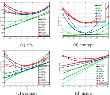
In this section, we would like to evaluate the sum of proposed methods under different cost-sensitive weights. Fig. 2 shows the empirical results under different weights of

an and ap. We find that our proposed algorithms consis-tently outperform all other algorithms under different val-ues of weight on almost all datasets. This further validates the effectiveness of the proposed methods.

4.3 Evaluation with Cost Metrics

4.3.1 Evaluation of Weighted Cost Performance

Table 2 summaries the experimental performance of the ACOGcoston 4 datasets in terms of costmetrics, and Fig. 3 illustrates the development of online cost performance at each iteration.

By evaluating thecostperformance in Fig. 3 and Table 2, our proposed methods achieve much lower misclassifica-tioncostthan other methods among all cases. For example, the overall cost of ACOG is about less than half of cost

made by all regular first-order algorithms (i.e., perceptron, ROMMA, PA-I, PAUM and CPAPB). This implies that intro-ducing the second order information is beneficial to the decrease of misclassificationcost.

In addition, by examining both sensitivety and

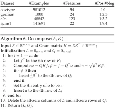
specificitymetrics, we observe that our proposed methods TABLE 1

List of Binary Datasets in Experiments

Dataset #Examples #Features #Pos:#Neg

covtype 581012 54 1:1

german 1000 24 1:2.3

a9a 48842 123 1:3.2

ijcnn1 141691 22 1:9.4

(10)

often achieve the bestsensitivityresult on all datasets, and attain a relatively goodspecificityamong all cases.

Moreover, the diagonal ACOGdiag methods achieve higher cost value than ACOG methods, but their running time are lower. This is similar with the situation based on

summetric. Thus, the ACOGdiag methods can be regarded as a choice to balance the performance and efficiency.

4.3.2 Evaluation of Cost under Varying Weights

In this section, we examine thecostperformance under dif-ferent cost-sensitive weights cn and cp for our proposed algorithms. From the results in Fig. 4, we observe that the proposed algorithms outperform almost all other algo-rithms under different weights. And only on a few datasets, AROW can achieve similar performance with our proposed TABLE 2

Evaluation of the Cost-Sensitive Classification Performance of ACOG and Other Algorithms

Algorithm “sum”on a9a “cost”on a9a

Sum(%) Sensitivity(%) Specificity (%) Time(s) Cost(102₎ _{Sensitivity(%) Specificity (%) Time(s)} Perceptron 71.3430.215 56.4060.327 86.2800.102 0.196 50.9510.382 56.4060.327 86.2800.102 0.191 ROMMA 70.9040.239 57.9180.493 83.8890.262 0.225 50.1840.361 57.9890.346 83.8630.227 0.224 PA-I 71.2740.169 56.3100.277 86.2370.113 0.212 51.0680.311 56.3100.277 86.2370.113 0.212 PAUM 78.2550.155 70.8680.345 85.6430.116 0.192 35.9760.346 70.8680.345 85.6430.116 0.197 CPAPB 72.6780.209 62.8180.345 82.5370.145 0.254 42.5170.326 66.8180.285 79.5030.132 0.246 AROW 75.8540.188 58.8580.510 92.8490.153 5.591 45.9310.486 58.8580.510 92.8490.153 5.104 COG-I 78.9780.128 71.9670.264 85.9900.137 0.192 28.6320.263 79.3900.241 81.2840.107 0.190 COG-II 79.1260.103 81.0380.243 77.2130.168 0.201 25.5270.182 89.0130.171 62.3980.243 0.193 ACOG-I 79.9030.109 73.5610.347 86.2440.162 3.080 26.7600.291 81.1290.340 81.3980.219 2.837 ACOG-II 81.2200.108 85.2690.219 77.1710.134 3.344 20.3070.169 94.0790.136 62.1070.185 3.612 ACOG-Idiag 79.8270.094 73.3610.245 86.2930.103 0.202 26.9170.253 80.9900.282 81.3690.147 0.205 ACOG-IIdiag 81.0980.083 84.7050.227 77.4910.152 0.216 20.6610.110 93.3520.126 63.2120.238 0.213

Algorithm “sum”on covtype “cost”on covtype

Sum(%) Sensitivity(%) Specificity (%) Time(s) Cost(102

) Sensitivity(%) Specificity (%) Time(s) Perceptron 52.6090.057 51.3640.058 53.8540.057 1.649 1377.4641.638 51.3640.058 53.8540.057 1.662 ROMMA 52.1640.674 50.8190.731 53.5090.647 2.233 1391.25019.560 50.8600.702 53.5410.614 2.295 PA-I 51.6660.056 50.3240.061 53.0080.063 1.869 1406.5001.675 50.3240.061 53.0080.063 1.913 PAUM 54.2680.059 52.5880.089 55.9490.066 1.693 1340.0222.311 52.5880.089 55.9490.066 1.709 CPAPB 51.6670.057 50.5520.063 52.7810.065 2.135 1194.4331.911 59.6610.070 44.2750.072 2.199 AROW 63.0360.033 60.1580.244 65.9140.213 22.640 687.6963.148 76.5800.137 69.5790.134 22.556 COG-I 54.2680.059 52.5880.089 55.9490.066 1.637 631.8341.721 84.0360.070 24.4940.062 1.710 COG-II 54.2080.051 54.0380.096 54.3770.055 1.643 426.1220.834 94.0880.031 7.5010.107 1.657 ACOG-I 68.0770.038 70.5650.073 65.5880.082 13.782 466.3761.190 90.6930.049 23.0540.038 18.988 ACOG-II 68.0200.030 71.2650.070 64.7740.068 13.528 305.0560.355 98.9690.021 6.3650.163 13.232 ACOG-Idiag 67.2470.060 69.1830.076 65.3110.082 1.824 469.7011.377 90.5940.090 22.7820.370 1.971 ACOG-IIdiag 67.2250.062 69.9130.096 64.5370.086 1.805 308.9877.944 98.7390.367 7.0150.507 1.828

Algorithm “sum”on german “cost”on german

Sum(%) Sensitivity(%) Specificity (%) Time(s) Cost(102

) Sensitivity(%) Specificity (%) Time(s) Perceptron 53.7601.655 35.1332.343 72.3860.977 0.003 1.9450.070 35.1332.343 72.3860.977 0.003 ROMMA 57.6252.943 43.5504.496 71.7001.710 0.004 1.7210.128 43.6504.372 71.5361.932 0.004 PA-I 53.0431.902 34.0002.818 72.0861.128 0.003 1.9770.083 34.0002.818 72.0861.128 0.003 PAUM 54.1451.335 26.4833.633 81.8071.341 0.003 2.1120.091 26.4833.633 81.8071.341 0.003 CPAPB 53.1851.948 37.8832.925 68.4861.144 0.004 1.7590.082 44.3172.883 63.4641.287 0.004 AROW 59.9481.295 26.3673.893 93.5291.630 0.014 1.6100.082 43.8673.364 86.5711.543 0.016 COG-I 54.4241.474 36.0832.203 72.7640.807 0.003 1.7700.081 42.9333.010 67.2000.990 0.003 COG-II 54.9521.359 54.8331.318 55.0711.442 0.003 1.0350.033 81.0670.799 25.2001.983 0.003 ACOG-I 63.1501.025 49.0501.932 77.2501.489 0.008 1.2320.049 62.7502.017 67.6711.394 0.010 ACOG-II 62.5111.190 63.0002.052 62.0211.408 0.008 0.8750.044 86.8832.264 25.5644.099 0.011 ACOG-Idiag 61.7651.195 47.5172.610 76.0141.022 0.003 1.3300.064 58.9672.362 68.3000.901 0.003 ACOG-IIdiag 62.2811.428 62.8831.852 61.6791.576 0.003 0.9120.045 84.7330.876 28.6294.046 0.003

Algorithm “sum”on ijcnn1 “cost”on ijcnn1

Sum(%) Sensitivity(%) Specificity (%) Time(s) Cost(102₎ _{Sensitivity(%) Specificity (%) Time(s)} Perceptron 69.9880.252 45.9260.455 94.0510.050 0.112 26.3030.221 45.9260.455 94.0510.050 0.114 ROMMA 75.5470.229 57.6890.439 93.4050.111 0.124 21.4670.207 57.6660.459 93.4040.108 0.128 PA-I 69.9800.312 45.5420.579 94.4180.083 0.119 26.3050.274 45.5420.579 94.4180.083 0.124 PAUM 79.0660.275 64.3770.590 93.7550.092 0.112 18.3780.239 64.3770.590 93.7550.092 0.118 CPAPB 73.7450.209 57.3280.371 90.1610.091 0.155 23.0960.200 57.2150.407 90.2330.094 0.160 AROW 67.2580.460 36.2080.980 98.3080.074 0.450 28.6260.401 36.2080.980 98.3080.074 0.465 COG-I 79.0660.275 64.3770.590 93.7550.092 0.109 18.4410.236 64.1710.590 93.8140.096 0.116 COG-II 81.5200.232 81.9400.363 81.1000.182 0.112 16.3980.197 81.6830.311 81.3940.205 0.116 ACOG-I 82.3750.230 71.0100.607 93.7400.178 0.212 15.1970.123 71.9960.352 93.4290.102 0.218 ACOG-II 86.8720.174 88.9240.323 84.8200.218 0.288 12.2790.149 87.6260.293 84.7700.165 0.298 ACOG-Idiag 81.4680.225 69.0070.502 93.9290.092 0.114 15.6810.227 70.6800.624 93.6310.127 0.122 ACOG-IIdiag 86.9290.124 88.2050.266 85.6520.107 0.120 12.0160.111 87.1640.300 85.8010.138 0.122

(11)

methods. These discoveries imply that our ACOG algo-rithms have a wide selection range of weight parameters for online classification tasks.

4.4 Evaluation of Algorithm Properties

We have evaluated the performance of proposed algo-rithms in previous experiments, where promising results confirm their great superiority. Next, we are eager to examine their unique properties, including the influence of learning rate, regularized parameter, updating rule, online estimation and generalization ability. These examinations contribute to better understanding and applications of proposed methods. For simplicity, all experiments are based on sum metric, and every experi-ment only considers one objective or variable, while all other variable settings are fixed and similar with before experiments.

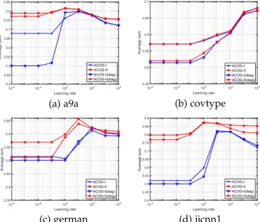
4.4.1 Evaluation of Learning Rate

In this section, we evaluate the influence of learning rate. In detail, we examine the sum performances of propo-sed methods with different learning rates h from ½104_;

103_;_{. . .}_;₁₀3_;₁₀4_.

In Fig. 5, we find that ACOG algorithms would achieve relatively higher result, when we choose proper learning rate (i.e., relatively higher h in general). This is easy to understand because the values of covariance matrix S are normally small. Specifically, when a misclassification happened at timet, we update the predictive vector mby

m_t_þ₁¼m_tþhSt_þ1gt, where gt¼@‘tðmtÞ. Because the values of covariance matrix S are normally small, the values of Stþ1gtthus are small. So if we want to obtain excellent per-formance, it would be better to choose properly higher learning rates as updating steps.

Fig. 1. Evaluation of online “sum“ performance of the proposed algo-rithms on public datasets.

Fig. 2. Evaluation of weighted “sum“ performance under varying weights of sensitivity and specificity.

Fig. 3. Evaluation of online “cost“ performance of the proposed algo-rithms on public datasets.

Fig. 4. Evaluation of weighted “cost“ performance under varying weights for False Positives and False Negatives.

(12)

Moreover, we find the proposed methods with objective function ‘II_ð_w_;_ð_{x; y}_ÞÞ _{can achieve relatively higher} perfor-mance than the methods with ‘I_ð_w_;_ð_{x; y}_ÞÞ_{, which means} that ACOG-II and ACOG-IIdiagare more robust to different learning rate h and consequently have a wider parameter choice space.

4.4.2 Evaluation of Regularized Parameter

Now, we aim to examine the influence of regularized parameters on our proposed algorithms.

When the learner makes a mistake, we update the covari-ance matrixS byStþ1¼StSt

xtx>tSt

gþx>_tStxt with default regular-ized parameter g as 1. However, the rationality of this setting is not verified. Thus, we examine the performance of our algorithms with different regularized parameters g

from½104_;₁₀3_;_{. . .}_;₁₀3_;₁₀4_for_sum_metrics.

The results in Fig. 6 show that the optimal parameter nor-mally is different according to datasets; while in most cases,

the settingg¼1can achieve the best or fairly good results. This discovery confirms the practical value of our algo-rithms with default settings.

4.4.3 Evaluation of Updating Rule

As mentioned in Section 2, the predictive vector m is updated by mtþ1¼mtþhStþ1gt, which is different from AROW where the updating rule formrelies on the oldSt. In this section, we would like to evaluate the difference between two updating rules based onsummetrics for pro-posed methods, where the invariant versions (i.e., green line in Fig. 7) depending on oldSt.

From Fig. 7, we find that although the difference between two updating rules is not obvious, the performance ofStþ1 versions slightly exceed St versions, which is consistent with our analysis in Section 2.

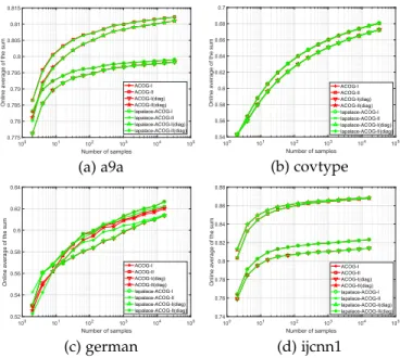
4.4.4 Evaluation of Online Estimation of Tn

Tp

In the remark of Algorithm 1, we analyzed the parameter

r¼h_hpTn

nTp for ACOGsumalgorithms, where the main question is that the value ofTpandTncannot be obtained in advance on real-world online learning.

Thus, we want to evaluate the influence of online estima-tion Tn

Tp on sum performance, compared with the original algorithms. We adopt the widely used laplace estimation here, which estimatesTn

Tp by tnþ1

tpþ1, wheretpand tnrepresent the number of positive samples and negative samples that have been seen, respectively.

Fig. 8 shows the performance of online estimation. We find that the online laplace estimation performs quite similar results with the original one. This discovery validates the practical value of the proposed ACOGsumalgorithms.

4.4.5 Evaluation of Generalization Ability

Then, we evaluate the generalization ability of proposed methods, which may exist problems when converting an online algorithm to a batch training approach. We use

Fig. 5. Performance under varying learning rates.

Fig. 6. Performance under different regularized parameters.

(13)

5-fold cross-validation for better validation of the general performance.

Table 3 summary the consequences on sum metrics, in which we discover that our proposed algorithms achieve the best among all algorithms on all datasets. This discovery indicates that our proposed methods have a strong general-ized ability and can be regarded as a potentially useful tool to train large-scale cost-sensitive models.

4.5 Performance and Efficiency of Sketched ACOG In the previous experiments, the evaluations of the pro-posed ACOG algorithms have shown promising results. However, we can find the implementation of ACOG is time consuming when facing high-dimensional datasets, because of the updating step for covariance matrix. As a result, it is difficult for engineers to address the real-world tasks with quite large-scale datasets.

A simple solution to this question is to implement the diagonal version of ACOG, and then enjoy linear time com-plexity. However, the gain of diagonal ACOG is at the cost of lower performance, because it abandons the correlation information between sample dimensions, which is quite important and indispensable for datasets with strong inner-correlation. Thus, for better trade off between performance and time efficiency, we propose the Sketched ACOG (named SACOG) and its sparse version (named SSACOG).

In this section, we first evaluate our sketched algori-thms with several baseline algorialgori-thms: (1) “COG-I“ and “COG-II“; (2) “ACOG-I“ and “ACOG-II“; (3) “ACOG-Idiag“ and “ACOG-IIdiag“, where we adopt 4 relatively high-dimensional datasets from LIBSVM, which are higher than 45 dimensions as list in Table 4. After that, we examine the performance difference between SACOG and SSACOG.

For simplicity, we focus on the case that the sketch sizem

is fixed as 5 for all sketched algorithms, although our meth-ods can be easily generalized by setting different sketch sizes like [22]. Moreover, the learning rate was selected from ½105_;₁₀4_;_{. . .}_;₁₀5_{, where other implementation details are} similar with [22]. In addition, all experimental settings for other algorithms are same as previous experiments.

4.5.1 Evaluation of Weighted Sum Performance

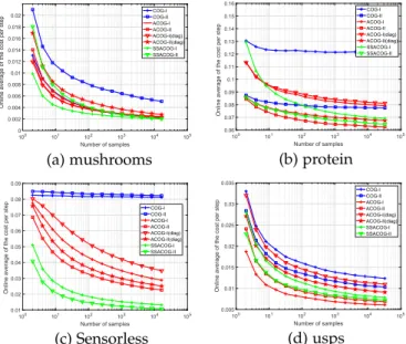
In this section, we would like to examine the performance and efficiency of our sketched algorithms, where we adopt the sparse version (SSACOG) rather than the original SACOG, which is more appropriate for real-world datasets.

The results are summarized in Fig. 9, Fig. 10 and Table 5 based on two metrics, from which we find that the proposed SSACOG is much faster than ACOG algorithms, while the performance of sketched algorithms is not affected too much and sometimes even better. In addition, the degree of efficiency optimization by sketching technique goes up along with the increase of data dimensions, which is consis-tent with the common sense.

Note that although the running time of SSACOG is slower than ACOGdiag, it enjoys higher performance due

Fig. 8. Evaluation of online estimation ofTn Tp.

TABLE 3

Evaluation of Generalization Ability withsum

Algorithm a9a covtype german ijcnn1

Perceptron 68.649 51.553 53.737 70.045 ROMMA 72.467 67.059 58.614 76.818 PA-I 71.986 51.283 51.363 70.410 PAUM 79.323 53.354 52.126 82.012 CPAPB 73.668 51.279 52.768 73.942 AROW 75.961 64.928 54.575 67.642 COG-I 79.705 53.354 52.258 82.012 COG-II 78.559 68.897 50.784 82.849 ACOG-I 80.026 72.428 62.954 82.926 ACOG-II 81.630 72.632 60.928 87.730 ACOG-Idiag 80.118 71.051 64.389 82.334 ACOG-IIdiag 81.752 71.311 66.036 87.628 TABLE 4

Datasets for Evaluation of Sketched Algorithm

mushrooms 8124 112 1:1.07

protein 17766 357 1:1.7

usps 7291 256 1:5.11

Sensorless 58509 48 1:10

(14)

to the advantage of sufficient second-order information. This confirms the superiority of ACOG with sketching technique.

4.5.2 Efficiency Comparison between Sketched ACOG

and Sparse Sketched ACOG

Then, We would like to compare the performance and run-ning time between SACOG and its sparse version SSACOG. The experimental results based on both metrics are summa-rized in Table 6.

From results, we find that the running time of SSACOG is lower than SACOG. It is consistent with the time com-plexity analysis of two algorithms in Section 3. For better understanding, we simply give a analysis. Given sketch size

m¼5, the time complexity for SACOG isOð25dÞaccording to the analysis of Section 3, while the time complexity for SSACOG is Oð125þ5sÞ. One can accelerate the time com-plexity toOð5dÞfor SACOG andOð25þ5sÞfor SSACOG by only updating the sketch everymround.

Thus, the time complexity for SACOG is linear in the data dimensionalityd, and running time for SSACOG is lin-ear in the data non-sparse degrees. Then, it is easy to under-stand the SSACOG would be much faster than SACOG, when the data dimensionalitydis high and the data sparsity is strongsd.

5 A

PPLICATION TO

O

NLINE

A

NOMALY

D

ETECTION The proposed adaptive regularized cost-sensitive online classification algorithms can be potentially applied to solve a wide range of real-world applications in data mining. To verify their practical application value, we apply them to tackle several online anomaly detection tasks in this section. 5.1 Application Domains and Testbeds

Below, we first exhibit the related domains of anomaly detection problems:

Finance: The credit card approval problem enjoys a huge demand in financial domains, where our task is

to discriminate the credit-worthy customers for the Australian dataset from an Australian credit company. Nuclear: We apply our algorithms to the Magic04 dataset with 19020 samples to simulate registration of high gamma particles. The dataset was collected by a ground-based atmospheric Cherenkov gamma telescope. In detail, the “gamma signal“ samples are considered as the normal class, while the hadron ones are treated as outliers.

Bioinformatics: We address bioinformatics anomaly detection problems with DNA dataset to recognize the boundaries between exons and introns from a given DNA sequence, where exon/intron boundaries are defined as anomalies and others are treated as normal. Medical Imaging: We apply our approaches to add-ress the medical image anomaly detection problem with the KDDCUP08 breast cancer dataset4. The main goal is to detect the breast cancer from X-ray images, where “benign” is assigned as normal and “malignant” is abnormal.

To better understand, we summary the detailed informa-tion for each dataset in Table 7.

5.2 Empirical Evaluation Results

In this section, our algorithms are applied to address real-world anomaly detection tasks with 4 datasets from different domains, where we use thebalanced accuracymetric to avoid inflated performance evaluations on imbalanced datasets. In addition, we apply our sparse sketched ACOG algorithms (SSACOG) only for two high-dimensional datasets (i.e., DNA and KDDCUP08), because for low-dimensional tasks, the proposed ACOG algorithms are fast enough. Further-more, all implementation settings are same as Section 4.

Table 8 exhibits the experimental results, from which we can draw several observations. First of all, two cost-sensitive methods (PAUM and CPAPB) outperform their regular methods (Perceptron and PA-I) among all datasets. This confirms the superiority of cost-sensitiveness for online learning. Second, COG algorithms outperform all regular first-order algorithms (i.e., first 5 baselines) on almost all datasets, which demonstrates the effectiveness of direct cost-sensitive optimization in online learning.

Moreover, ACOG algorithms and AROW algorithm out-perform all other algorithms, where ACOG is the updated version of COG with adaptive regularization using second order information. This infers the online classification that introduces the second-order inner-correlation information can enjoy a huge performance improvement. Furthermore, the performance of ACOG exceeds all other algorithms, which demonstrates the effectiveness of cost-sensitive online optimization using the second order information.

By the way, although the speed of SSACOG is slightly slower than ACOGdiag, its performance is relatively better. On the other hand, SSACOG is much faster than ACOG with slight performance loss. This implies that the sketching version of ACOG is a good choice to balance the perfor-mance and efficiency for handling high-dimensional real-world tasks. Furthermore, if someone only wants to pursue the efficiency, they can regard ACOGdiagas a choice.

Fig. 10. Weighted “cost“ performance of SACOG.

(15)

In conclusion, all promising results confirm the superior-ity of our proposed algorithms for real-world online anom-aly detection problems, where datasets are normally high-dimensional and highly class-imbalanced.

6 C

ONCLUSION

In this paper, to remedy the weakness of first-order cost-sensitive online learning algorithms, we propose to TABLE 5

Evaluation of the Cost-Sensitive Classification Performance of SSACOG

Algorithm “sum”on mushrooms “cost”on mushrooms

Sum(%) Sensitivity(%) Specificity (%) Time(s) Cost Sensitivity(%) Specificity (%) Time(s) COG-I 99.2050.047 99.4550.075 98.9560.095 0.019 15.7602.496 99.8230.070 97.6880.091 0.020 COG-II 99.2110.057 99.4200.094 99.0030.097 0.019 39.1802.283 99.5380.055 94.4650.275 0.019 ACOG-I 99.5800.027 99.8100.070 99.3500.076 0.043 18.7351.062 99.9390.051 95.8020.443 0.085 ACOG-II 99.5720.033 99.7940.080 99.3490.075 0.045 16.7701.546 99.9320.035 96.3730.412 0.054 ACOG-Idiag 99.4470.052 99.6520.077 99.2430.087 0.019 17.5201.588 99.9330.045 98.1190.060 0.020 ACOG-IIdiag 99.4570.052 99.6520.086 99.2620.117 0.019 21.1851.431 99.7920.037 96.6010.167 0.019 SSACOG-I 99.6280.052 99.7980.066 99.4590.102 0.038 15.8801.677 99.9300.043 96.6230.303 0.041 SSACOG-II 99.6060.050 99.8050.062 99.4080.093 0.038 15.5603.870 99.8690.040 97.2911.063 0.034

Algorithm “sum”on protein “cost”on protein

Algorithm “sum”on Sensorless “cost”on Sensorless

Algorithm “sum”on usps “cost”on usps

Sum(%) Sensitivity(%) Specificity (%) Time(s) Cost Sensitivity(%) Specificity (%) Time(s) COG-I 96.8200.165 96.3610.345 97.2790.116 0.039 90.1653.851 92.6420.344 98.1790.060 0.031 COG-II 96.5760.139 96.5160.226 96.6370.193 0.038 75.1354.338 96.5700.215 93.7220.342 0.030 ACOG-I 98.0730.115 97.8220.242 98.3230.095 0.271 44.3653.448 96.6710.321 98.5910.070 0.151 ACOG-II 97.6330.148 97.9980.230 97.2680.176 0.239 50.1004.321 98.2410.172 94.8830.488 0.252 ACOG-Idiag 96.8860.226 95.6410.435 98.1310.076 0.039 79.8504.773 93.5260.423 98.3140.080 0.031 ACOG-IIdiag 96.3050.182 96.3690.228 96.2400.182 0.040 66.3003.242 96.9930.149 94.4250.295 0.030 SSACOG-I 97.0910.197 96.8170.323 97.3650.125 0.077 57.0554.251 95.6570.384 98.2960.076 0.054 SSACOG-II 97.0480.163 97.0100.237 97.0850.190 0.074 52.4204.009 97.6470.192 95.5500.360 0.054 TABLE 6

Evaluation between SACOG and Sparse SACOG

Algorithm “sum”on mushrooms “cost”on mushrooms “sum”on protein “cost”on protein

Sum(%) Time(s) Cost(102

) Time(s) Sum(%) Time(s) Cost(102

) Time(s)

SACOG-I 99.6200.043 0.072 16.0201.796 0.096 71.5440.197 3.769 1226.89017.094 3.302

SACOG-II 99.5980.040 0.074 13.7901.852 0.035 71.9070.180 3.705 1147.77514.364 2.373

SSACOG-I 99.6280.052 0.038 15.8801.677 0.039 71.5320.198 0.287 1227.34516.904 0.272

SSACOG-II 99.6060.050 0.038 15.5603.870 0.033 71.9000.204 0.285 1144.68013.087 0.239

Algorithm “sum”on Sensorless “cost”on Sensorless “sum”on usps “cost”on usps

Sum(%) Time(s) Cost(102

) Time(s) Sum(%) Time(s) Cost(102

) Time(s)

SACOG-I 92.4320.213 0.232 753.69521.185 0.235 97.1460.149 0.135 55.9703.053 0.078

SACOG-II 93.9130.129 0.193 615.62512.280 0.194 97.0710.169 0.091 53.1554.815 0.090

SSACOG-I 92.4320.213 0.239 753.69521.185 0.225 97.0910.197 0.057 57.0554.251 0.052

(16)

introduce second-order information into cost-sensitive online classification framework based on adaptive regulari-zation. As a result, a family of second-order cost-sensitive online classification algorithms is proposed, with favour-able regret bound and impressive properties.

Moreover, to overcome the time-consuming problem of our second-order algorithms, we further study the sketch-ing method in cost-sensitive online classification frame-work, and then propose sketched cost-sensitive online classification algorithms, which can be developed as a sparse cost-sensitive online learning approach, with better trade off between the performance and efficiency.

Then for examination of the performance and efficiency, we empirically evaluate our proposed algorithms on many public real-world datasets in extensive experiments. Promis-ing results not only prove the new proposed algorithms suc-cessfully overcome the limitation of first-order algorithms, but also confirm their effectiveness and efficiency in solving real-world cost-sensitive online classification problems.

Future works include: (i) further exploration about the in-depth theory of cost-sensitive online learning; (ii) further study about the sparse computation methods in cost-sensitive online classification problems.

A

CKNOWLEDGMENTS

This research is partly supported by the National Research Foundation, Prime Ministers Office, Singapore under its International Research Centres in Singapore Funding Initia-tive, and partly supported by the National Natural Science Foundation of China (NSFC) under Grant 61602185, and the Fundamental Research Funds for the Central Universities under Grant D2172480. Y. Zhang is the co-first author with equal contribution.

R

EFERENCES

[1] F. Rosenblatt, “The perceptron: A probabilistic model for informa-tion storage and organizainforma-tion in the brain,” Psychological Rev., vol. 65, no. 6, 1958, Art. no. 386.

[2] P. Zhao, S. C. Hoi, and R. Jin, “Double updating online learning,” J. Mach. Learn. Res., vol. 12, pp. 1587–1615, 2011.

[3] J. Wang, P. Zhao, and S. C. Hoi, “Exact soft confidence-weighted learning,” inProc. Int. Conf. Mach. Learn., 2012, pp. 107–114. [4] Q. Wu, H. Wu, X. Zhou, M. Tan, Y. Xu, Y. Yan, and T. Hao,

“Online transfer learning with multiple homogeneous or hetero-geneous sources,”IEEE Trans. Knowl. Data Eng., vol. 29, no. 7, pp. 1494–1507, Jul. 2017.

[5] P. Zhao and S. C. Hoi, “Cost-sensitive online active learning with application to malicious URL detection,” inProc. ACM Int. Conf. Knowl. Discovery Data Mining, 2013, pp. 919–927.

[6] S. C. Hoi, D. Sahoo, J. Lu, and P. Zhao, “Online learning: A com-prehensive survey, ” arXiv preprint arXiv:1802.02871, 2018. [7] J. Ma, L. K. Saul, S. Savage, and G. M. Voelker, “Learning to detect

malicious urls,”ACM Trans. Intell. Syst. Technol., vol. 2, no. 3, 2011, Art. no. 30.

[8] B. Li, S. C. Hoi, P. Zhao, and V. Gopalkrishnan, “Confidence weighted mean reversion strategy for online portfolio selec-tion,” ACM Trans. Knowl. Discovery Data, vol. 7, no. 1, 2013, Art. no. 4.

[9] S. Shalev-Shwartz, Y. Singer, N. Srebro, and A. Cotter, “Pegasos: Primal estimated sub-gradient solver for SVM,”Math. Program., vol. 127, no. 1, pp. 3–30, 2011.

[10] C. Elkan, “The foundations of cost-sensitive learning,” inProc. Int. Joint Conf. Artif. Intell., pp. 973–978, vol. 17, 2001.

[11] K. Veropoulos, C. Campbell, and N. Cristianini, “Controlling the sensitivity of support vector machines,” in Proc. Int. Joint Conf. Artif. Intell., 1999, pp. 55–60.

[12] H. He and E. A. Garcia, “Learning from imbalanced data,” IEEE Trans. Knowl. Data Eng., vol. 21, no. 9, pp. 1263–1284, Sep. 2009.

[13] J. Han, J. Pei, and M. Kamber, “Data mining: Concepts and techniques,” Elsevier, 2011.

[14] K. H. Brodersen, C. S. Ong, K. E. Stephan, and J. M. Buhmann, “The balanced accuracy and its posterior distribution,” inProc. Int. Conf. Pattern Recognit., 2010, pp. 3121–3124.

[15] R. Akbani, S. Kwek, and N. Japkowicz, “Applying support vector machines to imbalanced datasets,” inProc. Eur. Conf. Mach. Learn., 2004, pp. 39–50.

[16] J. Wang, P. Zhao, and S. C. H. Hoi, “Cost-sensitive online classi-fication,” inProc. IEEE Int. Conf. Data Mining, 2012, 1140–1145. [17] J. Wang, P. Zhao, and S. C. H. Hoi, “Cost-sensitive online

classi-fication,”IEEE Trans. Knowl. Data Eng., vol. 26, no. 10, pp. 2425– 2438, Oct. 2014.

[18] M. Dredze, K. Crammer, and F. Pereira, “Confidence-weighted linear classification,” inProc. Int. Conf. Mach. Learn., 2008, 264–271. [19] K. Crammer, M. Dredze, and F. Pereira, “Exact convex confi-dence-weighted learning,” in Proc. Advances Neural Inf. Process. Syst., 2009, pp. 345–352.

[20] K. Crammer, A. Kulesza, and M. Dredze, “Adaptive regulariza-tion of weight vectors,” inProc. Advances Neural Inf. Process. Syst., 2009, pp. 414–422.

TABLE 7

Datasets for Online Anomaly Detection

Australian 690 14 1:1.25

Magic04 19020 10 1:1.8

DNA 2000 180 1:3.31

KDDCUP08 102294 117 1:163.19

TABLE 8

Evaluation for Online Anomaly Detection Algorithm “sum”on Australian “sum”on Magic04

Sum(%) Time(s) Sum(%) Time(s)

Perceptron 57.8631.327 0.002 59.1540.408 0.030 ROMMA 58.7323.462 0.002 64.0253.277 0.042 PA-I 57.1031.595 0.002 58.0290.312 0.036 PAUM 62.3620.941 0.002 64.6710.204 0.030 CPAPB 57.1101.599 0.003 58.4480.360 0.043 AROW 67.1740.749 0.008 70.8960.190 0.154 COG-I 65.9720.879 0.002 65.9130.189 0.030 COG-II 67.2130.787 0.002 69.8150.183 0.030 ACOG-I 68.8080.894 0.005 72.9350.186 0.088 ACOG-II 69.2280.733 0.005 68.3451.822 0.092 ACOG-Idiag 68.4640.936 0.002 73.2680.158 0.033 ACOG-IIdiag 68.5100.917 0.002 73.0350.187 0.033

Algorithm “sum”on DNA “sum”on KDDCUP08

Sum(%) Time(s) Sum(%) Time(s)

Perceptron 84.7590.575 0.006 54.0181.056 0.376 ROMMA 85.7820.553 0.006 54.3421.581 0.507 PA-I 87.8320.833 0.005 54.0530.865 0.414 PAUM 88.5600.737 0.005 55.1610.424 0.386 CPAPB 89.4010.645 0.007 57.3180.629 0.458 AROW 89.1830.405 0.269 50.6110.422 12.554 COG-I 87.8860.812 0.006 54.0941.047 0.355 COG-II 87.3950.530 0.005 69.3120.475 0.359 ACOG-I 91.4900.416 0.104 55.0880.936 4.531 ACOG-II 90.8720.677 0.234 71.9202.016 5.803 ACOG-Idiag 89.4980.633 0.006 55.2930.852 0.384 ACOG-IIdiag 88.4330.490 0.006 71.6611.334 0.397 SSACOG-I 89.9750.516 0.016 55.7110.812 0.810 SSACOG-II 90.4440.471 0.023 70.9471.179 0.842