Learning Backtrackless Aligned-Spatial Graph
Convolutional Networks for Graph Classification
Lu Bai, Lixin Cui
∗, Yuhang Jiao, Luca Rossi, Edwin R. Hancock,
IEEE Fellow
Abstract—In this paper, we develop a novel Backtrackless Aligned-Spatial Graph Convolutional Network (BASGCN) model to learn effective features for graph classification. Our idea is to transform arbitrary-sized graphs into fixed-sized backtrackless aligned grid structures and define a new spatial graph convolu-tion operaconvolu-tion associated with the grid structures. We show that the proposed BASGCN model not only reduces the problems of information loss and imprecise information representation arising in existing spatially-based Graph Convolutional Network (GCN) models, but also bridges the theoretical gap between traditional Convolutional Neural Network (CNN) models and spatially-based GCN models. Furthermore, the proposed BASGCN model can both adaptively discriminate the importance between specified vertices during the convolution process and reduce the notorious tottering problem of existing spatially-based GCNs related to the Weisfeiler-Lehman algorithm, explaining the effectiveness of the proposed model. Experiments on standard graph datasets demonstrate the effectiveness of the proposed model.
Index Terms—Graph Convolutional Networks, Transitive Ver-tex Alignment, Backtrackless Walk.
I. INTRODUCTION
G
Raph based representations are powerful tools to mod-el complex systems that involve data lying on non-Euclidean spaces and that are naturally described in terms of relations between their components [1], ranging from chemical compounds [2] to point clouds [3] and social networks [4]. One fundamental challenge arising in the analysis of graph-based data is how to convert graph structures into numeric representations where standard machine learning techniques can be directly employed for graph classification or clustering. The aim of this paper is to develop a new Graph Convolu-tional Network (GCN) model to learn effective features for graph classification. Our idea is to transform arbitrary-sized graphs into fixed-sized backtrackless aligned grid structures and define a new backtrackless spatial graph convolution operation associated with the grid structures. We show that the proposed model not only bridges the theoretical gap between traditional Convolutional Neural Network (CNN) models and spatially-based GCN models, but also significantly reduces the notorious tottering problem of existing spatially-based GCNs related to the Weisfeiler-Lehman algorithm.A. Literature Review
Broadly speaking, in the last three decades most classical state-of-the-art methods for the analysis of graph structures can
Lu Bai ([email protected]), Lixin Cui (∗Corresponding Author:
[email protected]), and Yuhang Jiao are with Central University of Finance and Economics, Beijing, China. Luca Rossi is with Queen Mary University of London, UK. Edwin R. Hancock is with University of York, York, UK.
be separated into two categories, namely a) graph embedding methods and b) graph kernels. Approaches falling in the first category aim to convert graphs into elements of a vectorial space [5], [6], [7], [8], [9] where standard machine learning algorithms can be directly employed for graph data analysis. Unfortunately, these embedding methods tend to approximate structural correlations of graphs in a low dimensional pattern space, leading to structural information loss. To overcome this shortcoming, the proponents of graph kernel approaches suggest to characterize graph structures in a high dimensional Hilbert space and thus better preserve the structural informa-tion [10], [11], [2], [12], [13], [14]. One common limitainforma-tion shared by both graph embedding methods and kernels is that of ignoring information from multiple graphs. This is because graph embedding methods usually capture structural features of individual graphs, while graph kernels reflect structural characteristics for pairs of graphs. Furthermore, since the process of computing the structural characteristics are separate from the classifier, both the graph embedding and kernel methods cannot provide an end-to-end learning architecture that simultaneously integrates the processes of graph charac-teristics learning and graph classification. In summary, these drawbacks influence the effectiveness of employing these traditional methods on graph classification tasks.
In recent years, due to the tremendous successes of deep learning networks in machine learning, there has been an increasing interest to generalize deep Convolutional Neural Networks (CNN) [15], [16], [17], [18], [19] to the graph domain. These novel deep learning networks on graphs are the so-called Graph Convolutional Networks (GCN) [20] and have proven to be an effective way to extract highly mean-ingful statistical features for graph classification [21]. Gener-ally speaking, most existing state-of-the-art GCN approaches can be divided into two main categories, i.e., GCN models based on a) spectral and b) spatial strategies. Specifically, approaches based on the spectral strategy define a convolution operation based on spectral graph theory [22], [23], [24]. By transforming the graph into the spectral domain through the eigenvectors of the Laplacian matrix, these methods perform the filter operation by multiplying the graph by a series of filter coefficients. For instance, Bruna et al. [22] have developed a graph convolution network by defining a spectral filter based on computing the eigen-decomposition of the graph Laplacian matrix. To overcome the expensive computational complexity of the eigen-decomposition, Defferrard et al. [21] have approximated the spectral filters based on the Chebyshev expansion of the graph Laplacian. Unfortunately, most of the spectral-based approaches cannot be performed on graphs
with different number of vertices and Fourier bases. Thus, these approaches work on same-sized graph structures and are usually employed for vertex classification tasks.
On the other hand, approaches based on the spatial strat-egy are not restricted to same-sized graph structures. These approaches generalize the graph convolution operation to the spatial structure of a graph by directly defining an operation on neighboring vertices [25], [26], [27], [28], [29], [30]. For example, Duvenaud et al. [26] have proposed a spatially-based GCN model by defining a spatial graph convolution operation on the 1-layer neighboring vertices to simulate the traditional circular fingerprint. Atwood and Towsley [25] have proposed a spatially-based GCN model by performing spatial graph convolution operations on different layers of neigh-boring vertices rooted at a vertex. Although these spatially-based GCN models can be directly applied to real-world graph classification problems, they still need to further transform the multi-scale features learned from graph convolution layers into fixed-sized representations, so that the standard classifiers can be directly adopted for classifications. One way to achieve this is to directly sum up the learned local-level vertex features from the graph convolution operation as global-level graph features through a SumPooling layer. Since it is difficult to learn rich local vertex topological information from the global features, these spatially-based GCN methods associated with SumPooling have relatively poor performance on graph classification.
To overcome the above shortcoming of existing spatially-based GCN models, Zhang et al. [31] have developed a novel spatially-based Deep Graph Convolutional Neural Network (DGCNN) model to preserve more vertex information. Specif-ically, they propose a new SortPooling layer to transform the extracted vertex features of unordered vertices from the spatial graph convolution layers into a fixed-sized local-level vertex grid structure. This is done by sequentially preserving a specified number of vertices with prior orders. With the fixed-sized grid structures of graphs to hand, a traditional CNN model followed by a Softmax layer can be directly employed for graph classification. Nieper et al. [32], on the other hand, have developed a different spatially-based Patchy-San Graph Convolutional Neural Network (PSGCNN) model to capture more vertex information through local neighbor vertices. Specifically, they extract and normalize a fixed-sized local neighborhood rooted at each vertex, where the vertices of each neighborhood are re-ordered based on the same graph labeling method and graph canonization tool. Since the normalized neighborhood can serve as the receptive field of its root vertex for the convolutional operation, this procedure naturally forms a local-level fixed-sized vertex grid structure for each graph. Thus, the graph convolution operation can be performed by sliding a fixed-sized classical standard convolutional filter over the neighboring vertices, i.e., the convolutional operation is similar to that performed on images with standard convolutional neural networks.
Although both the spatially-based DGCNN and PSGCNN models can capture rich graph characteristics residing on local-level vertices and outperform state-of-the-art GCN models on graph classification tasks, these methods establish the vertex
order based on each individual graph. Thus, they cannot accurately reflect the topological correspondence information between graph structures. Moreover, both models lead to sig-nificant information loss, since those vertices associated with a lower ranking may be discarded. Finally, it has been shown in [31] that most existing spatially-based GCN models [25], [26], [27] are related to the classical Weisfeiler-Lehman (WL) algorithm [11], [14]. This is because the required convolution operation of these GCN models relies on aggregating the features of each vertex as well as its neighboring vertices, in a process that is similar to the WL algorithm, which propagates the features between each vertex and its neighboring vertices. Thus, similarly to the classical WL algorithm, these GCN models may also suffer from the well-known tottering prob-lem [13]. In other words, these GCN models may propagate the feature information from the starting vertex to a second vertex and then immediately propagate the information back to the starting vertex, resulting in the creation of redundant feature information.
B. Contributions
The aim of this paper is to address the shortcomings of existing methods by developing a novel Backtrackless Aligned-Spatial Graph Convolutional Network (BASGCN) model for graph classification tasks. To this end, we develop our recent work in [33] one step further and generalize the original Aligned-Spatial GCN (ASGCN) model [33] to a new backtrackless GCN model which reduces the aforementioned tottering problem. One key innovation of the new model is that of transitively aligning vertices between graphs. That is, given three vertices v, w and xfrom three different sample graphs, if v andx are aligned, andw andxare aligned, the proposed model can guarantee that v andware also aligned. More specifically, similarly to the original ASGCN model, the proposed BASGCN model employs the transitive alignment procedure to transform arbitrary-sized graphs into fixed-sized aligned grid structures with consistent vertex orders, guaran-teeing that the vertices on the same spatial position are also transitively aligned to each other in terms of the topological structures.
Since the process of constructing the grid structure does not discard any vertex, the proposed BASGCN model preserves the advantage of the original ASGCN model, i.e., it reduces the problems of information loss and imprecise information representation arising in existing spatially-based GCNs as-sociated with SortPooling or SumPooling layers [21], [31]. Furthermore, the aligned grid structure of the proposed BAS-GCN model is a kind of backtrackless grid structure, i.e., it corresponds to a directed graph rather than an undirected graph as in the original ASGCN model. Since the spatial graph con-volution operation propagates the vertex feature information along the edges, the nature of the backtrackless grid implies that the information cannot be immediately propagated back to the starting vertex. Thus, this backtrackless structure provides a natural way to define a novel backtrackless spatial graph convolution operation that restricts the well-known tottering problem of existing spatially-based GCNs related to the WL
G𝑝(𝑉𝑝, 𝐸𝑝) ∈ 𝐆
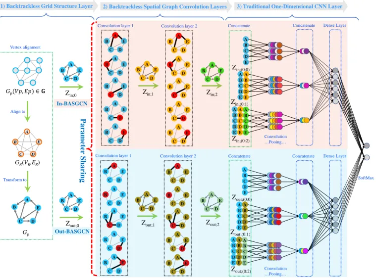
1) Backtrackless Grid Structure Layer
A B E C D G𝑅(VR,ER) Align to Zin;0 A B C D E A B C D E A B C D E A B C D E A B C D E A B C D E A B E C D A B E C D A B E C D A B E C D A B E C D Convolution layer 1 A B E C D A B E C D A B E C D A B E C D A B E C D A B E C D Convolution layer 2 Vertex alignment Concatenate
2) Backtrackless Spatial Graph Convolution Layers 3) Traditional One-Dimensional CNN Layer
Dense Layer A B C D E A B C D E A B C D E A B C D E A B C D E A B C D E Concatenate Convolution …Pooing… A B E C D A B E C D A B E C D A B E C D A B E C D Convolution layer 1 A B E C D A B E C D A B E C D A B E C D A B E C D
Convolution layer 2 Concatenate
A B E C D Transform to G𝑝 A B E C D A B E C D A B E C D A B E C D A B E C D SoftMax In-BASGCN Out-BASGCN Convolution …Pooing… Parameter Sh arin g
Concatenate Dense Layer
Zout;0 Zin;1 Zin;2 Zin;(0:0) Zin;(0:1) Zin;(0:2) Zout;1 Zout;2 Zout;(0:0) Zout;(0:1) Zout;(0:2)
Fig. 1. The architecture of the proposed BASGCN model (vertex features are visualized as different colors). An input graphGp(Vp, Ep)∈Gof arbitrary size is first aligned to the prototype graphGR(VR, ER). Then,Gpis mapped into a fixed-sized backtrackless aligned vertex grid structure, where the vertex order follows that ofGRand the associated aligned vertex adjacency matrix corresponds to a directed graph, i.e., the connection between a pair of vertices is a directed edge. The grid structure ofGpis passed through a pair of parallel stacked spatial graph convolution layers to extract multi-scale vertex features (i.e.,Zin;0andZout;0are the same), where the vertex information is propagated between specified vertices associated with the directed adjacency matrix.
More formally, for each rooted vertex the upper convolution layers focus on aggregating the vertex features of the vertex itself as well as its in-neighbors (i.e., the vertices having directed edges to the rooted vertex), while the lower convolution layers focus on aggregating vertex features of the vertex itself as well as its out-neighbors (i.e., the vertices having directed edges from the rooted vertex to themselves). Note that both the upper and lower graph convolution layers share the same trainable parameters.In the process of vertex information aggregation, the information is propagated along the directed edges, thus the information will not be immediately propagated back to the starting vertex, restricting the tottering problem. Moreover, since the graph convolution layers preserve the original vertex order of the input grid structure, the concatenated vertex features through the graph convolution layers form a new vertex grid structure forGp. This vertex grid structure is then passed to a traditional CNN layer for classification.
algorithm [11]. As a result, the new proposed BASGCN model not only inherits all the advantages of the original ASGCN model, but alsofurther generalizes the original model to a new backtrackless GCN model that reduces the tottering problem and thus reflects richer graph characteristics (see details in Sec.IV-C). The conceptual framework of the proposed BASGCN model is shown in Fig.1. Specifically, the main contributions of this work are threefold.
First, we introduce a new transitive vertex alignment method to map different arbitrary-sized graphs into fixed-sized backtrackless aligned grid structures, i.e., the aligned vertex grid structure as well as the associated backtrackless aligned vertex adjacency matrix. We show that the grid structures not only establish reliable vertex correspondence information between graphs, but also minimize the loss of structural information from the original graphs. Moreover, since the
associated grid structure corresponds to a directed graph, it provides a natural backtrackless structure to restrict the tottering problem.
Second, we develop a novel backtrackless spatially-based graph convolution model, i.e., the BASGCN model, for graph classification. More specifically, we propose a new backtrack-less spatial graph convolution operation to extract multi-scale local-level vertex features. Unlike most existing spatially-based GCN models [25], [26], [27], [31] as well as the AS-GCN model [33], which propagate features between vertices through the original vertex adjacency matrix or the undirected aligned vertex adjacency matrix, the proposed graph convolu-tion layer propagates the feature informaconvolu-tion between aligned grid vertices through the associated backtrackless adjacency matrix. Since the backtrackless adjacency matrix corresponds to a directed graph and provides a natural backtrackless
structure, the proposed graph convolution operation can signif-icantly restrict the tottering problem of most existing spatially-based GCNs as well as the original ASGCN model. More-over, we show that the proposed convolution operation not only reduces the problems of information loss and imprecise information representation arising in existing spatially-based GCN models associated with SortPooling or SumPooling, but also theoretically relates to the classical convolution operation on standard grid structures. Thus, the proposed BASGCN model bridges the theoretical gap between traditional CNN models and spatially-based GCN models, and can adaptively discriminate the importance between specified vertices during the process of spatial graph convolution operations. Finally, since our backtrackless spatial graph convolution operation does not change the original spatial sequence of vertices, the proposed BASGCN model utilizes the traditional CNN to further learn graph features. In this way, we provide an end-to-end deep learning architecture that integrates the graph representation learning into both the backtrackless spatial graph convolutional layer and the traditional convolution layer for graph classification.
Third, we empirically evaluate the performance of the proposed BASGCN model on graph classification tasks. Ex-periments on widely used benchmarks demonstrate the effec-tiveness of the proposed method, when compared to state-of-the-art methods.
The remainder of this paper is organized as follows. Sec-tion II briefly reviews the existing spatially-based GCN mod-els. Section III introduces how to transform different arbitrary-sized graphs into fixed-arbitrary-sized backtrackless aligned grid struc-tures. Section IV details the concept of the proposed BASGCN model. Section V provides the experimental evaluation of the new method. Section VI concludes this work.
II. RELATEDWORKS OFSPATIALLY-BASEDGCN MODELS
In this section, we briefly review state-of-the art spatially-based GCN models in the literature. More specifically, we introduce the associated spatial graph convolution operation of the existing spatially-based Deep Graph Convolutional Neural Network (DGCNN) model [31]. We refer this DGCNN model as a representative approach to analyze the common drawbacks arising in most existing spatially-based GCN models. To commence, consider a sample graph Gwithnvertices, X= (x1, x2, ..., xn)∈ Rn×c is the collection of n vertex feature
vectors of G in c dimensions, and A ∈ Rn×n is the vertex
adjacency matrix (A can be a weighted adjacency matrix). The spatial graph convolution operation of the DGCNN model takes the following form
Z= f( ˜D−1AXW˜ ), (1)
where A˜ = A + I is the adjacency matrix of graph G with added self-loops, D˜ is the degree matrix of A˜ with
˜
A[i,i]=PjA˜[i,j],W ∈Rc×c
0
is the matrix of trainable graph convolution parameters, f is a nonlinear activation function, andZ ∈Rn×c
0
is the output of the convolution operation. For the spatial graph convolution operation defined by Eq.(1), the processXW first maps the c-dimensional features
of each vertex into a set of newc0-dimensional features. Here, the filter weightsW are shared by all vertices. Moreover,AY˜ (Y :=XW) aggregates the feature information of each vertex to its neighboring vertices as well as the vertex itself. The i-th row ( ˜AY)[i,:] represents the extracted features of the i-th vertex, and corresponds to the summation or aggregation of Y[i,:] itself and Y[j,:] from its neighbor vertices. Multiplying by the inverse of D˜ (i.e., D˜−1) can be seen as the process of normalizing and assigning equal weights between the i-th vertex and each of its neighbours.
Although the DGCNN model associated with convolution operation defined by Eq.(1) has been proven a powerful GCN model for graph classification, it still suffers from the following two common drawbacks that arise in most existing spatially-based GCN models [25], [26], [27], [31].
Remark (Less Discrimination between Vertices): Eq.(1) indicates that the spatial graph convolution operation of the DGCNN model cannot discriminate the importance between specified vertices in the convolution operation process. This is because the required filter weights W are shared by each vertex, i.e., the feature transformations of the vertices are all based on the same trainable function. Thus, the DGCNN model cannot directly influence the aggregation process of the vertex features. In fact, this problem also arises in other spatially-based GCN models that utilize the adjacency matrix for vertex information propagation, e.g., the Neural Graph Fingerprint Network (NGFN) model [26], the Diffusion Convolution Neural Network (DCNN) model [25], etc. Since the associated spatial graph convolution operations of these models also take the similar form with that of the DGCNN model, i.e., the trainable parameters of their spatial graph convolution operations are also shared by each vertex. This drawback influences the effectiveness of the existing spatially-based GCN models for graph classification. 2 Remark (Tottering Problems between Vertices): Zhang et al. [31] have indicated the theoretical relationship between the DGCNN model and the classical WL algorithm [11]. The key idea of the WL method is to concatenate a vertex label with the labels of its neighboring vertices, and then sort the concatenated label lexicographically to assign each vertex a new label. The procedure repeats until a maximum iteration h, and each vertex label at an iteration h corresponds to a subtree of height h rooted at the vertex. If the concatenated label of two vertices are the same, the subtree rooted at the two vertices are isomorphic. To exhibit the relationship between the associated graph convolution operation of the DGCNN model defined by Eq.(1) and the WL algorithm, we decompose Eq.(1) into a row-wise manner, i.e.,
Z[i,:]= Relu([ ˜D−1A˜][i,:]Y) = Relu[ ˜D −1 [i,i](Y[i,:]+ X j∈Γ(i) Y[j,:])], (2) whereY := XW and Γ(i) corresponds to the set of neigh-boring vertices of the i-th vertices. For Eq.(2), Y[i,:] can be seen as the continuous valued vectorial vertex label of the i-th vertex. In a manner similar to i-the WL mei-thod, for each
i-th vertex and its associated continuous label Y[i,:] Eq.(2) needs to propagate the continuous labels Y[j,:] of its neigh-boring vertices to its original label Y[j,:] as its new signature vector D˜−[i,i1](Y[i,:]+Pj∈Γ(i)Y[j,:]). The Relu function maps
˜
D−[i,i1](Y[i,:] +Pj∈Γ(i)Y[j,:]) to a new continuous vectorial label. As a result, the graph convolution operation defined by Eq.(2) can be seen as a soft version of the original WL algorithm, explaining the effectiveness of the DGCNN model. Unfortunately, similar to the classical WL algorithm, the DGC-NN model also suffers from the tottering problem arising in the WL algorithm [13]. This is because, like the WL algorithm, the DGCNN model may propagate the feature information from the starting vertex to a vertex at the current convolution layer and then immediately propagate the information back to the starting vertex at the next convolution layer, resulting in redundant feature information. In fact, this problem also arises in other spatially-based GCN models [25], [26], influencing
their performance. 2
III. CONSTRUCTINGALIGNEDBACKTRACKLESSGRID
STRUCTURES FORARBITRARYGRAPHS
Although, spatially-based GCN models are not restricted to the same graph structure, and can thus be applied for graph classification tasks. These methods still need to further transform the extracted multi-scale features from graph con-volution layers into the fixed-sized characteristics through a SumPooling or SortPooling, so that the standard classifiers (e.g., the traditional convolutional neural network followed by a Softmax layer) can be directly employed for classifica-tions. Unfortunately, these pooling operations usually cause information loss. In this section, we develop a transitive matching method to map different graphs of arbitrary sizes into fixed-sized backtrackless aligned grid structures, that can be directly utilized by the spatial graph convolution operation. Moreover, we show that the proposed grid structure not only integrates precise structural correspondence information but also minimizes the loss of structural information. Finally, we show that the proposed grid structure can provide a natural backtrackless structure to reduce the tottering problem arising in existing spatially-based GCN models.
A. Identifying Transitive Vertex Alignment Information
We introduce a new graph matching method to transitively align graph vertices. We first designate a family of prototype representations that encapsulate the principle characteristics over all vectorial vertex representations in a set of graphs G. Assume there are n vertices from all graphs in G, and their associated K-dimensional vectorial representations are RK ={RK
1 ,RK2 , . . . ,RKn}. We utilizek-means [34] to locate M centroids overRK, by minimizing the objective function
arg min Ω M X j=1 X RK i ∈cj kRKi −µKj k2, (3)
where Ω = (c1, c2, . . . , cM) represents M clusters, and µKj the mean of the vertex representations belonging to the j-th cluster cj.
Assume G={G1,· · ·, Gp,· · · , GN} is the graph sample set, where Gp(Vp, Ep) ∈ G is a sample graph of G. For Gp(Vp, Ep) and each vertex vi ∈ Vp associated with its K-dimensional vectorial representation RK
p;i, we initiate by locating a family ofK-dimensional prototype representations as PRK = {µK
1, . . . , µKj , . . . , µKM} for the graphs over G. To establish transitive correspondence information between different graphs, we follow the alignment procedure introduced by Bai et al. [13] for point matching in a pattern space. More formally, we align the vectorial vertex representations of each graph Gp to the family of prototype representations inPRK, by computing a K-level affinity matrix in terms of the Euclidean distances between the two sets of points, i.e.,
AKp(i, j) =kRKp;i−µKj k2. (4) whereAK
p is a |Vp| ×M matrix, and each elementAKp(i, j) corresponds to the value of the distance between RK
p;i and µK
j ∈ PR
K
. If the element AK
p (i, j) is the smallest one in rowi, we say that the vectorial representationRK
p;iofv∈Vpis aligned to thej-th prototype representation µK
j ∈PR
K, i.e., the vertex vi is aligned to the j-th prototype representation. Note that for each graph there may be multiple vertices aligned to the same prototype representation. We record the correspondence information using theK-level correspondence matrixCpK ∈ {0,1}|Vp|×M
CpK(i, j) =
1 ifAKp (i, j) is the smallest in rowi
0 otherwise.
(5) For each pair of graphs Gp ∈ G and Gq ∈ G, if their vertices vp and vq are aligned to the same prototype representation µKj ∈ PRK, we say that vp and vq are also aligned. Thus, we identify the transitive correspondence information between all graphs in G, by aligning their vertices to a common set of prototype representations.
Remark: The alignment process is equivalent to assigning the vectorial representation RKp;i of each vertex vi ∈ Vp to the meanµK
j of the clustercj. Thus, the proposed alignment procedure can be seen as an optimization process that grad-ually minimizes the inner-vertex-cluster sum of squares over the vertices of all graphs through k-means, and can establish reliable vertex correspondence information over all graphs.2
B. Aligned Grid Structures of Graphs
We employ the transitive correspondence information to map arbitrary-sized graphs into fixed-sized backtrackless aligned grid structures,i.e., the aligned vertex grid structures as well as the associated backtrackless aligned vertex adjacency matrices. Assume Gp(Vp, Ep,Ap˜ ) is a sample graph from the graph set G, withVp representing the vertex set, Ep representing the edge set, and Ap¯ representing the vertex adjacency matrix with added self-loops (i.e.,A˜=A+I, where A is the original adjacency matrix with no self-loops andIis the identity matrix). LetXp ∈Rn×c be the collection
ofn(n=|Vp|) vertex feature vectors ofGp inc dimensions. Note that, the row of Xp follows the same vertex order of
G1 G𝑝 G𝑁
…
…
…
…
G𝑝 v1 𝐃𝐁𝒑;𝟐𝑲 [𝐻𝑆(𝐺𝑝;21 ),𝐻𝑆(𝐺𝑝;22 ),…, 𝐻𝑆(𝐺𝑝;2𝐾 )]T 1…
…
Compute K-dimensional DB representations Compute M K-dimensional prototype representations μ1𝐾 μ𝑗𝐾 μ𝑀𝐾…
…
Compute K-level correspondence matrix𝑃𝑅
1𝐿 𝑪𝒑𝑲(𝒊, 𝒋) ∈ (𝟎, 𝟏) 𝑃𝑅1𝐾 𝑃𝑅𝑗𝐾 𝑃𝑅𝑀𝐾 DB𝑝;|𝑉|𝐾 DB𝑝;1𝐾 DB𝑝;𝑖𝐾 𝒗𝒆𝒓𝒕𝒆𝒙 𝟐…
…
G𝑅…
2 3…
…
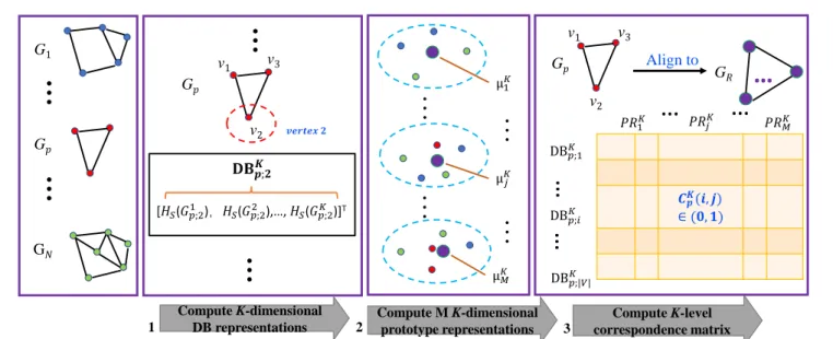
v3 v2 v1 v3 v2 G𝑝 Align toFig. 2. The procedure of computing the correspondence matrix. Given a set of graphs, for each graphGp: (1) we compute theK-dimensional depth-based (DB) representationDBK
p;vrooted at each vertex (e.g., vertex 2) as theK-dimensional vectorial vertex representation, where each elementHs(GKp;2)represents
the Shannon entropy of theK-layer expansion subgraph rooted at vertexv2ofGp[35]; (2) we identify a family ofK-dimensional prototype representations PRK={µK
1, . . . , µKj , . . . , µKM}using k-means on theK-dimensional DB representations of all graphs; (3) we align theK-dimensional DB representations to theK-dimensional prototype representations and compute aK-level correspondence matrixCK
p.
˜
Ap. IfGpare vertex attributed graphs,Xp can be the one-hot encoding matrix of the vertex labels. For un-attributed graphs, we propose to use the vertex degree as the vertex label.
For each graphGp, we utilize the proposed transitive vertex matching method to compute the K-level vertex correspon-dence matrixCK
p that records the correspondence information between the K-dimensional vectorial vertex representation of Gp and the K-dimensional prototype representations in PRK = {µK
1 , . . . , µKj , . . . , µKM}. With CpK to hand, we compute theK-level aligned vertex feature matrix forGp as
¯
XpK = (CpK)TXp, (6)
where X¯pK ∈ RM×c and each row of X¯pK represents the feature of a corresponding aligned vertex. Moreover, we also compute the associatedK-level aligned vertex adjacency matrix forGp as
¯
AKp = (CpK)T( ˜Ap)(CpK), (7) where A¯K
p ∈RM×M. Both X¯pK andA¯Kp are indexed by the corresponding prototypes in PRK. Since X¯pK and A¯Kp are computed from the original vertex feature matrixXp and the original adjacency matrix Ap, respectively, by mapping the˜ original feature and adjacency information of each vertexvp∈ Vpto that of the new aligned vertices,X¯pKandA¯Kp encapsulate the original feature and structural information ofGp. Note that, since each prototype may be aligned by multiple vertices from Vp,A¯K
p may be a weighted adjacency matrix.
In order to construct the fixed-sized aligned grid structure for each graph Gp ∈ G, we need to sort the vertices to determine their spatial orders. Since the vertices of each graph are all aligned to the same prototype representations, we sort the vertices of each graph by reordering the prototype representations. To this end, we construct a prototype graph GR(VR, ER) that captures the pairwise similarity between the K-dimensional prototype representations in PRK, with each vertexvj ∈VRrepresenting the prototype representation µK
j ∈ PR
K
and each edge (vj, vk) ∈ ER representing
the similarity between µK
j ∈ PR
K and µK
k ∈ PR
K. The similarity between two vertices ofGR is computed as
s(µKj , µKk) = exp(−kµ K
j −µKk k2
K ). (8)
The degree of each prototype representationµK
j isDR(µKj ) =
PM
k=1s(µKj , µKk). We propose to sort the K-dimensional prototype representations in PRK according to their degree DR(µKj ). Then, we rearrangeX¯pK andA¯Kp accordingly.
To construct reliable grid structures for graphs, in this work we employ the depth-based (DB) representations as the vec-torial vertex representations to compute the requiredK-level vertex correspondence matrixCpK. The DB representation of each vertex is defined by measuring the entropies on a family of k-layer expansion subgraphs rooted at the vertex [36], where the parameter k varies from 1 to K. It is shown that such a K-dimensional DB representation encapsulates rich entropy content flow from each local vertex to the global graph structure, as a function of depth. The process of computing the correspondence matrix CK
p associated with depth-based representations is shown in Fig.3. When we vary the number of layersKfrom1toL(i.e.,K≤L), based on the definition in our previous work [33], we compute the finalaligned vertex grid structurefor each graph Gp∈Gas
¯ Xp= L X K=1 ¯ XpK L , (9)
and the associated aligned grid vertex adjacency matrix as ¯ Ap= L X K=1 ¯ AKp L , (10)
where Xp¯ ∈ RM×c, Ap¯ ∈ RM×M, the i-th row of Xp¯
corresponds to the feature vector of thei-th aligned grid vertex, and thei-row andj-column element ofAp¯ corresponds to the adjacent information between thei-th and j-th grid vertices.
Note that, the adjacency matrix A¯p corresponds to an undirected graph. Directly associating this matrix with existing spatial graph convolution operations may also suffer from tottering problems, since the vertex feature information may be propagated from the starting vertex to a vertex through an undirected edge (i.e., a bidirectional edge) and then immedi-ately propagated back to the starting vertex through the same edge. This in turn results redundant feature information, and influences the performance of existing spatially-based GCN models. To address this problem, we propose to transformAp¯ into a backtrackless adjacency matrix A¯Dp, that correspond-s to a directed graph. More formally, with the undirected aligned vertex adjacency matrix A¯D
p to hand, we commence by computing the degree of each i-th aligned grid vertex as
¯ DD p(i) = P jA¯ D
p(i, j). The probability of the classical steady state random walk visiting thei-th vertex is then computed as
P(i) = ¯DDp(i)/X j
¯
DpD(j). (11)
We compute the backtrackless aligned grid vertex ad-jacency matrix A¯D
p of each graph Gp by replacing each bidirectional edge residing onA¯pas a directed edge associated with the visiting probabilities of classical random walks, i.e.,
¯
ADp(vi, vj) =
¯
Ap(vi, vj) if P(i)6P(j),
0 otherwise. . (12)
whereviandvj are thei-th andj-th aligned grid vertices, and P(i) and P(j) are the probabilities of the classical random walk visitingvi andvj. Clearly,A¯Dp corresponds to a directed graph. Unlike the undirected grid vertex adjacency matrix
¯ AD
p, the backtrackless grid vertex adjacency matrix A¯Dp is not a symmetric matrix. If the i-row and j-column element of A¯D
p is greater than0, we say that there is a directed edge from the grid vertex vi to the grid vertex vj. Since, the vertex feature information cannot immediately propagate back to the starting vertex along a directed edge within the spatial graph convolution operation, A¯D
p provides a natural backtrackless structure to restrict the tottering problem. Finally, note that, Eq.(12) will not change the trace of Ap¯ that encapsulates the self-loop information residing on the original self-looped adjacency matrix A˜ofGp. Thus,A¯D p cannot restrict the tottering problem of each original vertex itself. This is because each vertex will constantly propagate its own information to itself along its self-loop connection during the convolution operation. To overcome this problem, we propose to remove the added self-loops of A˜ before we compute A¯D
p through Eq.(12). As a result, each vertex can only propagate its own information to itself through its neighboring vertices, restricting the self tottering problem. Remark: Eq.(9) and Eq.(12) indicate that they can transform the original graph Gp ∈Gwith arbitrary number of vertices |Vp|into a new backtrackless aligned grid graph structure with the same number of vertices, where Xp¯ is the corresponding aligned grid vertex feature matrix andA¯Dp is the corresponding backtrackless aligned grid vertex adjacency matrix. Since both
b
Xp andA¯Dp are mapped through the original graph Gp, they not only reflect reliable structure correspondence information
betweenGpand the remaining graphs in graph setGbut also encapsulate more original feature and structural information of Gp. Furthermore, since the orientation of each directed edge residing on the backtrackless adjacency matrix A¯D
p is from a vertex with a lower visiting probability of random walks to that with a higher visiting probability of random walks,A¯D p encapsulates rich visiting information of random walks. 2
IV. THEBACKTRACKLESSALIGNED-SPATIALGRAPH
CONVOLUTIONALNETWORKMODEL
In this section, we propose a new spatially-based GCN mod-el, i.e., the Backtrackless Aligned-Spatial Graph Convolutional Network (BASGCN) model. The core stage of a spatially-based GCN model is the associated graph convolution opera-tion that extracts multi-scale features for each vertex based on the original features of its neighbour vertices as well as itself. As we have stated, most existing spatially-based GCN models perform the convolution operation by first applying a trainable parameter matrix to map the original feature of each vertex inc dimensions to that in c0 dimensions, and then averaging the vertex features of specified vertices [25], [26], [27], [31]. Since the trainable parameter matrix is shared by all vertices, these models cannot discriminate the importance of different vertices and have inferior ability to aggregate vertex features. Moreover, as we have indicated, most existing spatially-based GCN models are theoretically related to the classical WL algorithm [11], and the required convolution operation of these GCN models relies on the vertex feature propagation between each vertex and its neighboring vertices [25], [26], [27], [31]. Thus, similar to the WL algorithm, these WL analogous GCN models may propagate the feature information from the starting vertex to a vertex and then immediately propagate the information back to the starting vertex, resulting in redun-dant feature information. To overcome these shortcomings, in this section we first propose a new backtrackless spatial graph convolution operation associated with the backtrackless aligned grid structures of graphs. Unlike existing methods, the trainable parameters of the proposed convolution operation can directly influence the aggregation of the aligned grid vertex features, thus the proposed convolution operation can discriminate the importance between specified aligned grid vertices. Furthermore, since the process of the vertex feature information propagation relies on the backtrackless aligned grid vertex adjacency matrix, the proposed convolution opera-tion can significantly reduce the tottering problem. Finally, we introduce the architecture of the BASGCN model associated with the proposed convolution operation.
A. The Backtrackless Spatial Graph Convolution Operation
In this subsection, we propose a family of backtrackless spatial graph convolution operations to further extract multi-scale features of graphs, by propagating features between aligned grid vertices through the backtrackless aligned grid vertex adjacency matrix. Specifically, given a sample graph G(V, E) with its aligned vertex grid structure X¯ ∈ RM×c
and the associated backtrackless aligned grid vertex adjacency matrix A¯D ∈
spatial graph convolution operations consist of an in-spatial convolution as well as an out-spatial convolution and take the forms as Zinh = Relu( ¯Din−1A¯in c X j=1 ( ¯XWh)[:,j]), (13) and
Zouth = Relu( ¯Dout−1A¯out c
X
j=1
( ¯XWh)[:,j]), (14)
whererepresents the element-wise Hadamard product,A¯in equals to ( ¯AD)T and is thein-adjacency matrix(i.e., for the i-th row, its j-th column elements of A¯in correspond to the directed edges to the i-th grid vertex from these j-th grid vertices, and we regard these j-th grid vertices as the in-neighboring vertices of thei-th grid vertex),A¯out equals to
¯
ADand is theout-adjacency matrix(i.e., for thei-th row, its j-th column elements ofA¯outcorrespond to the directed edges from the i-th grid vertex to these j-th grid vertices, and we regard thesej-th grid vertices as theout-neighboring vertices of the i-th grid vertex),D¯in is the in-degree matrixof A¯in,
¯
Dout is the out-degree matrix of A¯out. More specifically, Eq.(13) corresponds to the in-spatial graph convolution operation(i.e., for each grid vertex this convolution operation focuses on propagating the feature information between itself and its in-neighboring vertices). Eq.(14) corresponds to the out-spatial graph convolution operation (i.e., for each grid vertex this convolution operation focuses on propagating the feature information between itself and its out-neighboring vertices). The in-spatial and out-spatial convolution operations share the same trainable parameter matrix Wh ∈ RM×c for
both theirh-th convolution filters with the filter sizeM×1and the channel numberc.Reluis the rectified linear units function (i.e., a nonlinear activation function), and Zh
in ∈ RM×1 and Zh
out ∈ RM×1 are the output activation matrices for the in-spatial and out-in-spatial convolution operations.
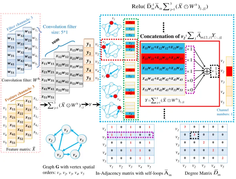
An instance of the proposed in-spatial graph convolution operation defined by Eq.(13) is shown in Fig.3. Specifically, this convolution operation consists of four steps. In the first step, the procedurePc
j=1( ¯XW h)
[:,j] commences by computing the element-wise Hadamard product between X¯ and Wh, and then summing the channels of X¯ Wh (i.e., summing the columns ofX¯Wh). Fig.3 exhibits this process. Assume X¯ is the collection of 5 aligned grid vertex feature vectors in the 3 dimensions (i.e., 3 feature channels), Wh is the h-th convolution filter with the filter size 5 ×1 and the channel number 3. The resulting P3
j=1( ¯XW h)
[:,j] first assigns the feature vector x[i,:] of each i-th aligned grid vertex a different weighted vector w[i,:], and then sums the channels of each weighted feature vector. For the first step,
Pc
j=1( ¯XWh)[:,j] can be seen as a new weighted aligned vertex grid structure with1vertex feature channel.The second stepA¯inY, whereY :=P
c
j=1( ¯XW h)
[:,j], propagates the weighted feature information between each aligned grid vertex as well as its in-neighboring aligned grid vertices. Specifically, each i-th row( ¯AinY)[i,:] ofA¯inY equals to PjA¯in;[i,j]Y[:,j], and can be seen as the aggregated feature vector of the i-th
aligned grid vertex by summing its original weighted feature vector as well as all the original weighted feature vectors of the j-th aligned grid vertex that has a directed edge to it (i.e., its in-neighboring vertices). Note that, since the first step has assigned each i-th aligned grid vertex a different weighted vector w[i,:], this aggregation procedure is similar to performing a standard fixed-sized convolution filter on a standard grid structure, where the filter first assigns different weighted vectors to the features of each grid element as well as its neighboring grid elements and then aggregates (i.e., sum) the weighted features as the new feature for each grid element. This indicates that the trainable parameter matrix Wh of the proposed convolution operation can directly influence the aggregation process of the vertex features, i.e., it can adaptively discriminate the importance between specified in-neighboring vertices. Fig.3 exhibits this propagation process. For the 2-nd aligned grid vertex v2 (marked by the red broken-line frame), the 1-st and 3-rd aligned grid verticesv1 andv3are its in-neighboring vertices. The process of computing P
jA¯in;[2,j]Y[:,j] (marked by the red real-line frame) aggregates the weighted feature vectors of aligned grid vertexv2as well as its in-neighboring aligned grid vertices v1 andv3 as the new feature vector of v2. The vertices participating in this aggregation process are indicated by the 2-nd row of A¯in (marked by the purple broken-line frame on A) that encapsulates the in-adjacent information¯ of aligned grid vertices. The third step normalizes each i-th row of A¯inY by multiplying D¯in;[−1i,i], where D¯in;[i,i] is the i-th diagonal element of the in-degree matrix D¯in. This process can guarantee a fixed feature scale after the proposed convolution operation. Specifically, Fig.3 exhibits this normalization process. The aggregated feature of the 2 -nd aligned grid vertex (marked by the red real-line frame) is multiplied by 3−1, where 3 is the 3-rd diagonal element of
¯
Din (marked by the black broken-line frame on D¯in). The
last step employs the Relu activation function and outputs the convolution result. Note that, since the proposed in-spatial graph convolution operation defined by Eq.(13) only extracts new features for the aligned grid vertex and does not change the orders of the aligned vertices, the output Zinh is still an aligned vertex grid structure with the same vertex order ofX¯. Similar to the in-spatial graph convolution operation, the out-spatial graph convolution operation defined by Eq.(14) can also be explained by Fig.3, by replacing both the in-adjacency matrix A¯in and the in-degree matrix D¯in as the out-adjacency matrix A¯out and the out-degree matrix D¯out. As a result, different from the in-spatial graph convolution operation, the out-spatial graph convolution operation focuses on propagating the weighted feature information between each aligned grid vertex as well as its out-neighboring aligned grid vertices. Moreover, the output Zh
out of the out-spatial convolution operation is also an aligned vertex grid structure with the same vertex order ofX.¯
Finally, the above theoretical explanation indicates that both the in-spatial and out-spatial graph convolution operations can significantly reduce the drawback of tottering problems, that arises in mosting existing spatially-based GCN models [25],
Convolution filter size: 5*1 3 h :, j j 1= (X W )
v1 v2 v5 v3 v4Graph Gwith vertex spatial orders: v1, v2, v3, v4, v5 v2 v1 v3 v4 v5 x11w11+x12w12+x13w13 x21w21+x22w22+x23w23 x31w31+x32w32+x33w33 x41w41+x42w42+x43w43 x51w51+x43w43+x53w53
0 0 1 1 0 1 0 1 1 1 1 0 0 0 0 1 0 1 0 0 1 1 0 0 0 0 1 1 v3 v4 v5 v2 v1 v2 v3 v4 v5In-Adjacency matrix with self-loops
3 0 0 0 0 0 3 0 0 0 0 0 2 0 0 0 0 0 2 0 0 0 0 0 2 v3 v4 v5 v2 v1 v2 v3 v4 v5 Degree Matrix v1 v3 v4 v5 v2 Channel numbers: 1
...
....
. 3 -1 in in j 1 [:, j]Relu( D A
=(
X
W
h)
)
Concatenation of v
2: v1 v1 inA
D
in 1 3 1 1 in;[ 2, ] j] jA
jY
[:, v1 v3 v5 v1 v2 v3 v3 v5 v3 v4 v4 v5 3 h [:, j] j 1 = ( ) Y
= X W 𝒘𝟏𝟑 𝒘𝟐𝟑 𝒘𝟑𝟑 𝒘𝟒𝟑 𝒘𝟓𝟑 𝒘𝟏𝟐 𝒘𝟐𝟐 𝒘𝟑𝟐 𝒘𝟒𝟐 𝒘𝟓𝟐 𝒘𝟏𝟏 𝒘𝟐𝟏 𝒘𝟑𝟏 𝒘𝟒𝟏 𝒘𝟓𝟏 𝒙𝟏𝟑 𝒙𝟐𝟑 𝒙𝟑𝟑 𝒙𝟒𝟑 𝒙𝟓𝟑 𝒙𝟏𝟐 𝒙𝟐𝟐 𝒙𝟑𝟐 𝒙𝟒𝟐 𝒙𝟓𝟐 𝒙𝟏𝟏 𝒙𝟐𝟏 𝒙𝟑𝟏 𝒙𝟒𝟏 𝒙𝟓𝟏 v5 v4 v3 v2 v1 x5,: x4,: x3,: x2,: x1,: w5,: w4,: w3,: w2,: w1,: Feature matrix: 𝑋ത Convolution filter: 𝑊ℎ 𝒙𝟏𝟑𝒘𝟏𝟑 𝒙𝟐𝟑𝒘𝟐𝟑 𝒙𝟑𝟑𝒘𝟑𝟑 𝒙𝟒𝟑𝒘𝟒𝟑 𝒙𝟓𝟑𝒘𝟓𝟑 𝒙𝟏𝟐𝒘𝟏𝟐 𝒙𝟐𝟐𝒘𝟐𝟐 𝒙𝟑𝟐𝒘𝟑𝟐 𝒙𝟒𝟐𝒘𝟒𝟐 𝒙𝟓𝟐𝒘𝟓𝟐y
1y
2y
3y
4y
5 𝒙𝟏𝟏𝒘𝟏𝟏 𝒙𝟐𝟏𝒘𝟐𝟏 𝒙𝟑𝟏𝒘𝟑𝟏 𝒙𝟒𝟏𝒘𝟒𝟏 𝒙𝟓𝟏𝒘𝟓𝟏 v5 v4 v3 v2 v1 YFig. 3. An Instance of the Proposed Backtrackless In-Spatial Graph Convolution Operation.
[26], [27] theoretically related to the WL algorithm [11]. This is because both the convolution operations are defined by propagating vertex feature information through the back-trackless aligned grid vertex adjacency matrix (i.e., the in and our adjacency matrices A¯in andA¯out), that corresponds to a directed graph. Thus, the vertex feature information cannot be immediately propagated back to the starting vertex through a directed edge within the spatial graph convolution operation. In other words, the current convolution operation can propagate the vertex feature information from a starting vertex to a vertex along (for the in-convolution) or against (for the out-convolution) a directed edge, but the next convolution operation cannot immediately propagate the information back from the vertex to the starting vertex against (for the in-convolution) or along (for the out-in-convolution) the same directed edge. As a result, both the in-spatial and out-spatial graph convolution operations are Backtrackless Spatial Graph Convolution Operations.
B. The Architecture of the Proposed BASGCN Model
We introduce the architecture of the proposed BASGCN model, that has been shown in Fig.1. Specifically, the architecture is composed of three sequential stages, i.e., 1)
the backtrackless grid structure construction/input layer, 2) the backtrackless spatial graph convolution layer, and 3) the traditional One-dimensional CNN layers.
The Backtrackless Grid Structure Construction/Input Layer: For the proposed BASGCN model, we commence by employing the transitive vertex matching method defined earlier to convert each graph G ∈ G of arbitrary sizes into the fixed-sized backtrackless aligned grid structure, including the aligned vertex grid structure X¯ as well as the associated backtrackless aligned grid vertex adjacency matrix A. Then,¯ we pass the grid structures to the proposed BASGCN model. The Spatial Graph Convolutional Layer: For each graph G, to extract multi-scale features of the aligned grid vertices, we define a pair of paralleling stacked multiple backtrackless graph convolution layers associated with the proposed in-spatial and out-in-spatial graph convolution operations respec-tively, i.e., theIn-BASGCNnetwork focusing on aggregating vertex features of itself and its in-neighboring vertices and the Out-BASGCN network focusing on aggregating vertex features of itself and its out-neighboring vertices (see Fig.1 for details). Both networks are backtrackless GCNs. More formally, the In-BASGCN network associated with Eq.(13)
and the Out-BASGCN network associated with Eq.(14) are separately defined as Zin;ht= Relu( ¯D−in1A¯ Ht−1 X j=1 (Zin;t−1Wth)[:,j]), (15) and Zout;h t= Relu( ¯D− 1 outA¯ Ht−1 X j=1 (Zout;t−1Wth)[:,j]), (16)
whereZin;0 andZout;0 are the same and equal to the aligned vertex grid structure X, Eq.(15) and Eq.(16) correspond to¯ the stacked In-BASGCN and Out-BASGCN networks and share the same trainable parameters, Ht−1 is the number of convolution filters in the (t −1)-th graph convolution layer for the stacked In-BASGCN or Out-BASGCN network, Zin;t−1 ∈ RM×Ht−1 and Zout;t−1 ∈ RM×Ht−1 are the
concatenated outputs of all theHt−1 convolution filters in the
(t−1)-th graph convolution layer of the stacked In-BASGCN and Out-BASGCN networks, Zh
in;t andZout;h t are the outputs of the h-th convolution filter in layer t of the stacked In-BASGCN and Out-In-BASGCN networks, and Wh
t ∈RM×Ht−1 is the trainable parameter matrix of the h-th convolution filter in layer t with the filter sizeM ×1 and the channel number Ht−1for the stacked In-BASGCN or Out-BASGCN networks.
The Traditional One-dimensional CNN Layer: For the In-BASGCN and Out-BASGCN networks, we horizontally concatenate the outputs Zin;t and Zout;t of their each t-th spatial graph convolution layers associated with the outputs of their previous1 to(t−1)-th spatial graph convolution layers as well as their original inputsZin;0andZout;0asZin;(0:t)and Zout;(0:t), i.e.,Zin;(0:t)= [Zin;0, Zin;1, . . . , Zin;t]andZin;0:t∈
RM×(c+ Pt
z=1Ht), andZ
out;(0:t)= [Zout;0, Zout;1, . . . , Zout;t] and Zout;0:t ∈ RM×(c+
Pt
z=1Ht). As a result, for the con-catenated outputs Zin;0:t andZout;0:t, each of their rows can be seen as the new multi-scale features for the corresponding aligned grid vertex. Since both Zin;0:t and Zout;0:t are still aligned vertex grid structures, one can directly utilize the tradi-tional CNN on these grid structures. Specifically, Fig.1 exhibits the architecture of a pair of paralleling traditional CNN layers, where the upper CNN layers are associated with each Zin;0:t of the In-BASGCN network, and the lower CNN layers are associated with each Zout;0:t of the Out-BASGCN network. Similar to the In-BASGCN and Out-BASGCN networks, both the upper and lower CNN layers also share the same trainable parameters. Moreover, each concatenated vertex grid structure Zin;0:t or Zout;0:t can be seen as aM ×1 (in Fig.1 M = 5) vertex grid structure and each vertex is represented by a (c+Pt
z=1Ht)-dimensional feature, i.e., the channel of each grid vertex isc+Pt
z=1Ht. Then, we add a one-dimensional convolution layer for each Zin;0:tor Zout;0:t. The convolution operation can be performed by sliding a fixed-sized filter of size k×1 (in Fig.1 k = 3) over the spatially neighboring vertices. After this, several AvgPooling layers and remaining one-dimensional convolution layers can be added to learn the local patterns on the aligned grid vertex sequence. Finally,
when we varytfrom0toT (in Fig.1T = 2), we will obtain T+ 1extracted pattern representations for the upper or lower CNN layers. We concatenate the extracted patterns of each Zin;0:torZout;0:tand add a fully-connected layer. A Softmax layer is added and follows the fully-connected layers of both the upper and lower CNN layers.
C. Discussions and Related Works
Comparing to existing state-of-the-art spatial graph convo-lution network models, the proposed BASGCN model has a number of advantages.
First, in order to transform the extracted multi-scale features from the graph convolution layers into fixed-sized representa-tions, both the Neural Graph Fingerprint Network (NGFN) model [26] and the Diffusion Convolution Neural Network (DCNN) model [25] sum up the extracted local-level vertex features as global-level graph features through a SumPooling layer. Although the fixed-sized features can be directly read by a classifier for classifications, it is difficult to capture local topological information residing on the local vertices through the global-level graph features. By contrast, the pro-posed BASGCN model focuses more on extracting local-level aligned grid vertex features through the proposed backtrackless spatial graph convolution operations (i.e., the in-spatial and the out-spatial graph convolution) on the aligned grid structures of graphs. Thus, the proposed BASGCN model can encapsulate richer local structural information than the NGFN and DCNN models associated with SumPooling.
Second, similar to the proposed BASGCN model, both the PATCHY-SAN based Graph Convolution Neural Network (PSGCNN) model [32] and the Deep Graph Convolution Neural Network (DGCNN) model [31] also need to form fixed-sized vertex grid structures for arbitrary-sized graphs. To achieve this, these models rearrange the vertex order of each graph structure, and preserve a specified number of vertices with higher ranks. Although, unify the number of vertices for different graphs, the discarded vertices may lead to significant information loss. By contrast, the associated aligned grid structures of the proposed BASGCN model can encapsulate all the original vertex features from the original graphs, thus the proposed BASGCN model constrains the shortcoming of information loss arising in the PSGCNN and DGCNN models. On the other hand, both the PSGCNN and DGCNN models tend to sort the vertices of each graph based on the local struc-tural descriptor, ignoring consistent vertex correspondence in-formation between different graphs. By contrast, the associated backtrackless aligned grid structure of the proposed BASGCN model is constructed through a transitive vertex alignment procedure. As a result, only the proposed BASGCN model can encapsulate the structural correspondence information between any pair of graph structures, i.e., the vertices on the same spatial position are also transitively aligned to each other.
Third, as we have stated in Sec.IV-A, both the backtrackless in-spatial and out-spatial graph convolution operations of the proposed BASGCN model are similar to performing standard fixed-sized convolution filters on standard grid structures. To further reveal this property, we utilize the in-spatial graph
convolution operation as a typical instance and explain the convolution process one step further associated with Fig.3. For the sample graph Gshown in Fig.3, assume it has 5 vertices following the fixed spatial vertex orders (positions)v1,v2,v3, v4 and v5, X¯ is the collection of its vertex feature vectors with 3 feature channels, and Wh is the h-th convolution filter with the filter size 5 ×1 and the channel number 3. Specifically, the procedure marked by the blue broken-line frame of Fig.3 indicates that performing the proposed spatial graph convolution operation associated with the in-adjacency matrix on the aligned vertex grid structure X¯ can be seen as respectively performing the same 5 × 1-sized convolution filter Wh on five 5 × 1-sized local-level in-neighborhood vertex grid structures included in the green broken-line frame. Here, each in-neighborhood vertex grid structure only encapsulates the original feature vectors of a root vertex as well as its in-adjacent vertices from G (i.e., the vertices having directed edges to the root vertex), and all the vertices follow their original vertex spatial positions in G. For the non in-adjacent vertices, we assign dummy vertices (marked by the grey block) on the corresponding spatial positions of the in-neighborhood vertex grid structures, i.e., the elements of their feature vectors are all 0. Since the five in-neighborhood vertex grid structures are arranged by the spatial orders of their root vertices from G, the vertically concatenation of these in-neighborhood vertex grid structures can be seen as a 25×1-sized global-level grid structure X¯G of G. We observe that the process of the proposed in-spatial graph convolution operation on X¯ is equivalent to sliding the 5×1 fixed-sized convolution filter Wh over X¯
G with
5-stride, i.e., this process is equivalent to sliding a standard classical convolution filter on standard grid structures. As a result, the in-spatial graph convolution operation of the proposed BASGCN model is theoretically related to the classical convolution operation on standard grid structures, bridging the theoretical gap between traditional CNN models and the spatially-based GCN models. Note that, we will obtain the same analysis result, if we utilize the out-spatial graph convolution operation as the typical instance.
Fourth, the above third observation indicates that both the in-spatial and out-spatial graph convolution operations are theoretically related to the classical convolution operation, and can assign each vertex a different weighted parameter. Thus, the proposed BASGCN model associated with the in-spatial and out-spatial graph convolution operations can adaptively discriminate the importance between specified in-neighboring or out-neighboring vertices during the convolution operation. By contrast, as we have stated in Sec.II, the existing spatial graph convolution operation of the DGCNN model only maps each vertex feature vector in c dimensions to that in c0 dimensions, and all the vertices share the same trainable parameters. As a result, the DGCNN model has less ability to discriminate the importance of different vertices during the convolution operation.
Fifth, as we have stated in Sec.II, most existing spatially-based GCN models (e.g., the DGCNN, NGFN and DCNN, models) are theoretically related to the classical WL algo-rithm [11]. Similar to the WL algoalgo-rithm, these GCN models
suffer from tottering problem. This is because the associated graph convolution operations of these GCN models rely on the vertex feature information propagation through the undirected edges. As a result, they may propagate the feature information from the starting vertex to a vertex and then immediately propagate the information back to the starting vertex through the same undirected edge. By contrast, the proposed BASGCN model is defined based on the backtrackless aligned grid structure that corresponds to a directed graph rather than an undirected graph. The associated in-spatial or out-spatial graph convolution operations cannot immediately propagate the vertex feature information against or along the directed edge. Thus, the proposed BASGCN model can significantly reduce the tottering problem arising in existing spatially-based GCN models.
Finally, similar to the proposed BASGCN model, the orig-inal ASGCN model [33] cannot only reduce the information loss arising in most existing GCN models, but also bridge the theoretical gap between the traditional CNN models and spatially-based GCN models. This is because the ASGCN model is also based on the aligned grid structure computed based on the transitive vertex alignment method. However, similar to existing spatially-based GCN models, the original ASGCN model also suffers from the tottering problem. This is because, unlike the proposed BASGCN model, the associated spatial graph convolution operation of the ASGCN model is defined through the undirected grid vertex adjacency matrix (i.e., it is not defined on a backtrackless structure). By contrast, the proposed BASGCN model is based on the backtrackless aligned grid structure, and can extract two kinds of multi-scale vertex features for each vertex though both the in-spatial and out-spatial graph convolution operations, thus reflecting richer graph characteristics than the original ASGCN model. Finally, note that, both the in-spatial and out-spatial graph convolu-tion operaconvolu-tions share the same trainable parameters. Thus, for the proposed BASGCN model, its associated in-spatial and out-spatial graph convolution operations are theoretically equivalent, if we replace the backtrackless grid structure as the backtracked grid structure used in the ASGCN model. Then, the BASGCN model will be as the same as the original ASGCN model, indicating that the proposed BASGCN model can generalize the original ASGCN model. As a result, the proposed BASGCN model not only inherits all the ad-vantages of the original ASGCN model, but also further generalizes the original model as a new backtrackless model to reduce the tottering problem and reflect richer graph characteristics.
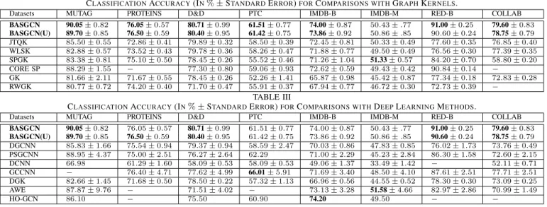
V. EXPERIMENTS
In this section, we evaluate the performance of the proposed BASGCN model, and compare it to both state-of-the-art graph kernels and deep learning methods on graph classification problems. Specifically, the classification is evaluated with eight standard graph datasets abstracted from bioinformatics and social networks. Details of these datasets are shown in Table.I.