Solving Large-Scale Multi-Objective Optimization Problems with Sparse Optimal Solutions via Unsupervised Neural Networks

Solving Large-Scale Multi-Objective

Optimization Problems with Sparse Optimal

Solutions via Unsupervised Neural Networks

Ye Tian, Chang Lu, Xingyi Zhang,

Senior Member, IEEE

, Kay Chen Tan,

Fellow, IEEE

,

and Yaochu Jin,

Fellow, IEEE

Abstract—Due to the curse of dimensionality of search space, it is extremely difficult for evolutionary algorithms to approximate the optimal solutions of large-scale multi-objective optimization problems (LMOPs) by using a limited budget of evaluations. If the Pareto optimal subspace is approximated during the evolutionary process, the search space can be reduced and the difficulty encountered by evolutionary algorithms can be highly alleviated. Following the above idea, this paper proposes an evolutionary algo-rithm to solve sparse LMOPs by learning the Pareto optimal subspace. The proposed algorithm uses two unsupervised neural networks, a restricted Boltzmann machine and a denoising autoencoder to learn a sparse distribution and a compact representation of the decision variables, where the combination of the learnt sparse distribution and compact representation is regarded as an approximation of the Pareto optimal subspace. The genetic operators are conducted in the learnt subspace, and the resultant offspring solutions then can be mapped back to the original search space by the two neural networks. According to the experimental results on eight benchmark problems and eight real-world problems, the proposed algorithm can effectively solve sparse LMOPs with 10,000 decision variables by only 100,000 evaluations.

Manuscript received –. This work was supported in part by the National Key Research and Development Project under Grant 2018AAA0100105, in part by the National Natural Science Foundation of China under Grant 61672033, Grant 61822301, Grant 61876123, Grant 61906001, and Grant U1804262, in part by the Hong Kong Scholars Pro-gram under Grant XJ2019035, in part by the Anhui Provincial Natural Science Foundation under Grant 1808085J06 and Grant 1908085QF271, in part by the State Key Laboratory of Synthetical Automation for Process Industries under Grant PAL-N201805, and in part by the Research Grants Council of the Hong Kong Special Administrative Region, China under Grant CityU11202418 and Grant CityU11209219, (Corresponding author: Xingyi Zhang.)

Y. Tian is with the Key Laboratory of Intelligent Computing and Signal Processing of Ministry of Education, Institutes of Physical Science and Information Technology, Anhui University, Hefei 230601, China, and also with the Department of Computer Science, City University of Hong Kong, Kowloon Tong, Hong Kong SAR (email: [email protected]).

C. Lu and X. Zhang are with the Key Laboratory of Intelligent Computing and Signal Processing of Ministry of Education, School of Computer Science and Technology, Anhui University, Hefei 230601, China (email: lucy [email protected]; [email protected]).

K. C. Tan is with the Department of Computer Science, City University of Hong Kong, Kowloon Tong, Hong Kong SAR (email: [email protected]).

Y. Jin is with the Department of Computer Science, University of Surrey, Guildford, Surrey, GU2 7XH, U.K., and also with the Department of Computer Science and Engineering, Southern Uni-versity of Science and Technology, Shenzhen 518055, China (email: [email protected]).

Index Terms—Large-scale multi-objective optimization, sparse Pareto optimal solutions, Pareto optimal subspace, restricted Boltzmann machine, denoising autoencoder

I. INTRODUCTION

I

com-plicated data in many research fields and real-world applications, which raises a variety of optimization prob-lems having multiple objectives and a large number of decision variables [1]–[3]. These large-scale multi-objective optimization problems (LMOPs) present a huge search space that grows exponentially with the number of decision variables, posing stiff challenges for evolu-tionary algorithms to efficiently approximate the Pareto optimal solutions [4]. To address the inevitable “curse of dimensionality”, some multi-objective evolutionary algorithms (MOEAs) have been tailored for LMOPs, which are mainly based on the following two ideas.

The first idea for solving LMOPs is decision variable decomposition, which adopts the divide-and-conquer strategy that divides the decision variables into several groups randomly or heuristically, and optimizes each group of decision variables separately. For example, NSCCGA [5] relates each decision variable to a subpop-ulation, then optimizes each subpopulation by NSGA-II [6]. MOEA/DVA [7] divides the decision variables into position variables, distance variables, and mixed variables, and further divides the distance variables according to their interactions on the objective functions. MOEA/DVA first optimizes each group of distance vari-ables until the population converges, then fine-tunes all the decision variables for better diversity. LMEA [8] clusters the decision variables into convergence-related variables and diversity-related variables, and iteratively optimizes each type of variables by different strategies.

The second idea for solving LMOPs is problem trans-formation, which aims to convert the original LMOP into a small-scale problem, so that it can be handled by general optimizers. Different from traditional decompo-sition based MOEAs (e.g., those based on hierarchical decomposition [9] or Minkowski distance [10]) using a set of weights to transfer multi-objective optimization into single-objective optimization, WOF [11] uses a set

of weights to alter the decision variables, where each weight is related to multiple decision variables and the number of weights is much smaller than the number of decision variables. As a result, a small-scale problem can be established by considering the weights as vari-ables to be optimized. LSMOF [12] defines two reference directions on a solution in search space, and searches for better solutions by moving the solutions along the reference directions. In other words, better solutions can be found by optimizing only two weights, where each weight determines the location of the solution in a reference direction.

In spite of the promising performance of these MOEAs on some LMOPs, most of them are shown to be of low efficiency or effectiveness [13]. For the decision variable decomposition based MOEAs, a large number of function evaluations are required for detecting the in-teractions between decision variables, and the detecting results are probably inaccurate on functions with compli-cated landscapes [8]. The problem transformation based MOEAs are more vulnerable to getting trapped in local optimums due to the loss of diversified search directions [12], though they can quickly find well-converged solu-tions by optimizing a small-scale problem.

According to the Karush-Kuhn-Tucker condition [14], the Pareto optimal solutions of an LMOP constitute

an(M−1)-dimensional piecewise continuous manifold,

where M is the number of objectives and usually much

smaller than the number of decision variables. That is, all

the Pareto optimal solution can fill a(M−1)-dimensional

Pareto optimal subspace, which accounts for a tiny

pro-portion of the originalD-dimensional search space since

M ≪D. Therefore, the original search space is reducible

if some quasi-optimal solutions have been found, and the difficulty of LMOPs can be highly alleviated. In fact, this regularity property has been essential for many estimation of distribution algorithms [15], [16]. Never-theless, these algorithms still encounter difficulties in solving LMOPs [13], [16], since the interactions between decision variables are so complex that it is difficult to learn the accurate Pareto optimal subspace.

In this paper, we propose a Pareto optimal subspace learning based evolutionary algorithm for solving the LMOPs whose Pareto optimal solutions are sparse, i.e., most decision variables of the Pareto optimal solutions are zero. Such LMOPs widely exist in many real-world applications [17]–[19], but there does not exist any MOEA tailored for them so far. Specifically, the proposed algorithm, termed MOEA/PSL, includes the following two main contributions:

1) The restricted Boltzmann machine (RBM) [20] and denoising autoencoder (DAE) [21] are adopted in the proposed MOEA/PSL to learn the Pareto op-timal subspace. At the beginning of each genera-tion, the decision variables of the non-dominated solutions are used to train the two neural net-works, where the RBM is used to learn a sparse distribution of the decision variables and the DAE

is used to learn a compact representation. The combination of the sparse distribution and compact representation is regarded as an approximation of the Pareto optimal subspace, where genetic opera-tors are conducted in the learnt subspace instead of the original search space. Therefore, the original search space is highly reduced.

2) A parameter adaptation strategy is designed to automatically determine the parameters in Pareto optimal subspace learning. On one hand, the size of hidden layers of the two neural networks is estimated according to the sparsity of the non-dominated solutions. On the other hand, the ra-tio of offspring solura-tions generated in the learnt subspace is dynamically adjusted according to the number of successful offspring solutions generated at the previous generations. This way, the proposed algorithm can adapt to different sparse LMOPs without any predefined parameter.

The rest of this paper is organized as follows. In Section II, an introduction to the sparse LMOPs in real-world applications is given, and existing Pareto optimal subspace learning approaches are reviewed. Section III presents the proposed MOEA/PSL in detail. In Sec-tion IV, the experimental results are presented and ana-lyzed. Finally, conclusions are drawn and future work is outlined in Section V.

II. RELATEDWORK

A. Sparse LMOPs in Real-World Applications

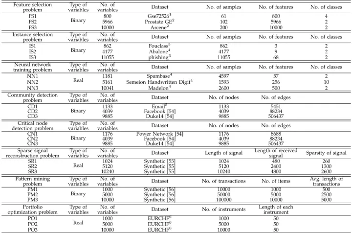
As listed in Table I, sparse LMOPs widely exist in many fields including machine learning, network sci-ence, software engineering, signal processing, data min-ing, economics, and so on. As presented in the table,

these sparse LMOPs contain 10 to 105 _{binary or real}

variables. The binary variable based LMOPs aim to select or delete a small number of elements from a large candi-date set for optimizing specific objectives. For example, the goals of feature selection [17] and instance selection [24] are to select a few features and instances from the training set for the minimum classification error, respectively. Besides, the real variable based LMOPs aim to find the optimal values of a set of parameters, such as the weights in neural network training [37] and the original signal in sparse signal reconstruction [18].

A significant feature of these problems is that their Pareto optimal solutions are sparse. Most of these prob-lems consider the sparsity of solution as an objective to be optimized (e.g., the number of selected features in fea-ture selection, the model complexity in neural network training, and the sparsity of the signal in sparse signal reconstruction), hence the Pareto optimal solutions are sparse. Although some other problems do not explicitly optimize the sparsity of solution, the Pareto optimal solutions are also very sparse due to their objectives. For instance, the community detection problem [38] aims to identify the community centers from all the nodes,

TABLE I

17 SPARSELMOPS INREAL-WORLDAPPLICATIONS.

Field Problem Objectives Type andlength of Meaning of_variables

variables

Machine

Feature selection [22] Minimize the error of the model Binary Whether each feature

Learning

Minimize the number of selected features 13–617 is selected Discretization-based Minimize the error of the model Integer Cut point of feature selection [23] Maximize the diversity of selected features 2308–12600 each feature Instance selection [24] Minimize the error of the model Binary Whether each instance

Minimize the number of selected instances 80–1728 is selected Neural network training [13] Minimize the error of the model Real Weights of the

Minimize the complexity of the model 641–10041 neural network Neural architecture search [25] Minimize the error of the model Binary Architecture of the

Minimize the complexity of the model 4096 neural network

Adversarial attack on Maximize the mislead rates Real Change value of

neural networks [26] Minimize the degree of pixel change 784–120000 each pixel Ensemble learning [27] Minimize the error of the ensemble model Binary Whether each model

Minimize the number of selected models 100 is selected Network

Community detection [28] Maximize the intra-link density Binary Whether each node is Science

Minimize the inter-link density 12–6927 selected as center Critical node detection [29] Minimize the pairwise connectivity Binary Whether each node

Minimize the number of deleted nodes 235–5000 is deleted Influence maximization [30] Maximize the influence Binary Whether each node is

Minimize the cost 5254–15233 selected as seed Minimize the number of deleted features

Software Software product Minimize the number of unused features Binary Whether each feature Engineering configuration [31] Minimize the number of known defects 544–62482 is deleted

Minimize the sum of costs

Signal Sparse signal Minimize the reconstruction error Real _{Reconstructed signal}

Processing reconstruction [18] Minimize the sparsity of the signal 512–10240

Data _{Pattern mining [32]} Maximize the frequency Binary Whether each item

Mining Maximize the completeness 1000–5000 is selected

Economics Portfolio optimization [33] Maximize the expected return Real Portfolio of

Minimize the risk 31–1318 the instruments

Others

Facility location [34] Minimize the facility construction costs Binary Whether each facility Minimize the distance to demand points 2500–105000 is selected Multi-objective knapsack [35] Maximize the profit of each knapsack Binary Whether each item

250–750 is selected

Power grid fault diagnosis [36]

Minimize the difference between

actual and expected states Binary Whether each section Minimize the difference between 28-107 is faulty

observed and actual states

where the number of community centers is much less than the number of nodes; the power grid fault diagnosis problem [39] aims to detect all the faulty sections, which are usually much less than the normal sections.

Although the above problems have been tackled by some MOEAs as listed in Table I, these MOEAs are restricted to the objective functions and data structure of a specific problem, which cannot be used to solve dif-ferent sparse LMOPs in a black-box manner. Therefore, it is necessary to develop a generic MOEAs for solving sparse LMOPs. Besides, existing large-scale MOEAs are inefficient for solving sparse LMOPs due to the compu-tationally expensive objectives. For example, large-scale MOEAs can well solve an LMOP with 5,000 decision variables by using 200,000,000 function evaluations [8], but it is impractical to train a deep neural network for so many times for solving the neural architecture search problem [25]. Considering the sparse nature of Pareto optimal solutions, the Pareto optimal subspace can be approximated by ignoring the dimensions where the decision variables in Pareto optimal solutions are zero. Then, MOEAs can search for better solutions in the learnt subspace instead of the original search space. In other

words, the original search space is drastically reduced. Following this idea, this paper proposes a Pareto op-timal subspace learning based MOEA for solving sparse LMOPs, which will be applied to eight real-world prob-lems selected from Table I. In the next subsection, the Pareto optimal subspace learning approaches in existing MOEAs are reviewed.

B. Existing Pareto Optimal Subspace Learning Approaches

The Pareto optimal subspace learning approaches in existing MOEAs are mainly based on classical machine learning techniques. In [40], two genetic algorithms were proposed for solving MOPs with low effective dimen-sions. The low effective dimensions indicate that the ob-jective functions are only related to a small proportion of the decision variables, hence the Pareto optimal subspace can be easily learnt by ignoring many useless dimen-sions. The algorithms in [40] adopt random embedding to ignore decision variables randomly, which is theoret-ically verified to keep the Pareto optimal subspace un-changed. On the other hand, some MOEAs adopt prin-cipal component analysis (PCA) to learn the Pareto op-timal subspace directly. Based on the condition that the

Pareto optimal solutions lie on an (M −1)-dimensional manifold [14], a regularity model-based multi-objective estimation of distribution algorithm was proposed in

[15]. This MOEA uses an (M −1)-dimensional local

PCA to partition the population into several clusters, and generates offspring solutions around each cluster

centroid. Sun et al. [41] suggested a two-stage MOEA

with Pareto optimal subspace learning, called MaOEA-IT. In the first stage, the algorithm searches for some well-converged solutions by considering only the pop-ulation convergence. In the second stage, it uses these solutions to learn the Pareto optimal subspace via PCA, and generates offspring solutions in the learnt subspace for enhancing the population diversity.

Although the idea of Pareto optimal subspace learning has been successfully adopted in a few MOEAs, they are not suited for solving sparse LMOPs due to the following reasons. Firstly, these approaches learn the Pareto optimal subspace by linearly reducing the de-cision variables, whereas the interactions between the decision variables of many real-world sparse LMOPs are nonlinear. Secondly, these approaches are tailored for specific types of optimization problems, which do not consider the sparse nature of LMOPs. Thirdly, these approaches can only handle continuous decision vari-ables, which are unsuitable for many sparse LMOPs with binary variables.

As reported in [42], a hybrid representation of solu-tion is effective for solving sparse LMOPs, where each solution is represented by a binary vector denoting the mask and a real vector denoting the decision variables. Following this idea, the proposed MOEA/PSL adopts RBM and DAE to learn the Pareto optimal subspace from the solutions with hybrid representation. More specifically, RBM is adopted to learn a sparse distribution from the binary vectors due to its ability of learning the probability distribution of the input obeying a binomial distribution, and DAE is adopted to learn a compact representation from the real vectors due to its ability of learning the compact representation of the input in continuous space. By adopting both RBM and DAE, the proposed MOEA/PSL can control the sparsity of solutions and learn a low-dimensional Pareto optimal subspace, thus highly improving the efficiency in finding sparse and well-converged solutions. In the experiments in Section IV-E, the utilization of both RBM and DAE will be verified by comparing them with a single RBM, DAE, and some other techniques.

In the next subsection, some basic concepts about RBM and DAE are introduced.

C. Restricted Boltzmann Machine (RBM) and Denoising Autoencoder (DAE)

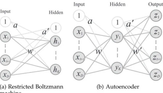
RBM [20] is the building block of deep belief network, which can reduce the dimensionality of input data in an unsupervised manner. As can be seen from Fig. 1(a), a typical RBM consists of an input layer and a hidden

ĉ ĉ Input Hidden

x

x

x

h

h

a

w

a

_’

(a) Restricted Boltzmann machine

w

_’

a

w

x1

x

x

z1

z2

z

z

_a

_’

Fig. 1. General structures of restricted Boltzmann machine and au-toencoder.

layer, where the nodes in the two layers are binary variables obeying a binomial distribution [43]. Given a

vector x as the input, the value of each node hj in the

hidden layer is set to 1 with a probability

p(hj= 1|x) =σ(aj+ Σixiwij), (1)

where aj is the bias, wij is the weight, and σ(x) =

1/(1 + exp(−x)) is the sigmoid function. In practice,

the value of hj is sampled by comparing p(hj = 1|x)

with a uniformly distributed random value within[0,1].

Similarly, the reconstructed value of each nodexi in the

input layer is set to 1 with a probability

p(x′_i= 1|h) =σ(a′_j+ Σjhjwij). (2)

The goal of training RBM is to minimize the reconstruc-tion error (i.e., the difference between the reconstructed

vectorx′and the original inputx) by finding the optimal

values of a, a′ and w, which can be achieved by the

contrastive divergence algorithm [44].

Autoencoder (AE) [45] is the building block of stacked AE, which is also used for dimensionality reduction. Dif-ferent from RBM, AE is a three-layer network working in continuous space. As shown in Fig. 1(b), the value of

each node yj in the hidden layer can be calculated by

yj=σ(aj+ Σixiwij), (3)

and the value of each nodeziin the output layer can be

calculated by

zi=σ(a′i+ Σjyjw′ji). (4)

The reconstruction error of AE is the difference between

the outputzand the inputx, hence AE can be trained by

the same way as feedforward neural network [46]. As for DAE [21], it is a popular variant of AE that enforces the robustness by adding noise to the input. In this work,

each inputx for DAE is perturbed by randomly setting

the elements ofx to zero.

Although the above neural networks have been adopted in estimation of distribution algorithm [47] and evolutionary multitasking algorithm [48], they have not been used in Pareto optimal subspace learning for solving LMOPs before. In this work, RBM and DAE are

/TOZOGRO`GZOUT

3GZOTM YKRKIZOUT

6GXKZU UVZOSGR

Y[HYVGIK MKTKXGZOUT5LLYVXOTM

5LLYVXOTM MKTKXGZOUT

)USHOTGZOUT +T\OXUTSKTZGRYKRKIZOUT

6GXGSKZKXGJGVZGZOUT 3GZOTM YKRKIZOUT 8(3 *'+ 8(3 *'+

Fig. 2. Procedure of MOEA/PSL.

Algorithm 1:Framework of MOEA/PSL

Input:N (population size)

Output:P (final population) 1 P ←Initialization(N);

2 [F1, F2,· · ·]←N ondominatedSorting(P);//Fi is the

set of solutions in the i-th non-dominated

front

3 CrowdDis←CrowdingDistance(F1, F2,· · ·);

4 ρ←0.5;//Ratio of offspring solutions

generated in the Pareto optimal subspace

5 K←N;//Size of the hidden layers

6 whiletermination criterion not fulfilleddo

7 P′←SelectN parents via binary tournament selection according to the non-dominated front number and CrowdDisof solutions inP; 8 O←V ariation(P, P′, ρ, K);

9 P ←P∪O;

10 Delete duplicated solutions fromP; 11 [F1, F2,· · ·]←N ondominatedSorting(P); CrowdDis←CrowdingDistance(F1, F2,· · ·); 12 k←Minimum value s.t.|F1 ∪ · · ·∪Fi| ≥N; 13 Delete|F1 ∪

· · ·∪Fk| −N solutions fromFk with the

smallestCrowdDis; 14 P ←F1 ∪ · · ·∪Fk; 15 [ρ, K]←P arameterAdaptation(P, ρ); 16 returnP;

adopted to learn a sparse distribution and a compact rep-resentation of the decision variables, respectively, where the combination of the learnt sparse distribution and compact representation is regarded as an approximation of the Pareto optimal subspace. In the next section, the procedure of the proposed algorithm is elaborated.

III. THEPROPOSEDALGORITHM

A. Framework of MOEA/PSL

The general framework of MOEA/PSL is presented in

Fig. 2 and Algorithm 1. To begin with, N solutions are

initialized by the Latin hypercube sampling method [49]

to form the initial populationP, and the non-dominated

front number [50] and crowding distance [6] of each

solution are calculated. In the main loop, N parents

are selected by binary tournament selection and used to

generate N offspring solutions. The offspring set O are

then combined with the populationP, and N solutions

with better non-dominated front numbers and crowding

distances in P∪O will survive to the next generation.

Finally, the parameters ρand K are adapted according

to the new population. As a consequence, the mating selection and environmental selection of MOEA/PSL are the same to those of NSGA-II [6], while MOEA/PSL generates some offspring solutions in a learnt subspace. In the following two subsections, the core components of MOEA/PSL are described in detail.

B. Pareto Optimal Subspace Learning and Offspring Gener-ation in MOEA/PSL

The non-dominated solutions in the population are adopted as an approximation of the Pareto optimal solutions for learning the Pareto optimal subspace. To enable RBM and DAE to learn the sparse distribution and compact representation, respectively, each solution

xis represented by a binary vectorxband a real vector

xr, and each decision variable ofxis obtained by

xi=xbi×xri, (5)

wherexbi indicates whether thei-th decision variable is

zero, andxriindicates the real value of thei-th decision

variable. If the problem is with binary variables, the real

vectorxris always set to a vector of ones. In short, each

solution is represented byxbandxrinstead ofx, where

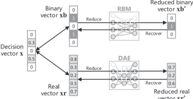
the length of all the three vectors equals to the number of decision variables. Before generating offspring solutions, the binary vectors of all the non-dominated solutions are used to train an RBM via the contrastive divergence algorithm, and the real vectors of all the non-dominated solutions are used to train a DAE via gradient descent. As shown in Fig. 3, the real vector and binary vector of each solution can be reduced by the representation of the hidden layers of the two neural networks, and the reduced vectors can also be recovered to normal vectors. In other words, each solution can be mapped between the original search space and the Pareto optimal subspace, where offspring solutions are generated in the Pareto optimal subspace and evaluated by the objective functions in the original search space.

Afterwards, two parents are randomly picked up from the mating pool each time, whose binary vectors are

*KIOYOUT \KIZUXx (OTGX_ \KIZUXxb 8KGR \KIZUXxr 8(3 *'+ 8KJ[IKJHOTGX_ \KIZUXxb_’ 1 0 0 1 1 0 0 0 0.3 0.5 0.2 0.7 0.8 0.2 0.6 0.7 0.3 0.5 0 0 0 8KJ[IKJXKGR \KIZUXxr_’ 8KJ[IK 8KJ[IK 8KIU\KX 8KIU\KX

Fig. 3. Reduction and recover of solutions in MOEA/PSL. Note that the variablesxbandxrare stored in each solution, whilexis a temporary variable for calculating objective functions.

used to generate the binary vectors of two offspring so-lutions by single-point crossover and bitwise mutation, and real vectors are used to generate the real vectors of two offspring solutions by simulated binary crossover [51] and polynomial mutation [52]. It is worth to note

that a parameter ρ is used to determine whether each

offspring solution is generated in the Pareto optimal subspace or the original search space. Specifically, the

parameter ρ is compared with a random value within

[0,1]. If ρ is larger than the random value, the binary

vectors and real vectors of the parents are reduced by (1) and (3), respectively, and the offspring solutions are generated in the Pareto optimal subspace and then re-covered by (2) and (4); otherwise, the offspring solutions are generated in the original search space without using RBM or DAE. Algorithm 2 summarizes the procedure of the offspring generation strategy.

C. Parameter Adaptation Strategy in MOEA/PSL

There are two parameters related to the offspring generation in MOEA/PSL, i.e., the ratio of offspring

solutions generated in the Pareto optimal subspace ρ

and the size of the hidden layers K. Intuitively, the

parameter ρ should be dynamically adjusted to better

balance exploration and exploitation, and the parameter

K should decrease with the convergence of the

popu-lation. To this end, a parameter adaptation strategy is

designed to automatically determine the values ofρand

K at each generation. Specifically, the parameter ρ is

iteratively updated by

ρt+1= 0.5×(ρt+

s1,t

s1,t+s2,t

), (6)

whereρtdenotes the value ofρat thet-th generation and

ρ0= 0.5,s1,t denotes the number of successful offspring

solutions generated in the Pareto optimal subspace at

the t-th generation, and s2,t denotes the number of

successful offspring solutions generated in the original

search space at thet-th generation. A successful offspring

solution means that it survives to the next generation,

hence the ratio s1,t

s1,t+s2,t reflects the effectiveness of

gener-ating offspring solutions in the Pareto optimal subspace.

In short, the parameter ρ is updated according to the

Algorithm 2: V ariation(P, P′, ρ, K)

Input:P (current population),P′ (mating pool),ρ(ratio of offspring solutions generated in the Pareto optimal subspace),K(size of hidden layers)

Output:O(offspring set) //Model training

1 N P ←All the non-dominated solutions inP; 2 N P B←Binary vectors of the solutions inN P; 3 N P R←Real vectors of the solutions inN P;

4 Train an RBM withK hidden neurons based onN P B; 5 ifthe decision variables are real numbersthen

6 Train a DAE withKhidden neurons based onN P R; //Offspring generation

7 OB← ∅;//Binary vectors of offspring

solutions

8 OR← ∅;//Real vectors of offspring

solutions

9 whileN P B̸=∅do

10 [xb,yb]←Randomly select two vectors fromN P B; 11 N P B←N P B\ {xb,yb};

12 ifthe decision variables are real numbersthen

13 [xr,yr]←Select two vectors fromN P Rthat have the same locations asxbandybinN P B; 14 N P R←N P R\ {xr,yr};

15 ifρ > rand()then

16 [xb′,yb′]←Reducexbandybby (1);

17 [pb′,qb′]←Perform single-point crossover and bitwise mutation onxb′ andyb′;

18 [pb,qb]←Recoverpb′andqb′ by (2); 19 OB←OB∪{pb,qb};

20 ifthe decision variables are real numbersthen 21 [xr′,yr′]←Reducexrandyrby (3); 22 [pr′,qr′]←Perform simulated binary

crossover and polynomial mutation onxr′ andyr′;

23 [pr,qr]←Recoverpr′andqr′ by (4); 24 OR←OR∪{pr,qr};

25 else

26 [pb,qb]←Perform single-point crossover and bitwise mutation onxbandyb;

27 OB←OB∪{pb,qb};

28 ifthe decision variables are real numbersthen 29 [pr,qr]←Perform simulated binary crossover

and polynomial mutation onxrandyr; 30 OR←OR∪{pr,qr};

31 O←Generate offspring solutions by (5) based onOB andOR;

32 returnO;

number of successful offspring solutions generated at the previous generations, where a higher ratio of successful offspring solutions generated in the Pareto optimal

sub-space results in a largerρ, and vice versa.

By contrast, the parameterK is determined according

to the sparsity of the non-dominated solutions in the

current population. Letdecbe a binary vector denoting

whether each decision variable should be nonzero, the

probability thatdeci is set to 1 is estimated according to

the non-dominated solution set N P:

p(deci = 1|N P) = 1 |N P| ∑ x_∈N P |sign(xi)|, (7)

Algorithm 3:P arameterAdaptation(P, ρ)

Input:P (current population),ρ(ratio of offspring solutions generated in the Pareto optimal subspace)

Output:ρ(ratio of offspring solutions generated in the Pareto optimal subspace),K(size of hidden layers)

//Update the parameter ρ

1 s1,t←Number of successful offspring solutions generated

in the Pareto optimal subspace at the current generation; 2 s2,t←Number of successful offspring solutions generated

in the original search space at the current generation; 3 Updateρby (6);

//Determine the parameter K

4 N P ←All the non-dominated solutions inP; 5 Calculatedecby (7);

6 CalculateKby (8); 7 returnρandK;

where |sign(xi)| equals to 0 if xi = 0 and 1 otherwise.

Then, the value of deci is sampled by comparing the

probability with a uniformly distributed random value

within [0,1]. Since the zero elements in dec (i.e., the

sparse part of the decision variables) can be ignored, the size of the hidden layers is set to the number of nonzero

elements in dec, i.e.,

K=∑deci. (8)

The pseudocode of the parameter adaptation strategy in MOEA/PSL is given in Algorithm 3.

D. Computational Complexity of MOEA/PSL

Each generation of MOEA/PSL consists of four main steps, i.e., Pareto optimal subspace learning, off-spring generation, environmental selection, and param-eter adaptation. The time complexity of training neu-ral networks in Pareto optimal subspace learning is

O(N EDK), where N, E, D, and K denotes the

pop-ulation size, the number of epochs for training, the number of decision variables, and the hidden layer size, respectively. The time complexity of generating offspring

solutions isO(N DK). The environmental selection is the

same to that of NSGA-II, which has a time complexity of

O(M N2)[6], whereM denotes the number of objectives.

The time complexity of parameter adaptation isO(N D).

To summarize, the total computational complexity of

MOEA/PSL in one generation is O(M N2_{+N EDK).}

IV. EMPIRICALSTUDIES

To empirically investigate the performance of

MOEA/PSL, it is first compared with four representative MOEAs on eight benchmark problems with sparse Pareto optimal solutions. Then, MOEA/PSL is tested on eight real-world problems from various fields. Afterwards, the effectiveness of the two neural networks in Pareto optimal subspace learning is verified. Finally, the effectiveness of the parameter adaptation strategy in MOEA/PSL is verified. All the experiments are conducted on PlatEMO [53].

A. Comparative Algorithms

Four state-of-the-art MOEAs are selected as baselines in the experiments, namely, LMEA [8], WOF-SMPSO [11], MaOEA-IT [41], and SparseEA [42]. LMEA is a divide-and-conquer MOEA tailored for LMOPs, which divides the decision variables into convergence-related variables and diversity-related variables and optimizes them separately. WOF-SMPSO refers to the WOF based speed-constrained multi-objective particle swarm opti-mization (PSO) algorithm, which is efficient for LMOPs due to the fast convergence speed of PSO and a problem transformation strategy. MaOEA-IT uses PCA to learn the Pareto optimal subspace according to a set of well-converged solutions. Besides, SparseEA is currently the only MOEA considering the sparse nature of problems, but it encounters difficulties when dealing with a large number of decision variables due to the absence of Pareto optimal subspace learning.

Population size and number of function evaluations. The population size and number of function evaluations of all the compared MOEAs are set to the same for fair comparisons. For benchmark problems, the population size is set to 100 and the number of function evaluations

is set to 100 × D, where D denotes the number of

decision variables. Due to the computationally expensive objectives of real-world problems, the population size is set to 50 as suggested in [42]; besides, the number of

function evaluations is set to 2.0×104_{, 1.0×10}5 _and

2.0×105 _{for problems with approximately 1000, 5000}

and 10000 real variables, and set to 1.0×104_{, 5.0×10}4

and1.0×105_{for problems with approximately 1000, 5000}

and 10000 binary variables.

Genetic operators.In LMEA, MaOEA-IT, SparseEA, and MOEA/PSL, the single-point crossover and bitwise mu-tation are employed for solving problems with binary variables, and the simulated binary crossover [51] and polynomial mutation [52] are employed for solving prob-lems with real variables; the probability of crossover is

set to 1, the probability of mutation is set to 1/D, and

the distribution index of both crossover and mutation is set to 20. In WOF-SMPSO, the PSO operator [57] and polynomial mutation are employed for solving all the problems; when handling binary variables, it optimizes

the same number of real variables within [0,1] and

rounds the variables before calculating objective values.

Other parameters. The other parameters in all the MOEAs are tuned for a relatively good performance. For LMEA, the number of selected solutions for variable clustering is set to 2, the number of perturbations on each solution for variable clustering is set to 4, and the number of selected solutions for variable interaction analysis is set to 5. For WOF-SMPSO, the number of groups is set to 4, the number of evaluations for original problem is set to 1000, the number of evaluations for transformed problem is set to 500, the number of chosen solutions for weight optimization is set to 3, and the fraction of evaluations for weight optimization is set

TABLE II

DATASETS OFEIGHTSPARSELMOPS INREAL-WORLDAPPLICATIONS.

Feature selection Type of No. of _{Dataset No. of samples No. of features No. of classes} problem variables variables

FS1

Binary 800 Gse72526

1 _{61 800 4}

FS2 5966 Prostate GE2 _{102 5966 2}

FS3 10000 Arcene2 _{200 10000 2}

Instance selection Type of No. of _{Dataset No. of samples No. of features No. of classes} problem variables variables

IS1 Binary 862 Fouclass 3 862 3 2 IS2 4177 Abalone4 _{4177 9 2} IS3 11055 phishing3 _{11055 68 2}

Neural network Type of No. of _{Dataset No. of samples No. of features No. of classes} training problem variables variables

NN1

Real 1181 Spambase

4 _{4597 57 2}

NN2 5161 Semeion Handwritten Digit4 _{1593 256 10}

NN3 10041 Madelon4 2600 500 2

Community detection Type of No. of _{Dataset No. of nodes No. of edges} problem variables variables

CD1

Binary 1133 Email

5 _{1133 5451}

CD2 4039 Facebook [54] 4039 88234

CD3 9885 Duke14 [54] 9885 506437

Critical node Type of No. of _{Dataset No. of nodes No. of edges} detection problem variables variables

CN1

Binary 1176 Power Network [54] 1176 8688

CN2 4039 Facebook [54] 4039 88234

CN3 9885 Duke14 [54] 9885 506437

Sparse signal Type of No. of _{Dataset Length of signal} Length of received _{Sparsity of signal}

reconstruction problem variables variables signal

SR1

Real 1024 Synthetic [55] 1024 480 260

SR2 5120 Synthetic [55] 5120 2400 1300

SR3 10240 Synthetic [55] 10240 4800 2600

Pattern mining Type of No. of _{Dataset No. of transactions No. of items} Avg. length of

problem variables variables transactions

PM1

Binary 1000 Synthetic [56] 10000 1000 500

PM2 5000 Synthetic [56] 50000 5000 2500

PM3 10000 Synthetic [56] 100000 10000 5000

Portfolio Type of No. of _{Dataset No. of instruments} Length of each

optimization problem variables variables instrument

PO1 Real 1000 EURCHF 6 _{1000 50} PO2 5000 EURCHF6 _{5000 50} PO3 10000 EURCHF6 _{10000 50} 1. https://www.ncbi.nlm.nih.gov/geo/query/acc.cgi 2. http://featureselection.asu.edu/datasets.php 3. https://www.csie.ntu.edu.tw/%7ecjlin/libsvmtools/datasets/binary.html 4. https://archive.ics.uci.edu/ml 5. http://deim.urv.cat/%7ealexandre.arenas/data/welcome.htm 6. https://www.metatrader5.com/en

to 0.5. For MaOEA-IT, the number of evaluations for

dynamic weight aggregation is set to 50×D, and the

number of evaluations for reference lines mapping is set

toD. For MOEA/PSL, the number of epochs for training

neural networks is set to 10.

B. Test Problems

The sparse multi-objective test suite [42] is adopted to test the performance of the compared MOEAs, which contains eight benchmark problems SMOP1–SMOP8 with scalable number of decision variables. These prob-lems are characterized by multi-modality, deception, epistasis, and low intrinsic dimensionality, posing var-ious difficulties for MOEAs to obtain a set of sparse solutions. In the experiments, the number of objectives of these problems is set to 2, the number of decision variables is set to 1000, 5000 and 10000, and the sparsity of Pareto optimal solutions is set to 0.1.

Moreover, eight sparse LMOPs in real-world applica-tions are established as test problems, including feature selection, instance selection, neural network training, community detection, critical node detection, sparse sig-nal reconstruction, pattern mining, and portfolio op-timization. The mathematical definitions of these ap-plications can be found in Supplementary Materials I.

As shown in Table II, three datasets are used in each application, which result in three sparse LMOPs with approximately 1000, 5000 and 10000 decision variables.

For each MOEA on each test problem, 30 independent runs are performed to obtain statistical results, where the IGD indicator [58] with 10000 reference points is used to measure the results on benchmark problems. Since the Pareto fronts of real-world problems are unknown, the

HV indicator [59] with a reference point (1,1) is used

to measure the results on real-world problems. Besides, the Wilcoxon rank sum test with a significance level of 0.05 is adopted to perform statistical analysis, where

the symbols ‘+’, ‘−’ and ‘≈’ indicate that the result by

another MOEA is significantly better, significantly worse, and statistically similar to that obtained by the proposed MOEA/PSL, respectively.

C. Results on Benchmark Problems

Table III lists the IGD values obtained by the five compared MOEAs on SMOP1–SMOP8 with 1000, 5000 and 10000 decision variables. In general, the proposed MOEA/PSL performs the best on 19 out of 24 test instances, SparseEA performs the best on 5 test instances, while LMEA, WOF-SMPSO, and MaOEA-IT do not ob-tain any best result. As a consequence, the experimental

TABLE III

IGD VALUESOBTAINED BYLMEA, WOF-SMPSO, MAOEA-IT, SPARSEEA,AND THEPROPOSEDMOEA/PSLONSMOP1–SMOP8, WHERE THEBESTRESULT INEACHROW ISHIGHLIGHTED.

Problem Dec LMEA WOF-SMPSO MaOEA-IT SparseEA MOEA/PSL

SMOP1 1000₅₀₀₀ 8.2758e-1 (8.25e-3)_{8.6219e-1 (3.48e-3)}−₋ 2.3787e-1 (2.38e-2)_{1.7494e-1 (2.52e-2)}−_{− 7.5928e-1 (3.41e-2)}4.7235e-1 (7.75e-2)−₋ 2.8467e-2 (2.12e-17)_{3.8535e-2 (1.25e-3)−}− 1.1507e-2 (2.11e-3)_{1.3438e-2 (2.33e-3)} 10000 8.7141e-1 (1.98e-3)− 1.4972e-1 (1.56e-2)− 9.3680e-1 (5.54e-2)− 4.0795e-2 (7.77e-4)− 1.4308e-2 (4.31e-3) SMOP2 1000₅₀₀₀ 1.7590e+0 (7.28e-3)_{1.7838e+0 (3.03e-3)}−₋ 3.2865e-1 (1.46e-1)_{1.8621e-1 (2.67e-2)}−_{− 1.6124e+0 (3.05e-2)}1.1721e+0 (5.36e-2)−₋ 6.4140e-2 (4.23e-17)_{9.9443e-2 (2.23e-3)−}− 4.2070e-2 (9.70e-3)_{4.7483e-2 (7.87e-3)} 10000 1.7912e+0 (1.56e-3)− 1.8004e-1 (1.13e-2)− 1.7619e+0 (3.55e-2)− 1.0450e-1 (3.13e-3)− 5.5203e-2 (3.48e-3) SMOP3 1000₅₀₀₀ 2.1679e+0 (1.02e-2)_{2.1960e+0 (4.31e-3)}−₋ 7.0334e-1 (2.76e-3)_{7.0172e-1 (1.12e-3)}−_{− 2.0555e+0 (3.81e-2)}1.5729e+0 (5.55e-2)−₋ 3.2951e-2 (2.12e-17)_{4.2581e-2 (1.40e-3)−}− 1.2598e-2 (3.06e-3)_{1.2200e-2 (8.68e-4)} 10000 2.2020e+0 (2.46e-3)− 7.0123e-1 (6.11e-4)− 2.1973e+0 (1.82e-2)− 4.5652e-2 (6.62e-4)− 1.5615e-2 (7.36e-4) SMOP4 1000₅₀₀₀ 8.8105e-1 (3.87e-3)_{8.9139e-1 (1.81e-3)}−₋ 6.0319e-2 (7.03e-2)_{9.4086e-3 (4.94e-3)}−_{− 8.0334e-1 (1.80e-2)}5.9578e-1 (5.38e-2)−₋ 4.5184e-3 (8.82e-19)_{4.7526e-3 (2.36e-4)≈}+ 4.7175e-3 (2.47e-4)_{4.7211e-3 (1.14e-4)} 10000 8.9378e-1 (1.75e-3)− 1.0315e-2 (1.04e-2)− 8.6391e-1 (2.41e-2)− 5.0535e-3 (3.72e-4)− 4.5711e-3 (1.11e-4) SMOP5 1000₅₀₀₀ 6.0578e-1 (5.70e-3)_{6.2194e-1 (3.01e-3)}−₋ 3.5623e-1 (1.80e-3)_{3.4946e-1 (5.59e-4)−}− 4.4576e-1 (1.72e-2)_{5.4720e-1 (1.43e-2)}−_{− 5.8794e-3 (2.35e-4)}5.8769e-3 (2.84e-4)₊+ 7.4279e-3 (4.60e-4)_{6.8328e-3 (2.47e-4)} 10000 6.2439e-1 (1.40e-3)− 3.4855e-1 (2.53e-4)− 6.2980e-1 (1.63e-2)− 6.0049e-3 (1.39e-4)+ 6.6151e-3 (1.72e-4) SMOP6 1000₅₀₀₀ 2.4791e-1 (2.41e-3)_{2.5654e-1 (1.49e-3)}−₋ 8.0357e-2 (1.53e-3)_{3.8829e-2 (1.99e-2)−}− 1.6209e-1 (1.04e-2)_{2.4433e-1 (8.07e-3)}−_{− 7.5168e-3 (2.35e-4)}7.0559e-3 (3.22e-4)₋+ 7.4349e-3 (5.34e-4)_{6.9494e-3 (3.12e-4)} 10000 2.5786e-1 (7.80e-4)− 2.0055e-2 (1.07e-2)− 2.9218e-1 (8.71e-3)− 7.5046e-3 (9.62e-5)− 6.8096e-3 (3.51e-4) SMOP7 1000₅₀₀₀ 1.4609e+0 (1.58e-2)_{1.5238e+0 (8.84e-3)}−₋ 9.6058e-2 (8.53e-3)_{8.3179e-2 (4.20e-3)−}− _{1.2876e+0 (4.95e-2)}8.7400e-1 (8.53e-2)−_{− 1.2660e-1 (4.33e-3)}8.8565e-2 (7.96e-3)₋− 5.5240e-2 (3.62e-2)_{4.9372e-2 (8.25e-3)} 10000 1.5406e+0 (4.11e-3)− 7.6538e-2 (5.80e-3)− 1.5120e+0 (9.26e-2)− 1.4665e-1 (2.94e-2)− 5.0672e-2 (7.09e-3) SMOP8 1000₅₀₀₀ 3.2484e+0 (1.31e-2)_{3.2995e+0 (4.10e-3)}−₋ 5.6267e+0 (2.23e-2)_{5.3577e-1 (4.01e-3)−}− 2.4728e+0 (6.67e-2)_{2.9442e+0 (5.61e-2)}−_{− 3.2577e-1 (9.22e-3)}2.4697e-1 (1.49e-2)₋− 2.2823e-1 (4.59e-2)_{2.5555e-1 (3.72e-2)} 10000 3.3093e+0 (3.72e-3)− 5.3185e-1 (3.71e-3)− 3.1224e+0 (5.42e-2)− 3.4426e-1 (4.90e-3)− 2.5127e-1 (7.19e-3)

+/−/≈ 0/24/0 0/24/0 0/24/0 5/18/1

‘+’, ‘−’ and ‘≈’ indicate that the result is significantly better, significantly worse, and statistically similar to that obtained by the proposed MOEA/PSL, respectively. 0.5 1 1.5 2 0.5 1 1.5 2 SMOP1 LMEA WOF-SMPSO MaOEA-IT SparseEA MOEA/PSL 0.5 1 1.5 2 2.5 0.5 1 1.5 2 2.5 SMOP5 LMEA WOF-SMPSO MaOEA-IT SparseEA MOEA/PSL 0.5 1 1.5 2 2.5 3 3.5 4 0.5 1 1.5 2 2.5 3 3.5 4 SMOP8 LMEA WOF-SMPSO MaOEA-IT SparseEA MOEA/PSL

Fig. 4. Non-dominated solution sets with median IGD obtained by LMEA, WOF-SMPSO, MaOEA-IT, SparseEA, and the proposed MOEA/PSL on SMOP1, SMOP5, and SMOP8 with 10000 decision variables.

results of MOEA/PSL and SparseEA verify the impor-tance of considering sparsity in solving sparse problems, and the superiority of MOEA/PSL over SparseEA veri-fies the effectiveness of Pareto optimal subspace learning in solving LMOPs.

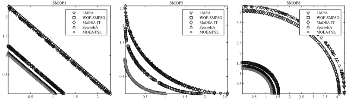
For further observation, Fig. 4 plots the non-dominated solution sets with median IGD values among 30 runs obtained by the five compared MOEAs on SMOP1, SMOP5, and SMOP8 with 10000 decision vari-ables. For SMOP1 with a mostly unimodal landscape, the proposed MOEA/PSL converges better than SparseEA and significantly outperforms LMEA, WOF-SMPSO, and MaOEA-IT. For SMOP8 with complex variable interac-tions, the difference between MOEA/PSL and SparseEA becomes larger. This is because SparseEA does not con-sider any variable interaction when generating offspring

solutions, whereas the proposed MOEA/PSL can learn the variable interactions by RBM and DAE. As for SMOP5 with a unimodal landscape, both MOEA/PSL and SparseEA have satisfactory convergence perfor-mance, since the non-sparse region of the Pareto optimal solutions of SMOP5 is unfixed and quite easy to be de-tected. Moreover, according to the convergence profiles of IGD values obtained by the five MOEAs shown in Fig. 5, it is obvious that MOEA/PSL converges faster than the other MOEAs during the whole evolutionary process. To summarize, the proposed MOEA/PSL can effectively solve sparse LMOPs with various landscapes.

D. Results on Real-World Problems

Table IV shows the HV values obtained by the five compared MOEAs on eight sparse LMOPs in real-world

TABLE IV

HV VALUESOBTAINED BYLMEA, WOF-SMPSO, MAOEA-IT, SPARSEEA,AND THEPROPOSEDMOEA/PSLONFS1–FS3, IS1–IS3, NN1–NN3, CD1–CD3, CN1–CN3, SR1–SR3, PM1–PM3,ANDPO1–PO3, WHERE THEBESTRESULT INEACHROW ISHIGHLIGHTED.

Problem Dec LMEA WOF-SMPSO MaOEA-IT SparseEA MOEA/PSL

FS1 800 2.6893e-1 (0.00e+0)− 8.8087e-1 (5.65e-16)− 2.8697e-1 (0.00e+0)− 9.8467e-1 (4.52e-16)− 9.8478e-1 (3.39e-16) FS2 5966 4.8819e-1 (2.26e-16)− 9.5529e-1 (0.00e+0)− 6.2641e-1 (3.39e-16)− 9.8215e-1 (4.52e-16)− 9.8719e-1 (5.04e-3) FS3 10000 3.3145e-1 (5.65e-17)− 8.9075e-1 (4.52e-16)− 3.7800e-1 (1.13e-16)− 9.7262e-1 (7.90e-16)≈ 9.7443e-1 (7.60e-3) IS1 862 5.9388e-1 (1.38e-2)− 8.7186e-1 (4.59e-3)− 5.7149e-1 (1.85e-2)− 8.4077e-1 (1.07e-2)− 8.9922e-1 (1.78e-2) IS2 4177 4.6320e-1 (1.59e-2)− 7.4703e-1 (3.19e-3)− 4.7467e-1 (7.97e-3)− 7.0593e-1 (9.11e-3)− 8.0424e-1 (2.42e-2) IS3 11055 5.3065e-1 (3.04e-3)− 9.6268e-1 (1.35e-3)≈ 6.7505e-1 (8.71e-3)− 9.5401e-1 (7.10e-4)− 9.6778e-1 (7.31e-3) NN1 1181 3.3298e-1 (1.53e-2)− 4.7043e-1 (1.31e-2)− 3.1841e-1 (9.69e-2)− 9.0530e-1 (1.73e-2)− 9.2951e-1 (3.99e-3) NN2 5161 2.9111e-1 (1.36e-2)− 6.7505e-1 (7.18e-2)− 3.3409e-1 (1.01e-1)− 9.1165e-1 (3.07e-2)− 9.6078e-1 (2.41e-2) NN3 10041 2.6363e-1 (1.49e-2)− 3.4689e-1 (2.69e-2)− 2.6016e-1 (5.04e-2)− 5.8179e-1 (4.53e-2)− 6.6586e-1 (1.48e-2) CD1 1133 9.9357e-2 (2.10e-2)− 6.9976e-1 (1.70e-3)− 3.7719e-1 (8.57e-3)− 5.0006e-1 (0.00e+0)− 7.0540e-1 (1.13e-16) CD2 4039 8.7164e-2 (1.20e-2)− 6.7661e-1 (1.65e-3)− 4.0942e-1 (4.68e-3)− 5.4546e-1 (3.42e-3)− 6.9660e-1 (3.55e-3) CD3 9885 3.1492e-1 (1.28e-3)≈ 5.8850e-1 (2.02e-3)≈ 3.7066e-1 (2.00e-3)− 5.3839e-1 (1.07e-3)− 5.8784e-1 (8.28e-4) CN1 1176 7.0620e-1 (1.77e-2)− 8.6239e-1 (8.82e-3)− 5.9259e-1 (1.40e-2)− 9.4455e-1 (2.72e-3)− 9.7206e-1 (2.12e-3) CN2 4039 5.6216e-1 (3.26e-2)− 7.9818e-1 (9.42e-3)− 5.5264e-1 (1.73e-2)− 8.6601e-1 (1.22e-2)− 9.2460e-1 (5.36e-3) CN3 9885 4.4994e-1 (2.57e-3)− 7.1083e-1 (2.28e-3)− 2.5489e-1 (6.69e-2)− 7.1141e-1 (1.28e-3)− 7.2132e-1 (4.28e-4) SR1 1024 1.5091e-1 (1.23e-2)− 1.1669e-1 (6.35e-3)− 1.0888e-1 (6.59e-3)− 2.6363e-1 (1.62e-2)− 3.2374e-1 (1.91e-2) SR2 5120 1.2704e-1 (7.51e-3)− 9.8539e-2 (2.16e-3)− 9.4736e-2 (2.44e-3)− 2.0594e-1 (6.87e-3)− 2.8826e-1 (6.91e-3) SR3 10240 1.2392e-1 (6.12e-3)− 9.5335e-2 (1.73e-3)− 9.4564e-2 (2.88e-3)− 2.0541e-1 (8.50e-3)− 2.7922e-1 (6.67e-3) PM1 1000 8.2645e-3 (3.53e-18)− 1.0368e-1 (2.01e-3)− 1.4405e-2 (1.08e-2)− 1.5721e-1 (1.71e-3)+ 1.3620e-1 (2.52e-3) PM2 5000 8.2645e-3 (3.53e-18)− 9.4358e-2 (7.33e-4)+ 1.2648e-2 (3.11e-3)− 1.1577e-1 (8.65e-4)+ 8.5430e-2 (1.95e-2) PM3 10000 8.2645e-3 (1.81e-18)− 9.2739e-2 (3.67e-4)− 9.2836e-3 (1.17e-3)− 1.1023e-1 (5.13e-4)+ 9.5855e-2 (3.18e-4) PO1 1000 9.1432e-2 (9.57e-5)− 9.2197e-2 (2.90e-4)− 9.1671e-2 (7.46e-5)− 1.2368e-1 (1.63e-3)≈ 1.2367e-1 (5.84e-4) PO2 5000 9.1120e-2 (2.82e-5)− 9.1244e-2 (5.42e-5)− 9.1120e-2 (1.53e-5)− 1.2380e-1 (1.78e-3)≈ 1.2412e-1 (9.30e-4) PO3 10000 9.1082e-2 (3.97e-5)− 9.1097e-2 (3.77e-5)− 9.1041e-2 (1.06e-5)− 1.2429e-1 (1.48e-3)≈ 1.2481e-1 (2.42e-4)

+/−/≈ 0/23/1 1/21/2 0/24/0 3/17/4

‘+’, ‘−’ and ‘≈’ indicate that the result is significantly better, significantly worse, and statistically similar to that obtained by the proposed MOEA/PSL, respectively.

1e-4 1e-3 1e-2 1e-1

Ratio of selected features 0.01 0.14 0.28 0.42 0.56 Error rate Feature selection 3 LMEA WOF-SMPSO MaOEA-IT SparseEA MOEA/PSL

1e-4 1e-3 1e-2 1e-1 1

Complexity of model 0.35

0.41 0.48

Error rate

Neural network training 3

LMEA WOF-SMPSO MaOEA-IT SparseEA MOEA/PSL

0 3e-6 6e-6 9e-6

Risk 0.96 0.97 0.98 0.99 1 1 - expected return Portfolio optimization 3 LMEA WOF-SMPSO MaOEA-IT SparseEA MOEA/PSL

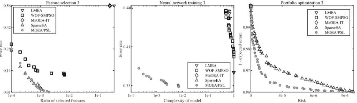
Fig. 6. Non-dominated solution sets with median HV obtained by LMEA, WOF-SMPSO, MaOEA-IT, SparseEA, and the proposed MOEA/PSL on FS3, NN3, and PO3 with approximately 10000 decision variables.

1e5 4e5 7e5 1e6

Number of evaluations 10-1 100 IGD SMOP1 LMEA WOF-SMPSO MaOEA-IT SparseEA MOEA/PSL

1e5 4e5 7e5 1e6

Number of evaluations 100 IGD SMOP8 LMEA WOF-SMPSO MaOEA-IT SparseEA MOEA/PSL

Fig. 5. Convergence profiles of IGD values obtained by LMEA, WOF-SMPSO, MaOEA-IT, SparseEA, and the proposed MOEA/PSL on SMOP1 and SMOP8 with 10000 decision variables.

applications with approximately 1000, 5000 and 10000 decision variables. It can be seen that the proposed MOEA/PSL obtains the best overall performance on

these real-world problems, having achieved the best performance on 19 out of 24 test instances. Besides, SparseEA and WOF-SMOPSO obtain 4 and 1 best re-sult, respectively. Furthermore, Fig. 6 depicts the non-dominated solution sets with median HV values among 30 runs obtained by the five compared MOEAs on FS3, NN3, and PO3 with approximately 10000 decision variables. For the feature selection problem, the solu-tions obtained by MOEA/PSL are slightly better than those obtained by SparseEA and WOF-SMPSO, while LMEA and MaOEA-IT can only find a single solution with bad convergence. For the neural network training problem, the solutions obtained by MOEA/PSL have good convergence and diversity, the solutions obtained by LMEA and WOF-SMPSO are not well-converged, and MaOEA-IT and SparseEA can only find a single

TABLE V

RUNTIMES(INSECOND)OFLMEA, WOF-SMPSO, MAOEA-IT, SPARSEEA,AND THEPROPOSEDMOEA/PSLONBENCHMARK

PROBLEMS ANDREAL-WORLDPROBLEMS.

Problem Dec LMEA WOF-SMPSO MaOEA-IT SparseEA MOEA/PSL SMOP1–

10000 1.1042e+4 5.6467e+3 8.2906e+3 1.0391e+4 6.8868e+3 SMOP8

(average)

FS3 10000 2.4979e+4 2.8925e+3 6.1546e+3 5.4577e+2 4.3347e+2 IS3 11055 2.1538e+5 5.7815e+5 1.3433e+5 4.2568e+4 2.2611e+5 NN3 10041 4.3060e+4 9.3179e+3 4.4536e+3 4.8048e+3 3.5246e+3 CD3 9885 1.2685e+5 4.1383e+4 1.3893e+5 7.5853e+4 6.1153e+4 CN3 9885 5.7187e+4 2.7179e+4 1.2290e+4 3.5482e+4 2.6756e+4 SR3 10240 3.7550e+4 9.2712e+3 7.5098e+3 5.2169e+3 2.6068e+3 PM3 10000 6.4473e+4 9.7101e+4 6.3456e+3 1.5784e+5 1.1052e+5 PO3 10000 8.1801e+3 1.5218e+3 1.9847e+3 2.2545e+3 2.2262e+3

solution. As for the portfolio optimization problem, the solutions obtained by MOEA/PSL have significantly better convergence than those obtained by SparseEA, and the solutions obtained by LMEA, WOF-SMPSO, and MaOEA-IT shrink to the upper-left corner of the objective space. As a consequence, these real-world prob-lems are quite challenging for existing MOEAs, while the proposed MOEA/PSL is more promising for solving these problems than existing MOEAs.

In addition, the runtimes consumed by the five com-pared MOEAs on the eight benchmark problems and eight real-world problems with approximately 10000 de-cision variables are listed in Table V. It can be found that the runtime of MOEA/PSL is not significantly higher than the other MOEAs, though MOEA/PSL should train two neural networks at each generation. This is because the other MOEAs also have complex operations (e.g., variable interaction analysis in LMEA, Pareto-optimal subspace learning in MaOEA-IT, and population ini-tialization in SparseEA), while the neural networks in MOEA/PSL are relatively small and easy to be trained. In short, the proposed MOEA/PSL has competitive effi-ciency to the other MOEAs.

E. Effectiveness of the Two Neural Networks in MOEA/PSL

The proposed MOEA/PSL learns the Pareto optimal subspace by both RBM and DAE, while a single neural network can also be used to achieve this goal. In this case, each solution does not need to be represented by a binary vector and a real vector, and the decision vari-ables can directly be reduced. To verify the effectiveness of using both RBM and DAE, the proposed MOEA/PSL is compared with its variants using a single technique, including random embedding [60], PCA [61], RBM, and DAE. It is worth to note that although there exist many other machine learning techniques able to learn a sub-space, the vectors reduced by most of them are not recoverable, hence they cannot be used in MOEA/PSL.

Table VI lists the IGD values obtained by MOEA/PSL and its four variants on SMOP1–SMOP8 with 1000 de-cision variables. Obviously, the original MOEA/PSL ex-hibits significantly better performance than those with a

single technique on all the test problems. The superiority of using both RBM and DAE is mainly attributed to the consideration of sparsity, where the RBM is used to learn a sparsity distribution and the DAE is used to learn a compact representation. In short, it is necessary to learn the Pareto optimal subspace and consider the sparsity simultaneously in solving sparse LMOPs.

F. Effectiveness of the Parameter Adaptation Strategy in MOEA/PSL

There are two parameters related to the employment of RBM and DAE in MOEA/PSL, i.e., the ratio of off-spring solutions generated in the Pareto optimal

sub-space ρ and the size of the hidden layers K, both of

which are adapted during the evolution of MOEA/PSL. To verify the effectiveness of the parameter adaptation strategy, MOEA/PSL is compared with some of its

vari-ants using a fixedρor K.

Fig. 7 plots the convergence profiles of IGD and HV values obtained by MOEA/PSL with adaptive and fixed

ρ on SMOP7 with 1000 real variables and the instance

selection problem with 862 binary variables. As shown

in the figures, the MOEA/PSL with adaptiveρconverges

faster than the MOEA/PSL with ρ = 0.1, ρ = 0.5, and

ρ= 1. Besides, MOEA/PSL assigns different values toρ

at different generations on different problems. Therefore,

it is unreasonable to set ρto a fixed value; by contrast,

adaptingρduring the evolution of MOEA/PSL can lead

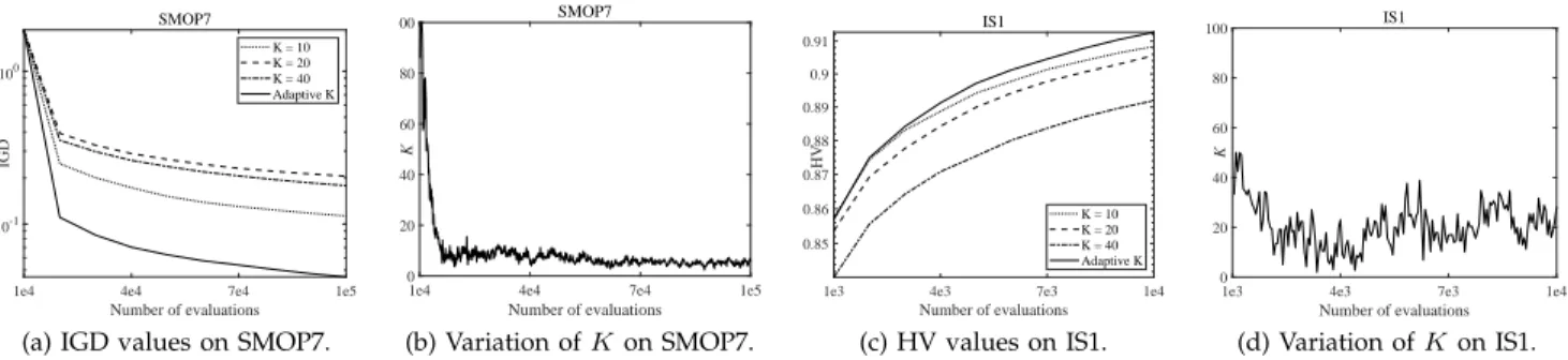
to a relatively good performance on different problems. Fig. 8 plots the convergence profiles of IGD and HV values obtained by MOEA/PSL with adaptive and fixed

K on SMOP7 and the instance selection problem.

Simi-larly, the MOEA/PSL with adaptiveK outperforms the

MOEA/PSL with K = 10, K = 20, and K = 40. To

summarize, the parameter adaptation strategy can not only make MOEA/PSL parameterless, but also improve the performance in solving sparse LMOPs.

V. CONCLUSIONS

To address the limitations of existing MOEAs in solv-ing LMOPs with sparse Pareto optimal solutions, this paper has proposed a Pareto optimal subspace learning based MOEA by using RBM and DAE. In each gen-eration, an RBM is trained to learn a sparse distribu-tion of the decision variables, and a DAE is trained to learn a compact representation. In this way, the decision variables can be reduced by the representation of the hidden layers of RBM and DAE. Moreover, a parameter adaptation strategy has been developed to determine the ratio of offspring solutions generated in the Pareto optimal subspace and the size of the hidden layers.

In the experiments, the proposed MOEA has been compared with four state-of-the-art MOEAs on eight benchmark problems and eight real-world problems taken from various fields. The experimental results have demonstrated that the proposed MOEA is more effective

TABLE VI

IGD VALUESOBTAINED BYMOEA/PSLANDMOEA/PSLWITH ASINGLETECHNIQUE ONSMOP1–SMOP8, WHERE THEBESTRESULT IN EACHROW ISHIGHLIGHTED.

Problem _{(only random embedding)}MOEA/PSL MOEA/PSL_{(only PCA)} MOEA/PSL_{(only RBM)} MOEA/PSL_{(only DAE)} MOEA/PSL SMOP1 9.5389e-2 (5.56e-3)− 3.1069e-1 (5.95e-3)− 1.3810e-1 (1.32e-2)− 3.4657e-1 (8.12e-3)− 1.1507e-2 (2.11e-3) SMOP2 3.6321e-1 (3.41e-2)− 9.5175e-1 (2.24e-2)− 1.5020e-1 (4.21e-2)− 9.7563e-1 (2.62e-2)− 4.2070e-2 (9.70e-3) SMOP3 1.1895e+0 (3.61e-2)− 1.1837e+0 (3.90e-2)− 2.2785e+0 (2.05e-2)− 1.2607e+0 (2.87e-2)− 1.2598e-2 (3.06e-3) SMOP4 6.1402e-2 (1.01e-2)− 4.2656e-1 (1.59e-2)− 5.9898e-2 (6.25e-3)− 4.3297e-1 (1.29e-2)− 4.7175e-3 (2.47e-4) SMOP5 3.9132e-1 (3.36e-3)− 4.0154e-1 (8.31e-4)− 1.2366e-1 (1.77e-2)− 4.1233e-1 (1.30e-3)− 7.4279e-3 (4.60e-4) SMOP6 6.5513e-2 (3.66e-3)− 9.0714e-2 (3.72e-3)− 7.3576e-2 (5.39e-3)− 9.0152e-2 (3.29e-3)− 7.4349e-3 (5.34e-4) SMOP7 2.4670e-1 (2.04e-2)− 2.1980e-1 (1.02e-2)− 3.5022e-1 (6.44e-2)− 2.2567e-1 (5.81e-3)− 5.5240e-2 (3.62e-2) SMOP8 1.1996e+0 (8.21e-2)− 1.2495e+0 (4.09e-2)− 3.7650e-1 (9.77e-3)− 1.2564e+0 (1.95e-2)− 2.2823e-1 (4.59e-2)

+/−/≈ 0/8/0 0/8/0 0/8/0 0/8/0

‘−’ indicates that the result is significantly worse than that obtained by MOEA/PSL.

1e4 4e4 7e4 1e5

Number of evaluations 10-1 100 IGD SMOP7 = 0.1 = 0.5 = 1 Adaptive

(a) IGD values on SMOP7.

1e4 4e4 7e4 1e5 Number of evaluations 0 0.1 0.2 0.3 0.4 0.5 SMOP7 (b) Variation ofρon SMOP7.

1e3 4e3 7e3 1e4

Number of evaluations 0.83 0.84 0.85 0.86 0.87 0.88 0.89 0.9 0.91 HV IS1 = 0.1 = 0.5 = 1 Adaptive (c) HV values on IS1.

1e3 4e3 7e3 1e4 Number of evaluations 0 0.1 0.2 0.3 0.4 0.5 IS1 (d) Variation ofρon IS1. Fig. 7. Convergence profiles of IGD and HV values obtained by MOEA/PSL with adaptive and fixedρon SMOP7 and IS1.

1e4 4e4 7e4 1e5

Number of evaluations 10-1 100 IGD SMOP7 K = 10 K = 20 K = 40 Adaptive K

(a) IGD values on SMOP7.

1e4 4e4 7e4 1e5 Number of evaluations 0 20 40 60 80 100 K SMOP7 (b) Variation ofKon SMOP7.

1e3 4e3 7e3 1e4

Number of evaluations 0.85 0.86 0.87 0.88 0.89 0.9 0.91 HV IS1 K = 10 K = 20 K = 40 Adaptive K (c) HV values on IS1.

1e3 4e3 7e3 1e4

Number of evaluations 0 20 40 60 80 100 K IS1 (d) Variation ofKon IS1. Fig. 8. Convergence profiles of IGD and HV values obtained by MOEA/PSL with adaptive and fixedKon SMOP7 and IS1.

than the compared MOEAs in solving sparse LMOPs with 1000 to 10000 decision variables.

This paper has revealed the necessity of Pareto optimal subspace learning in solving sparse LMOPs. Although the proposed MOEA has successfully achieved this goal by using RBM and DAE, it may become impractical when dealing with sparse problems having millions of decision variables (e.g., deep neural network train-ing [62]), since the population is not large enough for training the neural networks, and the training process will be very time-consuming. Therefore, it is desirable to incorporate the proposed Pareto optimal subspace learning approach into other more effective MOEAs to solve super-large-scale problems.

REFERENCES

[1] J. Liu, M. Gong, Q. Miao, X. Wang, and H. Li, “Structure learning for deep neural networks based on multiobjective optimization,”

IEEE Transactions on Neural Networks and Learning Systems, vol. 29, no. 6, pp. 2450–2463, 2018.

[2] C. Cao, C. Li, Q. Yang, Y. Liu, and T. Qu, “A novel multi-objective programming model of relief distribution for sustainable disaster supply chain in large-scale natural disasters,”Journal of Cleaner Production, vol. 174, pp. 1422–1435, 2018.

[3] S. Mouassa and T. Bouktir, “Multi-objective ant lion optimization algorithm to solve large-scale multi-objective optimal reactive power dispatch problem,”International Journal for Computation and Mathematics in Electrical and Electronic Engineering, vol. 38, no. 1, pp. 304–324, 2019.

[4] L. M. Antonio and C. A. Coello Coello, “Use of cooperative coevolution for solving large scale multiobjective optimization problems,” inProceedings of the 2013 IEEE Congress on Evolutionary Computation, 2013, pp. 2758–2765.

[5] A. W. Iorio and X. Li, “A cooperative coevolutionary multiob-jective algorithm using non-dominated sorting,” inProceedings of the 2004 Genetic and Evolutionary Computation Conference, 2004, pp. 537–548.

[6] K. Deb, A. Pratap, S. Agarwal, and T. Meyarivan, “A fast and eli-tist multi-objective genetic algorithm: NSGA-II,”IEEE Transactions on Evolutionary Computation, vol. 6, no. 2, pp. 182–197, 2002. [7] X. Ma, F. Liu, Y. Qi, X. Wang, L. Li, L. Jiao, M. Yin, and M. Gong,