UCLA
UCLA Electronic Theses and Dissertations
Title
Leveraging Label Information in Representation Learning for Multi-label Text Classication
Permalink https://escholarship.org/uc/item/3870d965 Author Wu, Jiayu Publication Date 2019 Peer reviewed|Thesis/dissertation
UNIVERSITY OF CALIFORNIA Los Angeles
Leveraging Label Information in Representation Learning for Multi-label Text Classification
A thesis submitted in partial satisfaction of the requirements for the degree
Master of Science in Statistics
by
Jiayu Wu
c
Copyright by Jiayu Wu
ABSTRACT OF THE THESIS
Leveraging Label Information in Representation Learning for Multi-label Text Classification
by
Jiayu Wu
Master of Science in Statistics University of California, Los Angeles, 2019
Professor Ying Nian Wu, Chair
The thesis studies the problem of multi-label text classification, and argues that it could benefit from bringing the question into the stage of language understanding. In specific, rather than limit the use of annotated labels to providing supervision in classification only, we also rely on them as auxiliary information to guide the learning of an effective representation that is tangent to the down-stream task. Two approaches are discussed: a) learn a label-word attention layer for composition of label-word embedding into document vectors; b) learn a high-level latent abstraction via an auto-encoder generative model with structured priors conditional on labels. We introduce two designs of label-enhanced representation learning: Label-embedding Attention Model (LEAM) and Conditional Variational Document model (CVDM) with application on real-world datasets, in order to demonstrate their ability in promoting the classification performances with improved interpretability.
The thesis of Jiayu Wu is approved.
Frederic Paik Schoenberg Hongquan Xu
Ying Nian Wu, Committee Chair
University of California, Los Angeles 2019
TABLE OF CONTENTS
1 Introduction . . . 1
1.1 Motivation and Challenges . . . 1
1.2 Outline and Contributions . . . 2
2 Preliminaries . . . 4
2.1 Task Statement . . . 4
2.2 Representation Learning . . . 4
2.2.1 Word representation . . . 5
2.2.2 Document representation . . . 7
2.2.3 Latent Variable Inference . . . 8
2.3 Multi-label Classification . . . 10
3 Methodology . . . 12
3.1 Leveraging Label Information . . . 12
3.2 Multi-label LEAM Model . . . 14
3.3 Conditional Variational Document Model . . . 15
4 Experiments . . . 18
4.1 Experiment setting . . . 18
4.2 Evaluation metric . . . 20
4.3 LEAM Results and Analysis . . . 21
4.4 CVDM Results and Analysis . . . 25
6 Appendix . . . 30
LIST OF FIGURES
3.1 Illustration of the use of label information . . . 12
4.1 Reuters Performance over Training Epoches . . . 21
4.2 anon-Rev Performance over Training Epoches . . . 21
4.3 Reuters label correlation heatmap (subset of 50) . . . 24
LIST OF TABLES
4.1 Data Description . . . 18
4.2 LEAM Results Comparison . . . 21
4.3 Reuters Highlight Samples . . . 23
4.4 Ablative Analysis on Reuters . . . 24
4.5 General Comparison of Results . . . 26
4.6 Comparison between generative models . . . 26
4.7 Top-words for some topics . . . 27
6.1 Reuters Results . . . 31
6.2 anon-Rev Results . . . 31
CHAPTER 1
Introduction
1.1
Motivation and Challenges
Multi-label classification is a common task in natural language processing (NLP). It assigns the most relevant label(s) to a given text document, and is widely applied for review catego-rization, tag recommendation, information retrieval, etc. The rapid growth in modern data scale is making it increasingly important as well as challenging.
Conventionally, text data can be processed with manually designed label taxonomy and naive labeling methods like regular expression matching. It is obviously not accurate nor efficient enough, and fails to achieve a generalizable understanding of the language.
Going beyond keyword matching, most statistical models and machine learning tech-niques favor well-defined, fix-length inputs, while the representation of textual data is non-trivial in NLP. Word entities are discrete in form while rich in connotation, and the serial correlation in natural utterances also makes feature extraction more difficult.
In addition, multi-label classification can be harder than the single-label multi-class prob-lem, due to the huge solution space and the potential label structure. Traditional machine learning techniques like binary relavence and label powerset suffers from a high computa-tional cost and unbalanced label distributions. Meanwhile, deep learning methods usually require considerable annotated training samples as well as high computational power, and the model tend to be domain-specific and hard to interpret.
This thesis attempts to look into these challenges, and argues that using label information as auxiliary knowledge in the learning of text representation can facilitate the down-stream classification task and increase model interpretability. Intuitively, instead of assigning labels
after finishing the reading, we make the algorithm ’aware of’ the task and the possible labels to choose from even before it looks at the text. In this way, the representation of the messy textual data is not only aided by contextual information, but also more tangent to the classification task.
We introduce two approaches to this end: a) learn a label-attention layer after the word embedding layer, and b) learn a latent semantic vector for each document via generative model.
1.2
Outline and Contributions
This thesis is organized in five parts. In the first chapter, we introduce the multi-label text classification task with its main challenges, and state the purpose of this thesis. In Chapter 2, we formally define the task, and review previous literature on the learning of text representation and the training of multi-label classification models respectively, with specific interests in recent advances by using auxiliary knowledge in representation learn-ing. The methodology will then be detailed in the next chapter. We discuss two models: Lable-Embedding Attention Model (LEAM) and Conditional Variational Document Model (CVDM). In Chapter 4, we assess both models on real-world datasets to demonstrate how the classification is boosted and made more interpretable with the use of label-enhanced repre-sentation, and some abalative analysis is also presented. Finally, conclusion and discussions will be presented.
The contributions of our work are as follows:
1. argue that using labels information in the stage of text representation learning can facilitate the multi-label classification tasks with improved model interpretability;
2. introduce two sorts of label-enhanced representation learning methods and construct the models for multi-label classification:
• LEAM: multi-label extension of the multi-class LEAM [42] that introduces atten-tion mechanism between word and label embedded in the same space
• CVDM: latent variable model under the neural variational inference framework with latent prior conditioned on labels.
3. demonstrate that LEAM significantly improves multi-label classification performances, and the decision is made more interpretable due to the learnt attention weights, and scales well to a large number of labels and unbalanced samples.
4. show that CVDM achieves classification performance comparable to benchmark gen-erative methods as well as discriminative classification methods, with a more flexible and generalizable neural network structure.
CHAPTER 2
Preliminaries
2.1
Task Statement
Consider a corpus withN documents. Each documentdis a sequence{w1,w2, ...,wi, ...,wm}
where w’s are word tokens, and m is the length of the document. In order to extract numerical features from it, we denote the p-dimensional vector representing a word tokenw
as x, and the vector representation of a document Xd.
Since each document dis associated with an indefinite number of labels, we represent the label with a binary vector Yd =
y1,y2, ...,yl, ...,yL|,yl ∈ {0,1} where L is the number of potential labels in total. We drop the subscript d for simplicity, thus the objective is to predict a set of most relevant labels Y for a document d represented byX.
The task could be decomposed into two phases in modeling: design or learn a quanti-tative representation of the text documents, and perform multi-label classification on that representation. We are especially interested in the mapping of a sequence of word entities to a fixed length document vector or a latent variable Z with the help of the annotated labels:
X =f(x1,x2, ...,xi, ...,xm;Y) and/or Z =f(X;Y).
2.2
Representation Learning
The representation of textual data is a prevalent challenge in modeling language. Natural utterances are sequences of discrete entities of indefinite lengths, while the semantic nuances as well as the syntactic rules entailed are hard for even human learners to command. In contrast, most modeling and learning algorithms prefer well-defined, fixed-length numerical
data and tend to be limited to differentiable functions. Therefore, an important problem in language processing is to extract from the textual data numerical features capable of representing various linguistic properties of the text [11].
2.2.1 Word representation
”Without grammar, very little can be conveyed; without vocabulary, nothing can be con-veyed” [46] . Word tokens are commonly used as the lowest level modeling components in NLP as the basic abstract units of meaning. Representing a word is the design or learning of a mathematical object associated with each word, often a vector [40].
Discrete symbols
Regarding word tokens as discrete symbols, a generic way is to represent each word by a one-hot vector, the vector dimension is then the size of the vocabulary denoted as |V|. With a high volume of vocabulary, such representation is extremely sparse as well as high-dimensional, and lacks a similarity measure between words.
To capture the relationship between words, graphically structured dictionary (taxonomy) that links synonym and hypernym together are designed, an example is the word-net [23]. However, it requires massive human expertise and labor, as the constant development of language is making an accurate and up-to-date dictionary hard to maintain. Nevertheless, the similarity is still hard to quantify objectively.
Word embedding
In recent years, the pursuit of word embedding has become popular, especially deep neural network models motivated by the development in computation power and the success of pre-trained feature extractors in the field of computer vision. Empirical evidences have shown that the effectiveness of word embedding can be the key to improvement on various NLP task, including and not limited to text classification [3][26].
Word embedding is real-valued, fixed-length dense feature vector of the word, of which the dimension is usually far more compact than the vocabulary size. It is also called distributed representation [3][40], because it is usually learned unsupervised with the assumption known
as distributional hypothesis [1][12], that is, similar words should have similar contexts. The learnt representation not only is reduced in dimension, but also provides a simple word similarity measure by distance or angle (ex. cosine similarity) between vectors. Hopefully, each embedding dimension represents a meaningful latent syntactic or semantic feature of the word [40], which even makes word analogy possible, such as man:woman ∼ king:queen.
In general, word embedding can be learnt from global or local co-occurence information. The former is by factorization or low-rank approximation on a global relational matrix from a general corpus. An example is Latent Semantic Analysis (LSA) [8] that applies SVD to a term-document matrix. The later is to build a predictive model for the local context of each word, where neural language models (NNLM) are prevalent. NNLM solve for a language model that is capable of predicting the most probable word given its context, and the vector representation (usually the first hidden layer) corresponding to each word can be output as word embedding x.
Many efforts have been made towards higher efficiency and performance since the first large NNLM proposed by Bengio in 2003 [3]. Word2Vector introduces two popular frame-works, Skip-Gram and Continuous Bag-of-Words, which can be seen as a two-layer network with an efficient architecture providing nice semantic properties [22]. Interestingly, there is also a proven connection to the global embedding methods, as it implicitly factorizes globally shifted word-context matrices with pair-wise information measures [18]. Another prominent word embedding architecture, GloVe [26], leverages both the local context window and the global co-occurrence matrix via a bilinear regression model. ELMO further model the different usage of the same word by learning multiple levels of syntactic and semantic information about words in-context [27]. A most recent advance in 2018, BERT, achieves state-of-the-art performances on a vast of tasks via a transformer neural architecture and two novel objectives: predict masked words and next sentences [9].
Word embedding is significant as a pre-train method widely used in NLP, which makes learning transferable between various text domains and tasks. The embedded features can be used directly for down-stream task, or fine-tuned over specific tasks [9][29]. It is notable that, both the application of word embedding and the training of language models require the
composition of the representations of single words into that of the training units - sentences or documents.
2.2.2 Document representation Bag-of-words
A simple way to represent document is to add up all one-hot word vectors, resulting in a document vector that is an occurrence count of the vocabulary. It is called bag-of-words (BoW), because only content is preserved and the order information discarded. It can be generalized to n-gram model which counts all unique contiguous sequences of n tokens instead of single words, such that some multi-word expressions can be identified.
Although BoW does not tap into the word-level nuances, it is still a simple and useful feature extractor for documents. Intuitively, similar documents tend to have similar distri-butions over the tokens, and occurrence of certain words can be indicative of the document semantic. Representing the word distribution by count, however, can be biased by the vary-ing lengths of documents and certain words frequent in the whole corpus (ex. ’the’, ’is’). Therefore, Term Frequency Inverse Document Frequency (TFIDF) is motivated, which uses the frequency normalized by length and rescaled by how often they appear in the whole corpus to penalize words that dominate. The resulting value corresponding to each word indicates how informative the word is in distinguishing this document from the others.
Neural networks and attention
As for the composition of word embedding, there are studies showing that simply averag-ing [45] or max-poolaverag-ing [31] achieves excellent performance given a good enough embeddaverag-ing. Nonetheless, there are also more sophisticated methods attempting to incorporate structural or temporal correlation. Neural networks, as powerful approximator for complex nonlinear functions, are popular choices for not only learning of language models but also down-stream NLP tasks.
The local context and serial correlation between words motivates the prevalent use of convolutional networks (CNN) and recurrent networks (RNN) [27][53]. Long-short Term
Memory (LSTM), a variant of RNN, stands out due to its ability to reduce the gradient vanishing of signal faraway, which improves the performances over longer sentences. Bi-direction LSTM benefits from the context after the word as well as that comes before it, by concatenating two feature vectors learnt on both direction. It achieves excellent performances in language model architectures like ELMO as well as in various NLP tasks [48][50]. However, RNN has the drawback that the sequential computation cannot be parallelized, hence takes longer time to train.
Attention mechanism is an important technique to promote the efficiency in modeling distant dependency, while maintaining a simple, interpretable and parallelizable structure. Attention models dynamically ’pay attention to’ (put more weight on) certain parts of the input that is more relevant to the task at hand than others, and can be flexibly incorporated to different levels of representation or threads of inputs [6]. Not only can it incorporates other structures like RNNs [2], Transformer architecture bypasses the inefficient RNNs by modeling sequences purely based on a stack of multi-head self-attention over position embedding and content embedding [41].
In text classification tasks, attention models are mainly used for better document repre-sentation. An example is HAN proposed by Yang et al. that achieves a SOTA performance with both word-level and sentence-level attention [49].
2.2.3 Latent Variable Inference
Another way to extract a compact representation of messy raw data is via latent variable in-ference or generative statistical models [25], which is useful not only for signal generation like in machine translation or question answering, but also for obtaining efficient and hopefully interpretable latent representations.
Latent variable models assumes that there exists a hidden variable underlying the ob-served data X, denoted as Z. It can be considered as the hidden structure from which the observed data are generated, or as a high-level abstraction of the data. Thus the marginal data probability can be defined via Bayes rule: p(X) = R p(Z,X)dZ. By introducing an
approximatorq(Z), the evidence lower bound (ELBO) can be derived by Jensen’s Inequality (see appendix):
logp(X)≥ELBO =Eq[logp(X,Z)]−Eq[logq(Z)] =Eq[logp(X)]−DKL(q(Z)kp(Z|X))
EM algorithm can be used to iteratively update q(Z) when the posterior distribution is in a known form. However, the posterior is intractable in most cases, then Monte Carlo sampling or Variational Bayes may be sought for approximation.
In language processing, topic models are widely explored, which explains text by a spec-ified number of unobserved classes [5][13]. It considers document with BoW encoding, and assumes a probabilistic generative process that each document corresponds to a topic sam-pled from a corpus-specific multinomial distribution over all potential topics, then each word in that document is sampled from a topic-specific multinomial distribution over the whole vocabulary:
yl∼Multinomial (θθθ), θθθ∼p(α0)
wi ∼Multinomial (βl)
Hereyl is the discrete latent variable indicating thel-th topic,θθθ is a corpus-level param-eter sampled from the a prior distribution with hyperparamparam-eter α0, and βl parameterizes
the word distribution corresponding to the topic yl. It can also be generalized to document models, where latent semantics are assumed represented by a continuous vectors instead of discrete topic.
A successful model, Latent Dirichlet allocation (LDA) relies on the conjugate prior, Dirichlet distribution θθθ ∼ Dirichlet(α0), α0 ≥ 0, for analytical computation to the
poste-rior over the discrete latent topics [5]. There are also extensions to incorporate annotated labels and even multi-label information, like in semi-supervised LDA or Multi-label Topic Model [33]. All these methods require certain assumption for approximation and meticulous derivation for tractable computation.
Whereas, more expressive models are in increasing demand to accommodate more com-plex and diverse problem with different sources of information, where closed-form derivation are often non-trivial and hard to generalize. Variational auto-encoder (VAE) introduced
the idea to learn a approximate posterior probability q(Z|X) parameterized by an neural inference network, rather than rely on analytic approximation as in traditional variational Bayes [16]. They propose a different variational lower bound that matches the approximate posterior to a prior (see Appendix):
logp(X)≥ LV AE =Eq(Z|X)[logp(X|Z)]]−DKL(q(Z|X)kp(Z))
q(Z|X) and p(Z) are usually assumed to follow distributions easy to sample from, such as gaussian or uniform distribution, thus it is capable of learning complicated non-linear distributions with strong generalisation ability as well as simple computation.
The success of VAE motivates a vast of extensions under the Neural Variational Infer-ence framework, for signal generation as well as latent variable inferInfer-ence [37]. Miao et al. proposed several neural topic and document models (NVDM, NVTM), where the inference is conditioned on easy samples from multivariate gaussian, and the model architectures are designed to discretize the variable while preserving some conjugacy property [20][21]. How-ever, a drawback to these models is that they are fully unsupervised, so the learning can not make full use of the known context, and the learnt latent topics are not always coherent.
2.3
Multi-label Classification
Assigning multiple labels is natural for many real scenarios including text processing, as each document usually belongs to more than one semantic categories. It is a more challenging than single-label problem, as the solution space grows exponentially with the the size of the labelsLand the distribution of available samples over the labels can be very unbalanced. For example, among the 90 labels in the benchmark dataset Reuters, some labels have thousands of training sample, whereas the least populated label is seen only once in the training.
The related models can be categorized into two types: problem transformation methods, and algorithm adaptation methods [38].
The former transform the multi-label task into single-label classification or regression problems, and choose corresponding algorithm to solve it. A common example is the Binary
Relevance (BR), also referred to as one-vs-all, which independently train one binary classifier per label to tell apart it against all the others. To further consider the label correlations, there are label powerset (LP) that train a multi-class classifier on all unique label combinations [39], and classifier chains (CC) that train a chain of binary classifiers [30]. They are mostly strong baselines with simple intuition and implementation, however, the computational cost usually scales with the label size.
Algorithm adaptation methods extend specific learning algorithms to handle multi-label data directly. Ensemble tree methods are widely explored, Clare and King extend entropy to multi-label scenario [7], and FastXML improves the accuracy by learning a hyperplane to split instances rather than selecting a feature subset at each node [28]. Ranking-based methods are also popular choices, such as Rank-SVM [10], ML-KNN [52]. They are more computationally efficient than most problem transformation methods, yet the selection of a decision threshold is usually required.
BP-MLL was one of the first to use neural network for multi-label tasks by a pairwise ranking loss [51]. More recent research, however, reported that binary cross entropy loss with rectified linear units (ReLU) outperforms the pairwise ranking loss with higher efficiency [24]. Such feed-forward architectures are easy to execute, yet they relied on the parameter itself to exploit the dependency across labels.
More sophisticated architectures are proposed in many recent works. Wei et al. pro-posed a modified architecture for multi-label image classification [44]. SGM use RNN to sequentially generate label predictions in order to learn label correlation, and using label co-occurrence statistic in network initialization is also proven to better capture label depen-dencies [17]. Label embedding methods are greatly improves the efficient when the label space is huge and sparse, which compress the labelY to a low dimensional latent space, and decompress the predicted embedding to the original label space [4].
CHAPTER 3
Methodology
3.1
Leveraging Label Information
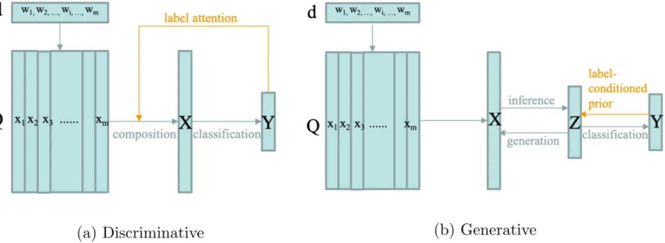
We introduce two approaches to leverage the annotated labels Y in the representation of textual data, in the scenarios of discriminative learning and generative learning respectively. As illustrated in Figure 3.1, the former enhance the document representation by introducing attention between label-word pairs, and the later imposes structure in latent representation by matching the posterior to label-conditioned priors. Both are capable of producing repre-sentation of the original document that are more tangent to the down-stream classification task.
(a) Discriminative (b) Generative
Figure 3.1: Illustration of the use of label information
Label attention
As mentioned before, several text classification models use the attention mechanism for a good representation of the text sequence [19][49]. Nevertheless, these model mainly focus
on self-attention that applies attention to each word-word pair from the text itself, while auxiliary information are less explored even though the attention between words and labels is directly related to the target task.
Label-Embedding Attentive Model (LEAM) is a recent state-of-the-art text classification model proposed by Wang et al.[42]. It embeds words and labels to the same latent space, and aggregates the word embedding into the document representation attended by the label embedding. Moreover, the prediction is made more interpretable by outputting the attention weights for each word as a by-product, which may also provide informational anchors for human speed reading and assessment.
Despite the novel idea and excellent results, the original work did not analyze the effect of the pre-trained embedding and attention structures in the architecture. We will detail the model in Section 3.2, and implement it for experiments on real-world multi-label tasks and further compare some ablative methods.
Conditional VAE
The vanilla VAE framework has the drawback that its inference process is fully unsuper-vised without leveraging auxiliary knowledge. It not only limits its interpretability, but also reduces the inference ability. Namely, the inference network either matches all the latent representations closely together to the one priorp(Z), though they can be multi-modal in na-ture (ex. from different classes), or fail to learn an effective inference because the generative objective dominates the objective function [54]. Many research have contributed to improv-ing the quality of autoencoder-based representation learnimprov-ing [36][37], either by modifyimprov-ing objective function [54] or imposing structured prior [14].
Conditional VAE (CVAE), is motivated by the need to generate more diverse signals (images or answers) conditioned on certain context attributes [32][47][55]. It defines a prior network to learn the prior distribution conditional on known attributes (ex. classes), and the variational lower bound conditional on the attributes can be rewritten in accordance (see Appendix) [34]. CVAE is also applied on the task of zero-shot image classification, to aid the prediction of unseen classes by sharing prior network between the seen classes with the
unseen ones [43].
We intend to incorporate the idea into NVDM to build a supervised generative model for text categorization. The proposed model will be described in Section 3.3 and compare with traditional supervised LDA in the experiments.
3.2
Multi-label LEAM Model
We denote the embedding of a wordwase-dimensional vectorx, and construct a embedding matrix concatenating all the words in the whole document as: Q = {x1, ...,xi, ...,xm} ∈ R(e×m). We also embed the labels Y into the same embedding space, denoted as C =
{c1, ...,cl, ...,cL} ∈R(e×L). Then we align all the label-word pairs via the cosine similarity:
G= C |Q
|C| · |Q| (3.1)
G ∈R(L×m) measures the similarity between each label and word token with respect to the document, in order to determine how relevant a word is to each label. Nonetheless, the local context can impact the word meaning, so an 1−d convolution with ReLU activation is added on to obtain an alignment between the label and each 2r+ 1 gram window center at word wi:
a={a1, ..., ai, ..., am} ai =ReLU(Gi−r:i+rW +b) (3.2)
Then the attentionαααis obtained by max-pooling and softmax, resulting in the weights for each word in the document, and finally the composition of the document vector is computed as the weighted average:
ααα ={α1, ..., αi, ..., αm} αi = softmax (max-pooling (ai)) (3.3) X= m X i αixi (3.4)
The label-attended document representation Xcan be used as the input to a multi-label classification algorithm, the embedding weights and attention parameters can be learnt or fine-tuned simultaneously with the classifier. In our experiments, we compare on different
datasets the effect of using a pre-trained word embedding and learn the embedding from random initialization in the target corpus.
An interesting byproduct of LEAM, is the attention weights on each wordααα, such that we may highlight the most ’important’ (more weights in the representation composition) words in the document. It will also be exemplified in the experiments. In addition, there are several potential variants of LEAM architecture. The word-label alignment can be computed in alternative ways. Some of them will be compared in the experiments.
3.3
Conditional Variational Document Model
We propose Conditional Variational Document Model (CVDM) by introducing class-conditioned priors into NVDM by Mian et al. [20], and use a KL-divergence based ranking score for clas-sification prediction similar to VZSL by Wang et al.[43].
We denote the BoW encoded document as X, and assume there exists a high-level se-mantic abstraction notated by a p-dimensional latent variable Z. The posterior distribution
p(Z|X) is approximated by a isotropic Gaussian distribution parameterized by an inference network f(·;φ):
qφ(Z|X)∼N(fµ(X;φ), fσ2(X;φ)Ip) (3.5)
In order to leverage the label information, we assume the prior distribution of latent vari-ableZis conditional on the label setY, and the distribution parameters are learnt by a prior network gµ(·;ψ), which can be a multi-layer perceptron or a simple linear transformation:
p(Z|Y,A) = L Y l p(Z|yl)y l = L Y l N(gµ(al;ψ), gσ2(a l;ψ)I p) yl (3.6)
Here A = a1, ...,al, ...,aL are the attributes associated with each label, they can be learnt from random initialization or use additional features, for example, features extracted by TF-IDF over all the documents associated with each label.
For better interpretability, we assume each document is generated over a mixture of labels following a similar intuition to topic models. In specific, each label defines a multinomial
distribution over the vocabulary parameterized byβl, and the occurrence of each label follows
a Bernoulli distribution parameterized byθθθ that is conditioned on samples from the latent variable ˆZ: yl∼Bernoulli (θl), θθθ = sigmoid( ˆZU) = [θ1, ..., θl, ..., θL] w∼Multinomial(βl), β = softmax(V) = [β1, ..., βl, ..., βL] (3.7)
where U ∈ R(p×L), V ∈R(L×|V|) are learnable weight parameters. Therefore, by sampling ˜Z
from the posterior and compute topic distribution parameter ˜θθθ˜˜, the label indicatorylcan be
integrated out as:
logp(X; ˜θθθ, β˜˜ ) = m X i h logp(wi; ˜θθθ, β˜˜ ) i = m X i " log L X l h p(wi;βl)p(yl; ˜θl) i # = log(˜θθθ˜˜·β) (3.8)
We may derive the variational lower bound as follows:
logp(X|Y,A)≥Eq(Z|X;φ)[logp(X;θθθ, β)]−DKL(q(Z|X;φ)kp(Z|Y,A;ψ)) =Eq(Z|X;φ)[logp(X;θθθ, β)]−Eq(Z|X;φ)[logq(Z|X;φ)] + L X l yl·Eq(Z|X;φ) logp(Z|al;ψ) =Eq(Z|X;φ)[logp(X;θθθ, β)]− L X l yl·DKL(q(Z|X;φ)kp(Z|al;ψ)) +const.
Since the last term is an additive constant, we may formulate the CVAE Likelihood as:
LCV AE = 1 N N X d " log(X;θθθ;θ, β)− L X l yld·DKL(q(Zd|Xd;φ)kp(Zd|ald;ψ)) # (3.9)
A trivial solution to maximize LCV AE, however, is to learn the same prior distribution p(Z|yl;ψ) for each label, which reduces the model to the original VAE with a standard gaussian prior. Therefore, we augment the objective with a margin regularizer. We encourage
q(Z|X;φ) to be far away from irrelevant labels by penalizing the maximum-margin between the next best label. Since the hard maximum is non-differentiable, we use the smooth surrogate log-sum-exponential trick:
LREG= log L X l (1−yl)·exp−DKL(q(z|X;φ)kp(zd|ald;ψ)) (3.10)
The final objective function to be optimized is: L = N1 PN d{logp(Xd;θ, β)− PL l y l d·DKL(q(Zd|Xd;φ)kp(Zd|ald;ψ)) −λ·logPL l(1−y l)·exp −DKL(q(z|X;φ)kp(zd|ald;ψ)) } (3.11)
Given the trained model parameters, the prediction on a testing document X from that corpus can be obtained by first encoding the feature X into variable Z, and sample a latent variable or use the mean as ˆZ, then selecting the most probable labels. The generative learning process has provided a natural choice of scoring: KL-divergence measuring the distance between the latent variable to the label-conditioned priors:
ˆ
yl=1[sigmoid(−DKL(q(Z|X;φ)kp(Z|al;ψ))) > T] (3.12)
Here T is a decision threshold. Since the KL-divergence term is greater than 0, the resulting score is always less than.5, so we selectT empirically by grid-search on the interval (0,0.5] to find a T with minimum macro-F1 score.
CHAPTER 4
Experiments
4.1
Experiment setting
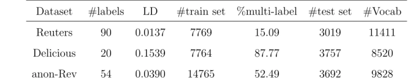
We evaluate LEAM and CVDM empirically on three English text datasets: Reuters, De-licious and anon-Rev. The first two are public annotated datasets, and the last one is an anonymous business review datasets provided by Stratifyd Inc. The data attributes are listed in Table 4.1. Here we define Label Density (LD) as the average number of labels per sample divided by the size of labels, in order to quantify to which a dataset is multi-label:
LD= N1 PN
d=1 |Yd|
|L| .
Dataset #labels LD #train set %multi-label #test set #Vocab Reuters 90 0.0137 7769 15.09 3019 11411 Delicious 20 0.1539 7764 87.77 3757 8520 anon-Rev 54 0.0390 14765 52.49 3692 9828
Table 4.1: Data Description
The Reuters is a benchmark financial newswire dataset for document classification, and we use its ”ApteMod” subeset1, and keep only the alphabetic vocabulary appear at least
three times. The Delicious dataset2 [56] contains tagged web pages retrieved from the social bookmarking site delicious.com with 20 common tags, we adopted the preprocessed and partitioned version by Soleimani and Miller3 [33]. The anon-Rev dataset contains online
1http://kdd.ics.uci.edu/databases/reuters21578/reuters21578.html
2http://nlp.uned.es/social-tagging/delicioust140/
reviews on banking services, labeled by the keyword matching method. In all experiments, we split the training data into train and validation by a ratio of 4:1 for threshold selection and tuning purpose.
For the Delicious dataset, we use the same preprocessing procedure by Soleimani and Miller [33] for a fair comparison with their experiment results in section 4.4. This version uses a larger stopword set, and performs word stemming in order to obtain a more compact BoW representation. As a result, GloVe embedding is of little use and some sequential info can be lost, so we will focus on CVDM for this dataset.
In LEAM implementation, we employ 300 dimensional word embedding and set the convolution window size as 8, a maximum length ofm= 100 is fixed for each document. We train a two-layer MLP with 256 hidden units and binary cross entropy loss as the multi-label classifier. In *LEAM, we learn the embedding weights from random initialization. In the pre-trained version (GloVe-LEAM), we use 300−dGloVe embedding pre-trained on Wikipedia 2014 + Gigaword 5 as embeddings weights initialization, and the Out-Of-Vocabulary (OOV) words are initialized from a mean embedding over the whole vocabulary.
As for CVDM, we set the inference network to be a two-layer MLP with 256 hidden units each, and the latent variable dimension is set to p= 60. The prior net uses a simple linear transformation, and in *CVDM, we learn a 128-dimension label attributes A from random initialization while the TFIDF-CVDM uses 128-dimension TF-IDF features. The regularization parameterλis set to 1, and in each epoch we alternatively update the encoder and the decoder.
We compare our models with two strong baselines based on neural network methods, BoW-MLP and GloVe-MLP. The former takes BoW encoded documents as input, while the later learns embedding weights from GloVe initialization and the document vector is built by mean-pooling over word vectors. Both train two-layer MLP as classifiers.
We use Adam Optimizer [15] with an initial learning rate of 0.001 and a minibatch size of 128, dropout regularization is employed on each hidden layer with a 0.5 rate. The performances are evaluated on the testing set unseen in training if not specified otherwise.
4.2
Evaluation metric
The evaluation for multi-label classification should be different than those for single-label targets, since the prediction for each example can be partially right as well as being com-pletely right or miss. We introduce several metrics to assess and compare the performance in our experiments. The true label set is notated as binary vector Y, and similarily the predicted as ˆY.
If we consider only the complete right cases as accurate prediction, we have a simple and strict measure Exact Match Ratio [35] :EM R= N1 PN
d=11(Yd= ˆYd).
In order to account for partial correctness, Godbole et al. adopted Hamming Scoreto measureMultilable Accuracyas a symmetric measure of the distance between two binary vectors: Accuracy = 1 N N X d=1 |Yd∩Yˆd| |Yd∪Yˆd|
and corresponding Precision, Recall and F1measures:
P recision= 1 N N X d=1 |Yd∩Yˆd| |Yˆd| Recall = 1 N N X d=1 |Yd∩Yˆd| |Yd| F1 = 1 N N X d=1 2|Yd∩Yˆd| |Yd|+|Yˆd|
These are also called Micromeasures, where True Positive (TP) and False Positive (FP) are counted globally and averaged per sample. Because they care more about positives then negatives, more frequent labels may dominate the measure. To alleviate that, we also have
Macromeasures, where statistics are computed for and averaged over each classes such that they are given the same weight:
macro−F1 = 1 L L X l=1 2|Yl∩Yˆl| |Yl|+|Yˆl|
As mentioned before, thresholding can affect the classification accuracy, especially for ranking-based algorithms. Therefore, to assess and compare the ranking performance, ROC-AUC can be used, which is the area under the receiver operating characteristic. Similarly, it also has Micro and Macro measures [33].
4.3
LEAM Results and Analysis
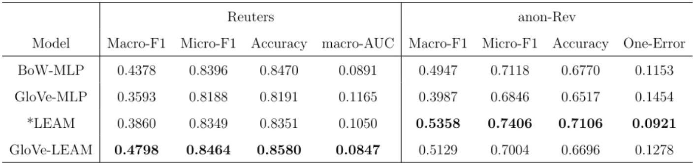
Table 4.2 compares the LEAM results on Reuters and anon-Rev. The performances over training processes are plotted in Figure 4.1 and Figure 4.2 respectively, in which the middle one display the testing macro-F1, the left one shows the micro-F1 and the right one training macro-F1. It can be observed that micro-F1 hardly tells apart different models, while macro measure is less biased by high-frequency labels.
Reuters anon-Rev
Model Macro-F1 Micro-F1 Accuracy macro-AUC Macro-F1 Micro-F1 Accuracy One-Error BoW-MLP 0.4378 0.8396 0.8470 0.0891 0.4947 0.7118 0.6770 0.1153 GloVe-MLP 0.3593 0.8188 0.8191 0.1165 0.3987 0.6846 0.6517 0.1454 *LEAM 0.3860 0.8349 0.8351 0.1050 0.5358 0.7406 0.7106 0.0921 GloVe-LEAM 0.4798 0.8464 0.8580 0.0847 0.5129 0.7004 0.6696 0.1278
Table 4.2: LEAM Results Comparison
Figure 4.1: Reuters Performance over Training Epoches
Figure 4.2: anon-Rev Performance over Training Epoches
On Reuters, the pre-trained GloVe initialization greatly improves Macro-F1 that indi-cates better predictions on rare classes, and is less prone to overfit. As for anon-Rev, *LEAM is slightly better. We hypothesize that it is related to the difference in vocabulary domain. GloVe is trained on newswire stories and encyclopedia, and is closer to the domain of Reuters collection. Whereas, non-Rev tend to use informal language with a relative smaller vocabu-lary, and the label distribution is more balanced, hence the word embedding can be learnt more effectively within the corpus.
In Figure 4.1 it can be observed that GloVe-LEAM achieves the best testing macro-F1 by a large margin, while the training performance and the micro measure of the strong baseline BoW-MLP is almost as good if not better, which demonstrates that LEAM is less prone to overfit or influenced by the unbalanced label distribution, even when the data sparsely populates on a large number of labels in Reuters.
Compared to GloVe-MLP, GloVe-LEAM is only different in the one-layer label embedding and the one-layer attention, however the improvement in performance is substantial. A good word embedding itself does not suffice and the convergence can be very slow even though our network is shallow, which further illustrates that the label attention mechanism effectively promotes the representation of sequence with a simple and interpretable structure.
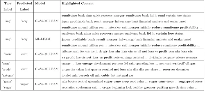
Table 4.3 shows some samples where the word is in a bold font if the learnt attention weights is greater than 0.015 (among 100 in length). Keywords indicative of the label is marked, even if they do not share the same etymology with label words. For example, ’crop’ is identified for label ’grain’, ’merge’ and ’profitable’ for label ’acq’, while some phrases are less stressed such as time, places and prevalent transitions of ’someone said’. Comparison between GloVe-LEAM and *LEAM on the same text (Line 1 and 2) indicates that the pre-trained embedding facilitates the learning of more spiky attention weights, while *LEAM is slightly inferior in distinguishing irrelevant words like ’osaka’ or ’japan’, probably because the learnt embedding is not sufficient in capturing the distance between entities such that the label-word alignments are harder to learn.
example, ’net loss’ is frequently recognized for the label ’earn’, likely due to the use of convolution over label-word alignment. Interestingly, the prediction also seems to capture some correlation between labels, for example, ’crude’ and ’oil-gas’ are predicted together when the text is lack of evidence for ’crude’.
Ture Predicted Model Highlighted Content Label Label
’acq’ ’acq’ GloVe-MLLEAM
sumitomobank aims quick recoverymerger sumitomobank ltd ltsumicertain lose status japanprofitablebank resultmerger heiwasogo bank financial analysts said osaka based
sumitomoaround trillion yen ... interview saidmergerinitiallyreduce sumitomo profitability...
’acq’ ’acq’ ML-LEAM
sumitomo bankaimsquickrecoverymerger sumitomo bankltd lt certain losestatus
japan profitable bank result merger heiwasogo bank financial analysts saidosakabased
sumitomoaround trillion yen ... interview saidmergerinitiallyreducesumitomoprofitability...
’earn’ ’earn’ GloVe-MLLEAM tribune swab fox cos inc lt thqtr loss shr loss ctsvs nilnet lossvsprofityearshr loss cts
vs profitfive ctsnet loss vs profitnote earnings restated ... dividends company release revenues ’earn’
’crude’ ’nat-gas’
’earn’ GloVe-MLLEAM
energy ...loss energydevelopment partners ltd said operating loss ... non cashwriteoff oil gas
properties taken first quarter resultednet lossmln dlrs dlrs per share ...reservesdecember totaled mlnbarrels oilmlncubicfeetnaturalgas
’grain’ ’sugar’
’sugar’ GloVe-MLLEAM rain boosts central queenslandsugar cane cropgood rains ...sugar canecrops ...sugarproducers asociation spokesman said ...cropsbeginning look healthygreener puttinggrowth since rains ...
Table 4.3: Reuters Highlight Samples
To further illustrate the inferred label correlation, in Figure 4.4 we compare the true label correlation with the learnt. The correlation is computed as the co-occurrence matrix divided by label counts by row, a subset of the most frequent 50 labels are selected and the diagonal ones are set to zero for the sake of visualization. It is clear in the heatmap that the learnt label correlation on the right reflects a similar pattern to the ground truth on testing set and the training samples it learns from.
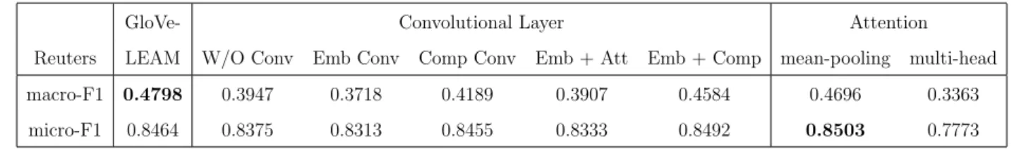
Ablative analysis
We also explore some ablative methods with the GloVe-LEAM structures, the results with the same experiment setting is compared in Table 4.4.
Firstly we consider to modify the convolution layer, and it turns out to be important to take into account the local context, as sparing it greatly affects the result. We also try to change the convolution position from the attention layer to after word embedding for a direct computation of label-phrase similarity, or use it to composite the attended single-word
(a) Training labels (b) Testing labels (c) Predicted testing labels
Figure 4.3: Reuters label correlation heatmap (subset of 50)
GloVe- Convolutional Layer Attention
Reuters LEAM W/O Conv Emb Conv Comp Conv Emb + Att Emb + Comp mean-pooling multi-head
macro-F1 0.4798 0.3947 0.3718 0.4189 0.3907 0.4584 0.4696 0.3363
micro-F1 0.8464 0.8375 0.8313 0.8455 0.8333 0.8492 0.8503 0.7773
Table 4.4: Ablative Analysis on Reuters
embeddings into the document representation, neither achieves a result as good. Moreover, adding extra convolution layer also does not boost the performance.
In LEAM we take the maximum over all label attentions assuming that each word is associated with only one label. Since it is plausible to consider each word as realted to more than one labels, we also experiment with alternative ways to compute attention. We try mean-pooling over all label attentions, and for the Reuters dataset the result makes little difference. Another possible architecture is to reserve the multiple label attention layers, and use a Binary Relavance based MLP classffier. However, the results is not as good, the reason might be that the optimization becomes harder with a larger number of parameters. It is notable that You et al. achieved an excellent performance with such multi-representation attention structure paired with bi-LSTM on datasets with more extreme label sizes [50], and it is worthwhile to explore the interaction between network structure and data characteristics in the future work.
4.4
CVDM Results and Analysis
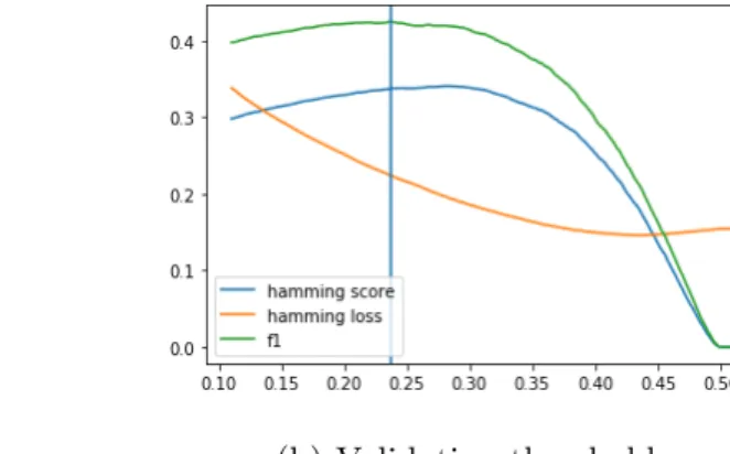
Since CVDM prediction is based on ranking loss, we compare the performances over the ROC-AUC score in sync with realted works. In order to make the final label prediction, we adopt the empirical method, that is, to find the optimal threshold on a validation set or via cross-validation if the computational power is sufficient. Figure displays a sample of threshold selection curve with maximum macro-F1 criterion, where a clear peak can be observed.
(a) Training threshold (b) Validation threshold
Figure 4.4: Empirical threshold selection on Delicious
We compare CVDM on all three datasets in Table 4.5. CVDM achieves a comparable performance to the discriminative baselines on the Delicious dataset, where the vocabulary is cleaned and stemmed for better BoW representation. Meanwhile, the model performs worse on Reuters and anon-Rev. The potential reasons can be that the their data processing is more coarse with more words reserved for more local contextual information. Moreover, CVDM may be harder to scale to a large number of labels, since a separate prior distribution is required for each label.
*CVDM and TFIDF-CVDM makes only small differences, which indicates that the prior distributions does not necessarily require concrete semantic information, but serves as an-chors that separate examples with different labels. Nevertheless, more content-relevant fea-tures can be useful when some labels are not seen during training in the situation of zero-shot or few-shot learning, where the prior network helps transfer knowledge between classes.
Reuters anon-Rev Delicious
Model Macro-AUC Micro-AUC Macro-AUC Micro-AUC Macro-AUC Micro-AUC
BoW-MLP 0.9515 0.9839 0.9138 0.9553 0.7762 0.8015
*LEAM 0.9641 0.9879 0.8917 0.9465 0.7422 0.7713
*CVDM 0.9560 0.9834 0.8416 0.9268 0.7598 0.8016
TFIDF-CVDM 0.9478 0.9820 0.8479 0.9294 0.7724 0.8107
Table 4.5: General Comparison of Results
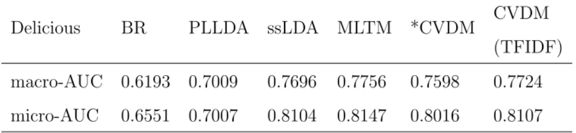
Our model is also comparable to other STOA generative models on the Delicious dataset as illustrated in Table 4.6. The models other than ours are implemented by Soleimani and Miller [33], and the code and results can be rechieved online4. They developed Multi-label Topic Model (MLTM) where each label is associated with indefinite number of latent topics, and compair it with Binary Relevance and also other supervised topic models (Partially labeled LDA, semi-supervised LDA) with different model assumptions. It is notable that these models approximate the analytical posterior estimates by Monte Carlo sampling, rather than using neural network methods. We adopt the same data preprocessing procedure and dimension of latent variable for a fair comparison.
Delicious BR PLLDA ssLDA MLTM *CVDM CVDM (TFIDF) macro-AUC 0.6193 0.7009 0.7696 0.7756 0.7598 0.7724 micro-AUC 0.6551 0.7007 0.8104 0.8147 0.8016 0.8107
Table 4.6: Comparison between generative models
We display in Table 4.7 the label semantic inferred by TFIDF-CVDM, where the words with the highest probability for each label-specific distribution (βl) are listed. Although the
top-words are mostly relevant to the label, they are also heavily influenced by high-frequency words, for example, ’use’ is ranked high for most labels. It suggests that the reconstruction
model p(X|Z) is likely not good enough. Therefore, we also try optimizing only the KL-divergence term with the margin regularizer, and the resulted macro-AUC is only about 0.1 lower than the original model. It could possibly be fixed by adjusting the weights of each term in the objective function for better optimization, and another possible improvement is to penalize the similarity between label distribution for more interpretable results.
Topic Top-words
internet use, see, page, web, document, name, type, system, click, applic writing use, make, first, write, great, comment, year, mean, thing, post reference work, free, list, take, realli, use, common, page, right, featur education one, know, read, way, design, call, good, number, com, mean
CHAPTER 5
Conclusion and Future Work
In conclusion, we study the problem of multi-label text classification, and argues that the use of annotated labels should not limit to providing supervision for the classification task, but also guiding the learning of natural language representation. We discuss two approaches specifically, and empirically show that they promote the classification performances with improved interpretability.
Label-embedding Attention Model (LEAM) learns a label-word attention layer for the composition of word embedding into document vectors. It uses a simple and efficient ar-chitecture to achieve excellent performances especially for unbalanced data, and the simple structure also provides better interpretability with the attention weights on each word. In our experiments, we analyze the architecture to explore the effect of the attention layer and the convolution layer, and demonstrate its merits in identifying multi-word expressions and capturing word-label and label-label correlations.
Conditional Variationl Document Model (CVDM) learns explicitly a probabilistic latent variable, and encourages it to contain label information by minimizing its distance to a prior distribution conditional on the label attributes, meanwhile the measure of distance - KL-divergence also serves as ranking score for prediction. The variational scheme and sampling procedure makes it more tolerant to noise, and the explicit high-level latent abstraction also provide more interpretability. Our model achieves comparable ranking performance to benchmark generative topic models, while being more flexible and generalizable with neural variational inference rather than traditional variational bayes that relies on analytic approximation.
The training of LEAM is not stable enough as certain random seed gives poor results, so cross-validation is needed in pratical use. Moreover, the effect of pre-trained word embedding could be affect by the domain of the corpus, and we have not experiment on data with more extreme number of labels (ex. over 100).
CVDM breaks down when the label amount grows, and it is possible that similar labels or hierarchical label relationship is hard to be distinguish by the separately learned latent priors and the coarse-grained BoW distribution. Another problem is that the current decision rule is not disciplined since the classification score derived from a divergence measure is not well-distributed. In addition, the topic generative model does not fit very well as we show in the experiments.
Therefore, future works may consider the following aspects:
1. Use LEAM representation with more advanced classification algorithms, and extend the experiments to extreme multi-label problems;
2. Explore variational attention mechanism on LEAM;
3. Re-construct CVAE with more realistic latent structures, such as hierarchical VAE or semi-supervised VAE;
4. Modify CVAE objective function with different topic diversity regularization or diver-gence measures such as wasserstein distance.
CHAPTER 6
Appendix
Evidence Lower Bound (ELBO)
logp(X) = log Z Z p(X,Z) = log Z Z p(X,Z)q(Z) q(Z) = log Eq p(X,Z) q(Z)
≥Eq[logp(X,Z)]−Eq[logq(Z)] = ELBO by Jensen Inequality
=Eq[logp(X)]−DKL(q(Z)kp(Z|X))
VAE Objective
logp(X) = log Z Z p(X,Z)q(Z|X) q(Z|X) = log Eq(Z|X) p(X,Z) q(Z|X) ≥Eq(Z|X)[logp(X|Z)]]−DKL(q(Z|X)kp(Z)) = LV AECVAE Objective
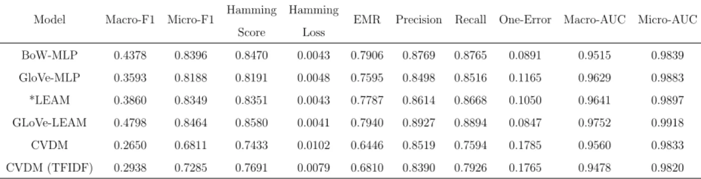
LCV AE = logp(X|A)≥Eq(Z|X,A)[logp(X|Z,A)]]−DKL(q(Z|X,A)kp(Z|A))Model Macro-F1 Micro-F1 Hamming Score
Hamming Loss
EMR Precision Recall One-Error Macro-AUC Micro-AUC BoW-MLP 0.4378 0.8396 0.8470 0.0043 0.7906 0.8769 0.8765 0.0891 0.9515 0.9839 GloVe-MLP 0.3593 0.8188 0.8191 0.0048 0.7595 0.8498 0.8516 0.1165 0.9629 0.9883 *LEAM 0.3860 0.8349 0.8351 0.0043 0.7787 0.8614 0.8668 0.1050 0.9641 0.9897 GLoVe-LEAM 0.4798 0.8464 0.8580 0.0041 0.7940 0.8927 0.8894 0.0847 0.9752 0.9918 CVDM 0.2650 0.6811 0.7433 0.0102 0.6446 0.8519 0.7594 0.1785 0.9560 0.9833 CVDM (TFIDF) 0.2938 0.7285 0.7691 0.0079 0.6810 0.8390 0.7926 0.1765 0.9478 0.9820
Table 6.1: Reuters Results
Model Macro-F1 Micro-F1 Hamming Score
Hamming Loss
EMR Precision Recall One-Error Macro-AUC Micro-AUC BoW-MLP 0.4947 0.7118 0.6770 0.0206 0.4672 0.7433 0.8059 0.1153 0.9138 0.9553 GloVe-MLP 0.3987 0.6846 0.6517 0.0232 0.4347 0.7370 0.7685 0.1454 0.8917 0.9465 *LEAM 0.5358 0.7406 0.7106 0.0192 0.4848 0.7920 0.8249 0.0921 0.9284 0.960 GLoVe-LEAM 0.5129 0.7004 0.6696 0.0226 0.4450 0.7662 0.7815 0.1278 0.9227 0.9567 CVDM 0.2955 0.5024 0.5166 0.0494 0.2985 0.7363 0.590 0.2725 0.8371 0.9261 CVDM (TFIDF) 0.2564 0.4937 0.4981 0.0485 0.2814 0.7123 0.5737 0.2963 0.9223 0.9224
Table 6.2: anon-Rev Results
Model Macro-F1 Micro-F1 Hamming Score
Hamming Loss
EMR Precision Recall One-Error Micro-AUC Macro-AUC BoW-MLP 0.4361 0.4762 0.3347 0.1486 0.0511 0.4554 0.5072 0.3899 0.7762 0.8015
*LEAM 0.3958 0.4348 0.2987 0.1639 0.0391 0.4192 0.4523 0.4621 0.7422 0.7713 CVDM 0.4182 0.4590 0.3270 0.2490 0.0138 0.6958 0.3750 0.4679 0.7598 0.8016 CVDM (TFIDF) 0.4338 0.4704 0.3354 0.2432 0.0144 0.7089 0.3810 0.4493 0.7724 0.8107
REFERENCES
[1] Felipe Almeida and Geraldo Xex´eo. Word embeddings: A survey. arXiv preprint arXiv:1901.09069, 2019.
[2] Dzmitry Bahdanau, Kyunghyun Cho, and Yoshua Bengio. Neural machine translation by jointly learning to align and translate. arXiv preprint arXiv:1409.0473, 2014. [3] Yoshua Bengio, R´ejean Ducharme, Pascal Vincent, and Christian Jauvin. A neural
probabilistic language model. Journal of machine learning research, 3(Feb):1137–1155, 2003.
[4] Kush Bhatia, Himanshu Jain, Purushottam Kar, Manik Varma, and Prateek Jain. Sparse local embeddings for extreme multi-label classification. In C. Cortes, N. D. Lawrence, D. D. Lee, M. Sugiyama, and R. Garnett, editors, Advances in Neural Infor-mation Processing Systems 28, pages 730–738. Curran Associates, Inc., 2015.
[5] David M Blei, Andrew Y Ng, and Michael I Jordan. Latent dirichlet allocation. Journal of machine Learning research, 3(Jan):993–1022, 2003.
[6] Sneha Chaudhari, Gungor Polatkan, Rohan Ramanath, and Varun Mithal. An attentive survey of attention models, 04 2019.
[7] Amanda Clare and Ross D King. Knowledge discovery in multi-label phenotype data. In European Conference on Principles of Data Mining and Knowledge Discovery, pages 42–53. Springer, 2001.
[8] Scott Deerwester, Susan T Dumais, George W Furnas, Thomas K Landauer, and Richard Harshman. Indexing by latent semantic analysis. Journal of the American society for information science, 41(6):391–407, 1990.
[9] Jacob Devlin, Ming-Wei Chang, Kenton Lee, and Kristina Toutanova. Bert: Pre-training of deep bidirectional transformers for language understanding. arXiv preprint arXiv:1810.04805, 2018.
[10] Andr´e Elisseeff and Jason Weston. A kernel method for multi-labelled classification. In
Advances in neural information processing systems, pages 681–687, 2002.
[11] Yoav Goldberg. Neural network methods for natural language processing. Synthesis Lectures on Human Language Technologies, 10(1):1–309, 2017.
[12] Zellig S Harris. Distributional structure. Word, 10(2-3):146–162, 1954.
[13] Thomas Hofmann. Probabilistic latent semantic analysis. InProceedings of the Fifteenth conference on Uncertainty in artificial intelligence, pages 289–296. Morgan Kaufmann Publishers Inc., 1999.
[14] Matthew Johnson, David K Duvenaud, Alex Wiltschko, Ryan P Adams, and Sandeep R Datta. Composing graphical models with neural networks for structured representations and fast inference. In Advances in neural information processing systems, pages 2946– 2954, 2016.
[15] Diederik P Kingma and Jimmy Ba. Adam: A method for stochastic optimization. arXiv preprint arXiv:1412.6980, 2014.
[16] Diederik P Kingma and Max Welling. Auto-encoding variational bayes. arXiv preprint arXiv:1312.6114, 2013.
[17] Gakuto Kurata, Bing Xiang, and Bowen Zhou. Improved neural network-based multi-label classification with better initialization leveraging multi-label co-occurrence. In Pro-ceedings of the 2016 Conference of the North American Chapter of the Association for Computational Linguistics: Human Language Technologies, pages 521–526, 2016. [18] Omer Levy and Yoav Goldberg. Neural word embedding as implicit matrix
factoriza-tion. In Advances in neural information processing systems, pages 2177–2185, 2014. [19] Zhouhan Lin, Minwei Feng, Cicero Nogueira dos Santos, Mo Yu, Bing Xiang, Bowen
Zhou, and Yoshua Bengio. A structured self-attentive sentence embedding. arXiv preprint arXiv:1703.03130, 2017.
[20] Yishu Miao, Edward Grefenstette, and Phil Blunsom. Discovering discrete latent topics with neural variational inference. In Proceedings of the 34th International Conference on Machine Learning-Volume 70, pages 2410–2419. JMLR. org, 2017.
[21] Yishu Miao, Lei Yu, and Phil Blunsom. Neural variational inference for text processing. In International conference on machine learning, pages 1727–1736, 2016.
[22] Tomas Mikolov, Kai Chen, Greg Corrado, and Jeffrey Dean. Efficient estimation of word representations in vector space. arXiv preprint arXiv:1301.3781, 2013.
[23] George Miller. WordNet: An electronic lexical database. MIT press, 1998.
[24] Jinseok Nam, Jungi Kim, Eneldo Loza Menc´ıa, Iryna Gurevych, and Johannes F¨urnkranz. Large-scale multi-label text classificationrevisiting neural networks. InJoint european conference on machine learning and knowledge discovery in databases, pages 437–452. Springer, 2014.
[25] Andrew Y Ng and Michael I Jordan. On discriminative vs. generative classifiers: A comparison of logistic regression and naive bayes. In Advances in neural information processing systems, pages 841–848, 2002.
[26] Jeffrey Pennington, Richard Socher, and Christopher Manning. Glove: Global vectors for word representation. In Proceedings of the 2014 conference on empirical methods in natural language processing (EMNLP), pages 1532–1543, 2014.
[27] Matthew E Peters, Mark Neumann, Mohit Iyyer, Matt Gardner, Christopher Clark, Kenton Lee, and Luke Zettlemoyer. Deep contextualized word representations. arXiv preprint arXiv:1802.05365, 2018.
[28] Yashoteja Prabhu and Manik Varma. Fastxml: A fast, accurate and stable tree-classifier for extreme multi-label learning. InProceedings of the 20th ACM SIGKDD international conference on Knowledge discovery and data mining, pages 263–272. ACM, 2014. [29] Alec Radford, Karthik Narasimhan, Tim Salimans, and Ilya Sutskever. Improving
lan-guage understanding by generative pre-training. URL https://s3-us-west-2. amazon-aws. com/openai-assets/research-covers/languageunsupervised/language understanding paper. pdf, 2018.
[30] Jesse Read, Bernhard Pfahringer, Geoff Holmes, and Eibe Frank. Classifier chains for multi-label classification. In Joint European Conference on Machine Learning and Knowledge Discovery in Databases, pages 254–269. Springer, 2009.
[31] Dinghan Shen, Guoyin Wang, Wenlin Wang, Martin Renqiang Min, Qinliang Su, Yizhe Zhang, Chunyuan Li, Ricardo Henao, and Lawrence Carin. Baseline needs more love: On simple word-embedding-based models and associated pooling mechanisms. arXiv preprint arXiv:1805.09843, 2018.
[32] Kihyuk Sohn, Honglak Lee, and Xinchen Yan. Learning structured output represen-tation using deep conditional generative models. In Advances in neural information processing systems, pages 3483–3491, 2015.
[33] Hossein Soleimani and David J Miller. Semi-supervised multi-label topic models for document classification and sentence labeling. In Proceedings of the 25th ACM Inter-national on Conference on Information and Knowledge Management, pages 105–114. ACM, 2016.
[34] Alessandro Sordoni, Michel Galley, Michael Auli, Chris Brockett, Yangfeng Ji, Mar-garet Mitchell, Jian-Yun Nie, Jianfeng Gao, and Bill Dolan. A neural network ap-proach to context-sensitive generation of conversational responses. arXiv preprint arXiv:1506.06714, 2015.
[35] Mohammad S Sorower. A literature survey on algorithms for multi-label learning. [36] Ilya Tolstikhin, Olivier Bousquet, Sylvain Gelly, and Bernhard Schoelkopf. Wasserstein
auto-encoders. arXiv preprint arXiv:1711.01558, 2017.
[37] Michael Tschannen, Olivier Bachem, and Mario Lucic. Recent advances in autoencoder-based representation learning. arXiv preprint arXiv:1812.05069, 2018.
[38] Grigorios Tsoumakas and Ioannis Katakis. www. International Journal of Data Ware-housing and Mining (IJDWM), 3(3):1–13, 2007.
[39] Grigorios Tsoumakas, Ioannis Katakis, and Ioannis Vlahavas. Mining multi-label data. In Data mining and knowledge discovery handbook, pages 667–685. Springer, 2009.
[40] Joseph Turian, Lev Ratinov, and Yoshua Bengio. Word representations: a simple and general method for semi-supervised learning. InProceedings of the 48th annual meeting of the association for computational linguistics, pages 384–394. Association for Compu-tational Linguistics, 2010.
[41] Ashish Vaswani, Noam Shazeer, Niki Parmar, Jakob Uszkoreit, Llion Jones, Aidan N Gomez, Lukasz Kaiser, and Illia Polosukhin. Attention is all you need. In Advances in neural information processing systems, pages 5998–6008, 2017.
[42] Guoyin Wang, Chunyuan Li, Wenlin Wang, Yizhe Zhang, Dinghan Shen, Xinyuan Zhang, Ricardo Henao, and Lawrence Carin. Joint embedding of words and labels for text classification. arXiv preprint arXiv:1805.04174, 2018.
[43] Wenlin Wang, Yunchen Pu, Vinay Kumar Verma, Kai Fan, Yizhe Zhang, Changyou Chen, Piyush Rai, and Lawrence Carin. Zero-shot learning via class-conditioned deep generative models. In Thirty-Second AAAI Conference on Artificial Intelligence, 2018. [44] Yunchao Wei, Wei Xia, Junshi Huang, Bingbing ni, Jian Dong, Yao Zhao, and Shuicheng
Yan. Cnn: Single-label to multi-label. 06 2014.
[45] John Wieting, Mohit Bansal, Kevin Gimpel, and Karen Livescu. Towards universal paraphrastic sentence embeddings. arXiv preprint arXiv:1511.08198, 2015.
[46] David Arthur Wilkins. Linguistics in language teaching. E. Arnold, 1973, 1972.
[47] Xinchen Yan, Jimei Yang, Kihyuk Sohn, and Honglak Lee. Attribute2image: Condi-tional image generation from visual attributes. In European Conference on Computer Vision, pages 776–791. Springer, 2016.
[48] Pengcheng Yang, Xu Sun, Wei Li, Shuming Ma, Wei Wu, and Houfeng Wang. Sgm: sequence generation model for multi-label classification. In Proceedings of the 27th International Conference on Computational Linguistics, pages 3915–3926, 2018.
[49] Zichao Yang, Diyi Yang, Chris Dyer, Xiaodong He, Alex Smola, and Eduard Hovy. Hierarchical attention networks for document classification. In Proceedings of the 2016 Conference of the North American Chapter of the Association for Computational Lin-guistics: Human Language Technologies, pages 1480–1489, 2016.
[50] Ronghui You, Suyang Dai, Zihan Zhang, Hiroshi Mamitsuka, and Shanfeng Zhu. At-tentionxml: Extreme multi-label text classification with multi-label attention based recurrent neural networks. arXiv preprint arXiv:1811.01727, 2018.
[51] Min-Ling Zhang and Zhi-Hua Zhou. Multilabel neural networks with applications to functional genomics and text categorization. IEEE transactions on Knowledge and Data Engineering, 18(10):1338–1351, 2006.
[52] Min-Ling Zhang and Zhi-Hua Zhou. Ml-knn: A lazy learning approach to multi-label learning. Pattern recognition, 40(7):2038–2048, 2007.
[53] Xiang Zhang, Junbo Zhao, and Yann LeCun. Character-level convolutional networks for text classification. In Advances in neural information processing systems, pages 649–657, 2015.
[54] Shengjia Zhao, Jiaming Song, and Stefano Ermon. Infovae: Information maximizing variational autoencoders. arXiv preprint arXiv:1706.02262, 2017.
[55] Tiancheng Zhao, Ran Zhao, and Maxine Eskenazi. Learning discourse-level diversity for neural dialog models using conditional variational autoencoders. arXiv preprint arXiv:1703.10960, 2017.
[56] Arkaitz Zubiaga, Alberto P Garc´ıa-Plaza, V´ıctor Fresno, and Raquel Mart´ınez. Content-based clustering for tag cloud visualization. In 2009 International Conference on Advances in Social Network Analysis and Mining, pages 316–319. IEEE, 2009.