R E S E A R C H A R T I C L E
Open Access
Random forest versus logistic regression:
a large-scale benchmark experiment
Raphael Couronné
*, Philipp Probst and Anne-Laure Boulesteix
Abstract
Background and goal: The Random Forest (RF) algorithm for regression and classification has considerably gained popularity since its introduction in 2001. Meanwhile, it has grown to a standard classification approach competing with logistic regression in many innovation-friendly scientific fields.
Results: In this context, we present a large scale benchmarking experiment based on 243 real datasets comparing the prediction performance of the original version of RF with default parameters and LR as binary classification tools. Most importantly, the design of our benchmark experiment is inspired from clinical trial methodology, thus avoiding common pitfalls and major sources of biases.
Conclusion: RF performed better than LR according to the considered accuracy measured in approximately 69% of the datasets. The mean difference between RF and LR was 0.029 (95%-CI=[ 0.022, 0.038]) for the accuracy, 0.041 (95%-CI=[ 0.031, 0.053]) for the Area Under the Curve, and−0.027 (95%-CI=[−0.034,−0.021]) for the Brier score, all measures thus suggesting a significantly better performance of RF. As a side-result of our benchmarking experiment, we observed that the results were noticeably dependent on the inclusion criteria used to select the example datasets, thus emphasizing the importance of clear statements regarding this dataset selection process. We also stress that neutral studies similar to ours, based on a high number of datasets and carefully designed, will be necessary in the future to evaluate further variants, implementations or parameters of random forests which may yield improved accuracy compared to the original version with default values.
Keywords: Logistic regression, Classification, Prediction, Comparison study
Introduction
In the context of low-dimensional data (i.e. when the num-ber of covariates is small compared to the sample size), logistic regression is considered a standard approach for binary classification. This is especially true in scientific fields such as medicine or psycho-social sciences where the focus is not only on prediction but also on explana-tion; see Shmueli [1] for a discussion of this distinction. Since its invention 17 years ago, the random forest (RF) prediction algorithm [2], which focuses on prediction rather than explanation, has strongly gained popularity and is increasingly becoming a common “standard tool” also used by scientists without any strong background in statistics or machine learning. Our experience as authors, reviewers and readers is that random forest can now be *Correspondence:[email protected]
Department of Medical Information Processing, Biometry and Epidemiology, LMU Munich, Marchioninistr. 15, 81377 Munich, Germany
used routinely in many scientific fields without particular justification and without the audience strongly question-ing this choice. While its use was in the early years limited to innovation-friendly scientists interested (or experts) in machine learning, random forests are now more and more well-known in various non-computational communities.
In this context, we believe that the performance of RF should be systematically investigated in a large-scale benchmarking experiment and compared to the cur-rent standard: logistic regression (LR). We make the— admittedly somewhat controversial—choice to consider the standard version of RF only with default parame-ters — as implemented in the widely used R package randomForest[3] version 4.6-12 — and logistic regres-sion only as the standard approach which is very often used for low dimensional binary classification.
The rationale behind this simplifying choice is that, to become a “standard method” that users with differ-ent (possibly non-computational) backgrounds select by
© The Author(s). 2018Open AccessThis article is distributed under the terms of the Creative Commons Attribution 4.0 International License (http://creativecommons.org/licenses/by/4.0/), which permits unrestricted use, distribution, and reproduction in any medium, provided you give appropriate credit to the original author(s) and the source, provide a link to the Creative Commons license, and indicate if changes were made. The Creative Commons Public Domain Dedication waiver (http://creativecommons.org/publicdomain/zero/1.0/) applies to the data made available in this article, unless otherwise stated.
default, a method should be simple to use and not require any complex human intervention (such as parameter tun-ing) demanding particular expertise. Our experience from statistical consulting is that applied research practitioners tend to apply methods in their simplest form for differ-ent reasons including lack of time, lack of expertise and the (critical) requirement of many applied journals to keep data analysis as simple as possible. Currently, the simplest approach consists of running RF with default parameter values, since no unified and easy-to-use tuning approach has yet established itself. It is not the goal of this paper to discuss how to improve RF’s performance by appro-priate tuning strategies and which level of expertise is ideally required to use RF. We simply acknowledge that the standard variant with default values is widely used and conjecture that things will probably not dramatically change in the short term. That is why we made the choice to consider RF with default values as implemented in the very widely used packagerandomForest—while admit-ting that, if time and competence are available, more sophisticated strategies may often be preferable. As an outlook, we also consider RF with parameters tuned using the recent packagetuneRanger[4] in a small additional study.
Comparison studies published in literature often include a large number of methods but a relatively small number of datasets [5], yielding an ill-posed problem as far as statistical interpretation of benchmarking results are concerned. In the present paper we take an oppo-site approach: we focus on only two methods for the reasons outlined above but design our benchmarking experiments in such a way that it yields solid evidence. A particular strength of our study is that we as authors are equally familiar with both methods. Moreover, we are “neutral” in the sense that we have no personal pri-oripreference for one of the methods: ALB published a number of papers on RF, but also papers on regression-based approaches [6, 7] and papers pointing to critical problems of RF [8–10]. Neutrality and equal expertise would be much more difficult if not impossible to ensure if several variants of RF (including tuning strategies) and logistic regression were included in the study. Further dis-cussions of the concept of authors’ neutrality can be found elsewhere [5,11].
Most importantly, the design of our benchmark exper-iment is inspired by the methodology of clinical trials that has been developed with huge efforts for several decades. We follow the line taken in our recent paper [11] and carefully define the design of our benchmark experiments including, beyond issues related to neutrality outlined above, considerations on sample size (i.e. number of datasets included in the experiment) and inclusion cri-teria for datasets. Moreover, as an analogue to subgroup analyses and the search for biomarkers of treatment effect
in clinical trials, we also investigate the dependence of our conclusions on datasets’ characteristics.
As an important by-product of our study, we provide empirical insights into the importance of inclusion crite-ria for datasets in benchmarking experiments and general critical discussions on design issues and scientific prac-tice in this context. The goal of our paper is thus two-fold. Firstly we aim to present solid evidence on the perfor-mance of standard logistic regression and random forests with default values. Secondly, we demonstrate the design of a benchmark experiment inspired from clinical trial methodology.
The rest of this paper is structured as follows. After a short overview of LR and RF, the associated VIM, par-tial dependence plots [12], the cross-validation procedure and performance measures used to evaluate the meth-ods (“Background” section), we present our benchmark-ing approach in “Methods” section, including the criteria for dataset selection. Results are presented in “Results” section.
Background
This section gives a short overview of the (existing) meth-ods involved in our benchmarking experiments: logistic regression (LR), random forest (RF) including variable importance measures, partial dependence plots, and per-formance evaluation by cross-validation using different performance measures.
Logistic regression (LR)
LetY denote the binary response variable of interest and X1,. . .,Xp the random variables considered as
explain-ing variables, termed featuresin this paper. The logistic regression model links the conditional probabilityP(Y = 1|X1, ...,Xp)toX1,. . .,Xpthrough P(Y=1|X1, ...,Xp)= expβ0+β1X1+ · · · +βpXp 1+expβ0+β1X1+ · · · +βpXp , (1) whereβ0,β1,. . .,βpare regression coefficients, which are
estimated by maximum-likelihood from the considered dataset. The probability that Y = 1 for a new instance is then estimated by replacing the β’s by their estimated counterparts and theX’s by their realizations for the con-sidered new instance in Eq. (1). The new instance is then assigned to classY =1 ifP(Y =1) >c, wherecis a fixed threshold, and to classY = 0 otherwise. The commonly used thresholdc = 0.5, which is also used in our study, yields a so-called Bayes classifier. As for all model-based methods, the prediction performance of LR depends on whether the data follow the assumed model. In contrast, the RF method presented in the next section does not rely on any model.
Random forest (RF)
Brief overview
The random forest (RF) is an “ensemble learning” tech-nique consisting of the aggregation of a large number of decision trees, resulting in a reduction of variance compared to the single decision trees. In this paper we consider Leo Breiman’s original version of RF [2], while acknowledging that other variants exist, for example RF based on conditional inference trees [13] which address the problem of variable selection bias [14] and perform better in some cases, or extremely randomized trees [15].
In the original version of RF [2], each tree of the RF is built based on a bootstrap sample drawn randomly from the original dataset using the CART method and the Decrease Gini Impuritiy (DGI) as the splitting criterion [2]. When building each tree, at each split, only a given numbermtryof randomly selected features are consid-ered as candidates for splitting. RF is usually considconsid-ered a black-box algorithm, as gaining insight on a RF predic-tion rule is hard due to the large number of trees. One of the most common approaches to extract from the ran-dom forest interpretable information on the contribution of different variables consists in the computation of the so-called variable importance measures outlined in “Variable importance measures” section. In this study we use the packagerandomForest[3] (version 4.6-12) with default values, see the next paragraph for more details on tuning parameters.
Hyperparameters
This section presents the most important parameters for RF and their common default values as implemented in the R packagerandomForest[3] and considered in our study. Note, however, that alternative choices may yield better performance [16, 17] and that parameter tuning for RF has to be further addressed in future research. The parameterntreedenotes the number of trees in the forest. Strictly speaking,ntreeis not a tuning parame-ter (see [18] for more insight into this issue) and should be in principle as large as possible so that each candi-date feature has enough opportunities to be selected. In practice, however, performance reaches a plateau with a few hundreds of trees for most datasets [18]. The default value is ntree=500 in the package randomForest. The parametermtrydenotes the number of features ran-domly selected as candidate features at each split. A low value increases the chance of selection of features with small effects, which may contribute to improved predic-tion performance in cases where they would otherwise be masked by features with large effects. A high value ofmtryreduces the risk of having only non-informative candidate features. In the packagerandomForest, the default value is √p for classification with p the num-ber of features of the dataset. The parameternodesize
represents the minimum size of terminal nodes. Setting this number larger yields smaller trees. The default value is 1 for classification. The parameterreplacerefers to the resampling scheme used to randomly draw from the original dataset different samples on which the trees are grown. The default is replace=TRUE, yielding boot-strap samples, as opposed toreplace=FALSEyielding subsamples— whose size is determined by the parameter sampsize.
The performance of RF is known to be relatively robust against parameter specifications: performance generally depends less on parameter values than for other machine learning algorithms [19]. However, noticeable improve-ments may be achieved in some cases [20]. The recent R packagetuneRanger[4] allows to automatically tune RF’s parameters simultaneously using an efficient model-based optimization procedure. In additional analyses pre-sented in “Additional analysis: tuned RF” section, we compare the performance of RF and LR with the perfor-mance of RF tuned with this procedure (denoted as TRF).
Variable importance measures
As a byproduct of random forests, the built-in vari-able importance measures (VIM) rank thevariables (i.e. the features) with respect to their relevance for pre-diction [2]. The so-called Gini VIM has shown to be strongly biased [14]. The second common VIM, called permutation-based VIM, is directly based on the accu-racy of RF: it is computed as the mean difference (over the ntree trees) between the OOB errors before and after randomly permuting the values of the consid-ered variable. The underlying idea is that the permu-tation of an important feature is expected to decrease accuracy more strongly than the permutation of an unimportant variable.
VIMs are not sufficient in capturing the patterns of dependency between features and response. They only reflect—in the form of a single number—the strength of this dependency. Partial dependence plots can be used to address this shortcoming. They can essentially be applied to any prediction method but are particularly useful for black-box methods which (in contrast to, say, generalized linear models) yield less interpretable results.
Partial dependence plots
Partial dependence plots (PDPs) offer insight of any black box machine learning model, visualizing how each feature influences the prediction while averaging with respect to all the other features. The PDP method was first devel-oped for gradient boosting [12]. LetFdenote the function associated with the classification rule: for classification, FX1,. . .,Xp
∈ [0, 1] is the predicted probability of the observation belonging to class 1. Let j be the index of the chosen featureXj andXj its complement, such that
Xj=X1, ...,Xj−1,Xj+1, ...,Xp
. The partial dependence of Fon featureXjis the expectation
FXj =EXjF
Xj,Xj
(2) which can be estimated from the data using the empirical distribution ˆ pXj(x)= 1 N N i=1 Fxi,1, ...xi,j−1,x,xi,j+1, ...,xi,p , (3) where xi,1,. . .,xi,p stand for the observed values of
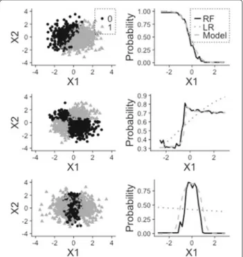
X1,. . .,Xpfor theith observation. As an illustration, we
display in Fig. 1 the partial dependence plots obtained by logistic regression and random forest for three simu-lated datasets representing classification problems, each includingn = 1000 independent observations. For each dataset the variableY is simulated according to the for-mula log(P(Y = 1)/P(Y = 0)) = β0+β1X1+β2X2+ β3X1X2+β4X12. The first dataset (top) represents the
lin-ear scenario (β1 = 0,β2 = 0,β3 = β4 = 0), the second
dataset (middle) an interaction (β1 =0,β2 =0,β3 =0, β4 = 0) and the third (bottom) a case of non-linearity
(β1=β2=β3=0,β4=0). For all three datasets the
ran-dom vector(X1,X2)follows distributionN2(0,I), withI
representing the identity matrix. The data points are rep-resented in the left column, while the PDPs are displayed
Fig. 1Example of partial dependence plots. Plot of the PDP for the three simulated datasets. Each line is related to a dataset. On the left, visualization of the dataset. On the right, the partial dependence for the variableX1. First dataset:β0=1,β1=5,β2= −2 (linear), second dataset:β0=1,β1=1,β2= −1,β3=3 (interaction), third dataset
β0= −2,β4=5 (non-linear)
in the right column for RF, logistic regression as well as the true logistic regression model (i.e. with the true coefficient values instead of fitted values). We see that RF captures the dependence and non-linearity structures in cases 2 and 3, while logistic regression, as expected, is not able to. Performance assessment
Cross-validation
In a k-fold cross-validation (CV), the original dataset is randomly partitioned intok subsets of approximately equal sizes. At each of the k CV iterations, one of the folds is chosen as the test set, while thek−1 others are used for training. The considered performance measure is computed based on the test set. After thekiterations, the performances are finally averaged over the iterations. In our study, we perform 10 repetitions of stratified 5-fold CV, as commonly recommended [21]. In the stratified ver-sion of the CV, the folds are chosen such that the class frequencies are approximately the same in all folds. The stratified version is chosen mainly to avoid problems with strongly imbalanced datasets occurring when all obser-vations of a rare class are included in the same fold. By “10 repetitions”, we mean that the whole CV procedure is repeated for 10 random partitions intokfolds with the aim to provide more stable estimates.
In our study, this procedure is applied to different per-formance measures outlined in the next subsection, for LR and RF successively and forMreal datasets successively. For each performance measure, the results are stored in form of anM×2 matrix.
Performance measures
Given a classifier and a test dataset of size ntest, let pˆi,
i = 1,. . .,ndenote the estimated probability of the ith observation (i = 1,. . .,ntest) to belong to classY = 1,
while the true class membership of observationiis simply denoted asyi. Following the Bayes rule implicitly adopted
in LR and RF, the predicted classyˆi is simply defined as ˆ
yi=1 ifpˆi>0.5 and 0 otherwise.
The accuracy, or proportion of correct predictions is estimated as acc= 1 ntest ntest i=1 Iyi= ˆyi ,
whereI(.)denotes the indicator function (I(A) = 1 ifA holds,I(A)=0 otherwise). TheArea Under Curve(AUC), or probability that the classifier ranks a randomly chosen observation withY = 1 higher than a randomly chosen observation withY=0 is estimated as
auc= 1 n0,testn1,test i:yi=1 j:yj=0 Ipˆi>pˆj ,
where n0,test andn1,test are the numbers of observations
The Brier score is a commonly and increasingly used performance measure [22, 23]. It measures the devia-tion between true class and predicted probability and is estimated as brier= 1 ntest ntest i=1 ˆ pi−yi 2 . Methods
The OpenML database
So far we have stated that the benchmarking experi-ment uses a collection ofMreal datasets without further specifications. In practice, one often uses already for-matted datasets from public databases. Some of these databases offer a user-friendly interface and good doc-umentation which facilitate to some extent the prelimi-nary steps of the benchmarking experiment (search for datasets, data download, preprocessing). One of the most well-known database is the UCI repository [24]. Specific scientific areas may have their own databases, such as ArrayExpress for molecular data from high-throughput experiments [25]. More recently, the OpenML database [26] has been initiated as an exchange platform allow-ing machine learnallow-ing scientists to share their data and results. This database included as many as 19660 datasets in October 2016 when we selected datasets to initiate our study, a non-negligible proportion of which are rele-vant as example datasets for benchmarking classification methods.
Inclusion criteria and subgroup analyses
When using a huge database of datasets, it becomes obvi-ous that one has to define criteria for inclusion in the benchmarking experiment. Inclusion criteria in this con-text do not have any long tradition in computational science. The criteria used by researchers—including our-selves before the present study—to select datasets are most often completely non-transparent. It is often the fact that they select a number of datasets which were found to somehow fit the scope of the investigated methods, but without clear definition of this scope.
We conjecture that, from published studies, datasets are occasionally removed from the experiment a pos-teriori because the results do not meet the expecta-tions/hopes of the researchers. While the vast majority of researchers certainly do not cheat consciously, such prac-tices may substantially introduce bias to the conclusion of a benchmarking experiment; see previous literature [27] for theoretical and empirical investigation of this prob-lem. Therefore, “fishing for datasets” after completion of the benchmark experiment should be prohibited, see Rule 4 of the “ten simple rules for reducing over-optimistic reporting” [28].
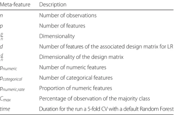
Independent of the problem of fishing for significance, it is important that the criteria for inclusion in the bench-marking experiment are clearly stated as recently dis-cussed [11]. In our study, we consider simple datasets’ characteristics, also termed “meta-features”. They are pre-sented in Table1. Based on these datasets’ characteristics, we define subgroups and repeat the benchmark study within these subgroups, following the principle of sub-group analyses in clinical research. For example, one could analyse the results for “large” datasets (n > 1000) and “small datasets” (n ≤ 1000) separately. Moreover, we also examine the subgroup of datasets related to bio-sciences/medicine.
Meta-learning
Taking another perspective on the problem of benchmark-ing results bebenchmark-ing dependent on dataset’s meta-features, we also consider modelling the difference between the meth-ods’ performances (considered as response variable) based on the datasets’ meta-features (considered as features). Such a modelling approach can be seen as a simple form ofmeta-learning—a well-known task in machine learning [29]. A similar approach using linear mixed models has been recently applied to the selection of an appropriate classification method in the context of high-dimensional gene expression data analysis [30]. Considering the poten-tially complex dependency patterns between response and features, we use RF as a prediction tool for this purpose. Power calculation
Considering theM×2 matrix, collecting the performance measures for the two investigated methods (LR and RF) on theMconsidered datasets, one can perform a test for paired samples to compare the performances of the two methods [31]. We refer to the previously published statis-tical framework [31] for a precise mathematical definition of the tested null-hypothesis in the case of the t-test for paired samples. In this framework, the datasets play the
Table 1Considered meta-features
Meta-feature Description
n Number of observations p Number of features
p
n Dimensionality
d Number of features of the associated design matrix for LR
d
n Dimensionality of the design matrix
pnumeric Number of numeric features
pcategorical Number of categorical features
pnumeric,rate Proportion of numeric features
Cmax Percentage of observation of the majority class
role of thei.i.d.observations used for the t-test. Sample size calculations for the t-test for paired samples can give an indication of the rough number of datasets required to detect a given differenceδin performances considered as relevant for a given significance level (e.g.,α = 0.05) and a given power (e.g., 1−β = 0.8). For large numbers and a two-sided test, the required number of datasets can be approximated as
Mreq≈
z1−α/2+z1−β2σ2
δ2 (4)
where zq is the q-quantile of the normal distribution
and σ2 is the variance of the difference between the two methods’ performances over the datasets, which may be roughly estimated through a pilot study or previous literature.
For example, the required number of datasets to detect a difference in performances ofδ = 0.05 withα = 0.05 and 1−β = 0.8 isMreq =32 if we assume a variance of
σ2 =0.01 andM
req = 8 forσ2= 0.0025. It increases to
Mreq=197 andMreq=50, respectively, for differences of
δ=0.02.
Availability of data and materials
Several R packages are used to implement the bench-marking study:mlr(version 2.10) for higher abstraction and a simpler way to conduct benchmark studies [32], OpenML(version 1.2) for loading the datasets [33], and batchtools(version 0.9.2) for parallel computing [34]. Note that the LR and RF learners called via mlr are wrappers on the functions glm and randomForest, respectively.
The datasets supporting the conclusions of this arti-cle are freely available in OpenML as described in “The OpenML database” section.
Emphasis is placed on the reproducibility of our results. Firstly, the code implementing all our analyses is fully available from GitHub [35]. For visualization-only pur-poses, the benchmarking results are available from this link, so that our graphics can be quickly generated by mouse-click. However, the code to re-compute these results, i.e. to conduct the benchmarking study, is also available from GitHub. Secondly, since we use specific versions of R and add-on packages and our results may thus be difficult to reproduce in the future due to soft-ware updates, we also provide a docker image [36]. Docker automates the deployment of applications inside a so called “Docker container” [37]. We use it to create an R environment with all the packages we need in their cor-rect version. Note that docker is not necessary here (since all our codes are available from GitHub), but very practical for a reproducible environment and thus for reproducible research in the long term.
Results
In our study we consider a set ofMdatasets (see “Included datasets” section for more details) and compute for each of them the performance of random forest and logistic regression according to the three performance measures outlined in “Performance assessment” section.
Included datasets
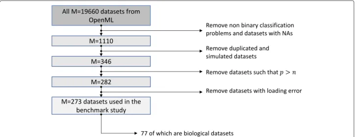
From approximately 20000 datasets currently available from OpenML [26], we select those featuring binary clas-sification problems. Further, we remove the datasets that include missing values, the obviously simulated datasets as well as duplicated datasets. We also remove datasets with more features than observations (p > n), and datasets with loading errors. This leaves us with a total of 273 datasets. See Fig.2for an overview.
Missing values due to errors
Out of the 273 selected datasets, 8 require too much com-puting time when parallelized using the package batch-tools and expired or failed. These—extremely large— datasets are discarded in the rest of the study, leaving us with 265 datasets.
Both LR and RF fail in the presence of categorical fea-tures with too many categories. More precisely, RF fails when more than 53 categories are detected in at least one of the features, while LR fails when levels undetected dur-ing the traindur-ing phase occur in the test data. We could admittedly have prevented these errors through basic pre-processing of the data such as the removal or recoding of the features that induce errors. However, we decide to just remove the datasets resulting in NAs because we do not want to address preprocessing steps, which would be a topic on their own and cannot be adequately treated along the way for such a high number of datasets. Since 22 datasets yield NAs, our study finally includes 265-22=243 datasets.
Main results
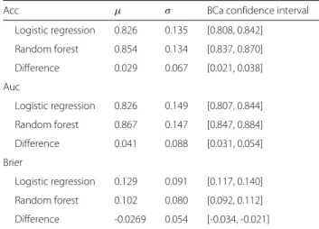
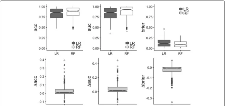
Overall performances are presented in a synthesized form in Table 2 for all three measures in form of average performances along with standard deviations and confi-dence intervals computed using the adjusted bootstrap percentile (BCa) method [38]. The boxplots of perfor-mances of Random Forest (RF) and Logistic Regression (LR) for the three considered performance measures are depicted in Fig.3, which also includes the boxplot of the difference in performances (bottom row). It can be seen from Fig.3 that RF performs better for the majority of datasets (69.0% of the datasets foracc, 72.3% foraucand
Table 2Performances of LR and RF (top: accuracy, middle: AUC, bottom: Brier score): (top: accuracy, middle: AUC, bottom: Brier score): mean performanceμ, standard deviationσand confidence interval for the mean (estimated via the bootstrap BCa method [38]) on the 243 datasets
Acc μ σ BCa confidence interval
Logistic regression 0.826 0.135 [0.808, 0.842] Random forest 0.854 0.134 [0.837, 0.870] Difference 0.029 0.067 [0.021, 0.038] Auc Logistic regression 0.826 0.149 [0.807, 0.844] Random forest 0.867 0.147 [0.847, 0.884] Difference 0.041 0.088 [0.031, 0.054] Brier Logistic regression 0.129 0.091 [0.117, 0.140] Random forest 0.102 0.080 [0.092, 0.112] Difference -0.0269 0.054 [-0.034, -0.021]
71.5% forbrier). Furthermore, when LR outperforms RF the difference is small. It can also be noted that the differ-ences in performance tend to be larger foraucthan foracc andbrier.
Explaining differences: datasets’ meta-features
In this section, we now perform different types of additional analyses with the aim to investigate the relation between the datasets’ meta-features and the performance difference between LR and RF. In “Preliminary analysis” section, we first consider an exam-ple dataset in detail to examine whether changing the sample sizenand the numberpof features for this given dataset changes the difference between performances of LR and RF (focusing on a specific dataset, we are sure that confounding is not an issue). In “Subgroup analy-ses: meta-features” to “Meta-learning” sections, we then assess the association between dataset’s meta-features and performance difference over all datasets included in our study.
Preliminary analysis
While it is obvious to any computational scientist that the performance of methods may depend on meta-features, this issue is not easy to investigate in real data settings because i) it requires a large number of datasets—a condi-tion that is often not fulfilled in practice; ii) this problem is enhanced by the correlations between meta-features. In our benchmarking experiment, however, we consider such a huge number of datasets that an investigation of the rela-tionship between methods’ performances and datasets’ characteristic becomes possible to some extent.
As a preliminary, let us illustrate this idea using only one (large) biomedical dataset, the OpenML dataset with ID= 310 includingn0=11183 observations andp0=7
features. A total of N = 50 sub-datasets are extracted from this dataset by randomly picking a numbern <n0
of observations or a numberp <p0of features. Thereby
we successively set n to n = 5.102, 103, 5.103, 104 and ptop = 1, 2, 3, 4, 5, 6. Figure4displays the boxplots of the accuracy of RF (white) and LR (dark) for varyingn (top-left) and varyingp(top-right). Each boxplot repre-sentsN = 50 data points. It can be seen from Fig.4that the accuracy increases withp for both LR and RF. This reflects the fact that relevant features may be missing from the considered random subsets of p features. Interest-ingly, it can also be seen that the increase of accuracy with pis more pronounced for RF than for LR. This supports the commonly formulated assumption that RF copes bet-ter with large numbers of features. As a consequence, the difference between RF and LR (bottom-right) increases withpfrom negative values (LR better than RF) to posi-tive values (RF better than LR). In contrast, asnincreases the performances of RF and LR increase slightly but quite
Fig. 3Main results of the benchmark experiment. Boxplots of the performance for the three considered measures on the 243 considered datasets. Top: boxplot of the performance of LR (dark) and RF (white) for each performance measure. Bottom: boxplot of the difference of performances
perf=perfRF−perfLR
Fig. 4Influence ofnandp: subsampling experiment based on dataset ID=310. Top: Boxplot of the performance (acc) of RF (dark) and LR (white) for N=50 sub-datasets extracted from the OpenML dataset with ID=310 by randomly pickingn≤nobservations andp<pfeatures. Bottom: Boxplot of the differences in performancesacc=AccRF−AccLRbetween RF and LR.p∈ {1, 2, 3, 4, 5, 6}.n∈ {5e2, 1e3, 5e3, 1e4}. Performance is
similarly (yielding a relatively stable difference), while— as expected—their variances decrease; see the left column of Fig.4.
Subgroup analyses: meta-features
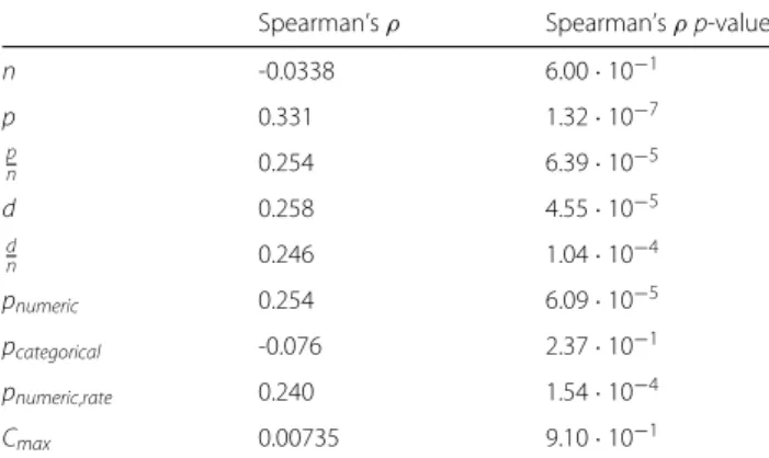
To further explore this issue over all 243 investigated datasets, we compute Spearman’s correlation coefficient between the difference in accuracy between random for-est and logistic regression (acc) and various datasets’ meta-features. The results of Spearman’s correlation test are shown in Table3. These analyses again point to the importance of the number p of features (and related meta-features), while the dataset size n is not signif-icantly correlated with acc. The percentage Cmax of
observations in the majority class, which was identified as influencing the relative performance of RF and LR in a previous study [39] conducted on a dataset from the field of political science is also not significantly correlated with accin our study. Note that our results are aver-aged over a large number of different datasets: they are not incompatible with the existence of an effect in some cases.
To investigate these dependencies more deeply, we examine the performances of RF and LR within subgroups of datasets defined based on datasets’ meta-features (called meta-features from now on), following the princi-ple of subgroup analyses well-known in clinical research. As some of the meta-features displayed in Table 3 are mutually (highly) correlated, we cluster them using a hier-archical clustering algorithm (data not shown). From the resulting dendogram we decide to select the meta-features p, n, np, Cmax, while other meta-features are considered
redundant and ignored in further analyses.
Figure5displays the boxplots of the differences in accu-racy for different subgroups based on the four selected meta-featuresp,n,pnandCmax. For each of the four
meta-features, subgroups are defined based on different cut-off values, denoted ast, successively. The histograms of the four meta-features for the 243 datasets are depicted in the
Table 3Correlation betweenaccand dataset’s features
Spearman’sρ Spearman’sρp-value
n -0.0338 6.00·10−1 p 0.331 1.32·10−7 p n 0.254 6.39·10−5 d 0.258 4.55·10−5 d n 0.246 1.04·10−4 pnumeric 0.254 6.09·10−5 pcategorical -0.076 2.37·10−1 pnumeric,rate 0.240 1.54·10−4 Cmax 0.00735 9.10·10−1
bottom row of the figure, where the considered cutoff val-ues are materialized as vertical lines. Similar pictures are obtained for the two alternative performance measures aucandbrier; See Additional file1.
It can be observed from Fig.5 that RF tends to yield better results than LR for a low n, and that the differ-ence decreases with increasingn. In contrast, RF performs comparatively poorly for datasets withp < 5, but better than LR for datasets withp ≥ 5. This is due to low per-formances of RF on a high proportion of the datasets with p< 5. For pn, the difference between RF and LR is negli-gible in low dimensionpn <0.01, but increases with the dimension. The contrast is particularly striking between the subgroupspn <0.1 (yielding a smallacc) andpn ≥0.1 (yielding a highacc), again confirming the hypothesis that the superiority of RF over LR is more pronounced for larger dimensions.
Note, however, that all these results should be inter-preted with caution, since confounding may be an issue.
Subgroup analyses: substantive context
Furthermore, we conduct additional subgroup analyses focusing on the subgroup of datasets from the field of biosciences/medicine. Out of the 243 datasets consid-ered so far, 67 are related to this field. The modified versions of Figs.3and5and Table2(as well as Fig.6 dis-cussed in “Meta-learning” section) obtained based on the subgroup formed by datasets from biosciences/medicine are displayed in Additional file 2. The outperformance of RF over LR is only slightly lower for datasets from biosciences/medicine than for the other datasets: the difference between datasets from biosciences/medicine and datasets from other fields is not significantly dif-ferent from 0. Note that one may expect bigger differ-ences between specific subfields of bioscidiffer-ences/medicine (depending on the considered prediction task). Such investigations, however, would require subject matter knowledge on each of these tasks. They could be con-ducted in future studies by experts of the respective tasks; see also the “Discussion” section.
Meta-learning
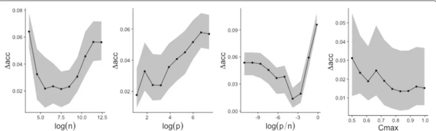
The previous section showed that benchmarking results in subgroups may be considerably different from that of the entire datasets collection. Going one step further, one can extend the analysis of features towards meta-learning to gain insight on their influence. More precisely, taking the datasets as observations we build a regression RF that predicts the difference in performance between RF and LR based on the four meta-features considered in the previous subsection p,n,pnandCmax
. Figure 6 depicts partial dependence plots for visualization of the influence of each meta-feature. Again, we notice a depen-dency on p and pn as outlined in “Subgroup analyses:
Fig. 5Subgroup analyses. Top: for each of the four selected meta-featuresn,p,p/nandCmax, boxplots ofaccfor different thresholds as criteria for
dataset selection. Bottom: distribution of the four meta-features (log scale), where the chosen thresholds are displayed as vertical lines. Note that outliers are not shown here for a more convenient visualization. For a corresponding figure including the outliers as well as the results foraucand brier, see Additional file1
meta-features” section and the comparatively bad results of RF when compared to LR for datasets with smallp. The importance ofCmaxandnis less noticeable.
Although these results should be considered with cau-tion, since they are possibly highly dependent on the particular distribution of the meta-features over the 243 datasets and confounding may be an issue, we conclude from “Explaining differences: datasets’ meta-features” section that meta-features substantially affectacc. This
points out the importance of the definition of clear inclu-sion criteria for datasets in a benchmark experiment and of the consideration of the meta-features’ distributions. Explaining differences: partial dependence plots
In the previous section we investigated the impact of datasets’ meta-features on the results of benchmarking and modeled the difference between methods’ perfor-mance based on these meta-features. In this section, we
Fig. 6Plot of the partial dependence for the 4 considered meta-features :log(n),log(p),logpn,Cmax. Thelogscale was chosen for 3 of the 4
features to obtain more uniform distribution (see Fig.5where the distribution is plotted inlogscale). For each plot, the black line denotes the median of the individual partial dependences, and the lower and upper curves of the grey regions represent respectively the 25%- und 75%-quantiles. Estimated mse is 0.00382 via a 5-CV repeated 4 times
take a different approach for the explanation of differ-ences. We use partial dependence plots as a technique to assess the dependency pattern between response and fea-tures underlying the prediction rule. More precisely, the aim of these additional analyses is to assess whether dif-ferences in performances (between LR and RF) are related to differences in partial dependence plots. After getting a global picture for all datasets included in our study, we inspect three interesting “extreme cases” more closely. In a nutshell, we observe no strong correlation between the difference in performances and the difference in par-tial dependences over the 243 considered datasets. More details are given in Additional file3: in particular, we see in the third example dataset that, as expected from the theory, RF performs better than LR in the presence of a non-linear dependence pattern between features and response.
Additional analysis: tuned RF
As an outlook, a third method is compared to RF and LR: RF tuned using the package tuneRanger[4] with all arguments set to the defaults (in particular, tuning is performed by optimizing the Brier score by using the out-of-bag observations). To keep computational time reasonable, in this additional study CV is performed only once (and not repeated 10 times as in the main study), and we focus on the 67 datasets from bio-sciences/medicine. The results are displayed in Additional file 4 in the same format as the previously described figures.
Tuned RF (TRF) has a slightly better performance than RF: both acc andauc are on average by 0.01 better for TRF than for RF. Apart from this slight average differ-ence, the performances of RF and TRF appear to be similar with respect to subgroup analyses and partial dependence plots. The most noticeable, but not very surprising result is that improvement through tuning tends to be more pro-nounced in cases where RF performs poorly (compared to LR).
Application to C-to-U conversion data
As an illustration, we apply LR, RF and TRF to the C-to-U conversion data previously investigated in relation to random forest in the bioinformatics literature [14, 40]. In summary, RNA editing is the process whereby RNA is modified from the sequence of the corresponding DNA template [40]. For instance, cytidine-to-uridine conver-sion (abbreviated C-to-U converconver-sion) is common in plant mitochondria. Cummings and Myers [40] suggest to use information from neighboring sequence regions flanking the sites of interest to predict editing status, among others in Arabidopsis thaliana. For each of the 876 com-plete observations included in the dataset (available at https://static-content.springer.com/esm/art%3A10.1186
%2F1471-2105-5-132/MediaObjects/12859_2004_248_ MOESM1_ESM.txt), the following features are available:
• the binary response at the site of interest (edited versus not edited)
• the 40 nucleotides at positions -20 to 20, relative to the edited site (4 categories: A, C, T, G), whereby we consider only the nucleotides at positions -5 to 5 as candidates in the present study,
• the codon positioncp (4 categories: P0, P1, P2, PX),
• the (continuous) estimated folding energy (fe)
• the (continuous) differencedfe in estimated folding energy between pre-edited and edited sequences. When evaluating LR and RF on this dataset using the same evaluation procedure as for the OpenML datasets, we see that LR and RF perform very similarly for all three considered measures: 0.722 for LR versus 0.729 for RF for the accuracy (acc), 0.792 for LR versus 0.785 for RF for the Area Under the Curve (auc) and 0.185 for LR versus 0.187 for RF for the Brier score. When looking at permu-tation variable importances (for RF) and p-values of the Wald test (for LR), we see that the 13 candidate features are assessed similarly by both methods. In particular, the two closest neighbor nucleotides are by far the strongest predictors for both methods.
Using the package ’tuneRanger’ (corresponding to method TRF in our benchmark), the results are extremely similar for all three measures (acc: 0.722, auc: 0.7989, brier: 0.184), indicating that, for this dataset, the default values are adequate. Using the package ’glmnet’ to fit a ridge logistic regression model (with the penalty parame-ter chosen by inparame-ternal cross-validation, as done by default in ’glmnet’), the results are also similar: 0.728 for acc, 0.795 for auc and 0.189 for brier.
To gain further insight into the impact of specific tun-ing parameters, we proceed by runntun-ing RF with its default parameters except for one parameter, which is set to sev-eral candidate values successively. The parametersmtry, nodesize and sampsize are considered successively as varying parameter (while the other two are fixed to the default values). More precisely, mtry is set 1, 3, 5, 10 and 13 successively; nodesize is set to 2, 5, 10, 20 successively; andsampsizeis set to 0.5nand 0.75n successively. The result is that all three performance mea-sures are remarkably robust to changes of the parameters: all accuracy values are between 0.713 and 0.729, all AUC values are between 0.779 and 0.792, and all Brier score values are between 0.183 and 0.197. Largenodesize val-ues seem to perform slightly better (this is in line with the output oftuneRanger, which selects 17 as the optimal nodesizevalue), while there is no noticeable trend for mtryandsampsize. In conclusion, the analysis of the C-to-U conversion dataset illustrates that one should not
expect too much from tuning RF in general (note, how-ever, that tuning may improve performance in other cases, as indicated by our large-scale benchmark study). Discussion
Summary
We presented a large-scale benchmark experiment for comparing the performance of logistic regression and ran-dom forest in binary classification settings. The overall results on our collection of 243 datasets showed better accuracy for random forest than for logistic regression for 69.0% of the datasets. On the whole, our results support the increasing use of RF with default parameter values as a standard method—which of course neither means that it performs better on all datasets nor that other parameter values/variants than the default are useless!
We devoted particular attention to the inclusion criteria applied when selecting datasets for our study. We investi-gated how the conclusions of our benchmark experiment change in different subgroups of datasets. Our analyses reveal a noticeable influence of the number of features p and the ratio pn. The superiority of RF tends to be more pronounced for increasing p and pn. More gener-ally, our study outlines the importance of inclusion criteria and the necessity to include a large number of datasets in benchmark studies as outlined in previous literature [11,28,31].
Limitations
Firstly, as previously discussed [11], results of benchmark-ing experiments should be considered as conditional on the set of included datasets. As demonstrated by our anal-yses on the influence of inclusion criteria for datasets, different sets of datasets yield different results. While the set of datasets considered in our study has the major advantages of being large and including datasets from various scientific fields, it is not strictly speaking repre-sentative of a “population of datasets”, hence essentially yielding conditional conclusions.
Secondly, as all real data studies, our study considers datasets following different unknown distributions. It is not possible to control the various datasets’ characteris-tics that may be relevant with respect to the performance of RF and LR. Simulations fill this gap and often yield some valuable insights into the performance of methods in various settings that a real data study cannot give.
Thirdly, other aspects of classification methods are important but have not been considered in our study, for example issues related to thetransportabilityof the con-structed prediction rules. By transportability, we mean the possibility for interested researchers to apply a prediction rule presented in the literature to their own data [9,10]. With respect to transportability, LR is clearly superior to RF, since it is sufficient to know the fitted values of the
regression coefficient to apply a LR-based prediction rule. LR also has the major advantage that it yields interpretable prediction rules: it does not only aim atpredictingbut also atexplaining, an important distinction that is extensively discussed elsewhere [1] and related to the “two cultures” of statistical modelling described by Leo Breiman [41]. These important aspects are not taken into account in our study, which deliberately focuses on prediction accuracy.
Fourthly, our main study was intentionally restricted to RF with default values. The superiority of RF may be more pronounced if used together with an appropriate tuning strategy, as suggested by our additional analyses with TRF. Moreover, the version of RF considered in our study has been shown to be (sometimes strongly) biased in variable selection [14]. More precisely, variables of certain types (e.g., categorical variables with a large number of cate-gories) are systematically preferred by the algorithm for inclusion in the trees irrespectively of their relevance for prediction. Variants of RF addressing this issue [13] may perform better, at least in some cases.
Outlook
In this paper, we mainly focus on RF with default parameters as implemented in the widely used pack-agerandomForestand only briefly consider parameter tuning using a tuning procedure implemented in the pack-age tuneRanger as an outlook. The rationale for this choice was to provide evidence for default values and thereby the analysis strategy most researchers currently apply in practice. The development of reliable and prac-tical parameter tuning strategies, however, is crucial and more attention should be devoted in the future. Tuning strategies should be themselves compared in benchmark studies. Beyond the special case of RF, particular atten-tion should be given to the development of user-friendly tools such as tuneRanger[4], considering that one of the main reasons for using default values is probably the ease-of-use—an important aspect in the hectic academic context. By presenting the results on the average superi-ority with default values over LR, we by no means want to definitively establish these default values. Instead, our study is intended as a fundamental first step towards well-designed studies providing solid well-delimited evidence on the performance.
Before further studies are performed on tuning strate-gies, we insist that, whenever performed in applications of RF, parameter tuning should ideally always be reported clearly including all technical details either in the main or in its supplementary materials. Furthermore, the uncer-tainty regarding the “best tuning strategy” should in no circumstances be exploited for conscious or subconscious “fishing for significance”.
Moreover, our study could also be extended to yield differentiated results for specific prediction tasks, e.g.,
prediction of disease outcome based on different types of omics data, or prediction of protein structure and func-tion. In the present study, we intentionally considered a broad spectrum of data types to achieve a high number of datasets. Obviously, performance may depend on the particular prediction task, which should be addressed in more focused benchmark studies conducted by experts of the corresponding prediction task with good knowledge of the considered substantive context. However, the more specific the considered prediction task and data type, the more difficult it will be to collect the needed number of datasets to achieve the desired power. In real data stud-ies, there is a trade-off between the homogeneity and the number of available datasets.
Conclusion
Our systematic large-scale comparison study performed using 243 real datasets on different prediction tasks shows the goodaverageprediction performance of random for-est (compared to logistic regression) even with the stan-dard implementation and default parameters, which are in some respects suboptimal. This study should in our view be seen both as (i) an illustration of the application of principles borrowed from clinical trial methodology to benchmarking in computational sciences—an approach that could be more widely adopted in this field and (ii) a motivation to pursue research (and comparison studies!) on random forests, not only on possibly better variants and parameter choices but also on strategies to improve their transportability.
Additional files
Additional file 1:Additional results of subgroup analyses. Additional file1 extends Fig.5for all considered measures, and include the outliers. (PDF 203 kb)
Additional file 2:Datasets from biosciences/medicine. Additional file2 presents the modified versions of Figs.3,5and6as well as Table2 obtained using the datasets from biosciences/medicine only. (PDF 288 kb) Additional file 3:Results on partial dependence. Additional file3includes a study on interesting extreme cases that allows to gain more insight into the behaviour of LR and RF using partial dependence plots defined in “Partial dependence plots” section. (PDF 256 kb)
Additional file 4:Results with tuned random forest (TRF). Additional file4 shows the results of the comparison study between LR, RF and TRF based on the 67 datasets from biosciences/medicine. (PDF 224 kb)
Abbreviations
acc: Accuracy; auc: Area under the curve; brier: Brier score; CV: Cross-validation; LR: Logistic Regression; PDP: Partial dependence plot; RF: Random forest; VIM: Variable importance measure
Acknowledgements
The authors thank Bernd Bischl for valuable comments and Jenny Lee for language corrections.
Funding
This project was supported by the Deutsche Forschungsgemeinschaft (DFG), grants BO3139/6-1 and BO3139/2-3 to ALB.
Availability of data and materials See “Availability of data and materials” section. Authors’ contributions
RC and ALB drafted the manuscript. RC conducted the study. PP contributed to the design and implementation of the study. All authors read and approved the final manuscript.
Ethics approval and consent to participate Not applicable.
Consent for publication Not applicable. Competing interests
The authors declare that they have no competing interests. Publisher’s Note
Springer Nature remains neutral with regard to jurisdictional claims in published maps and institutional affiliations.
Received: 4 December 2017 Accepted: 27 June 2018
References
1. Shmueli G. To explain or to predict? Stat Sci. 2010;25:289–310. 2. Breiman L. Random forests. Mach Learn. 2001;45(1):5–32.
3. Liaw A, Wiener M. Classification and regression by randomforest. R News. 2002;2:18–22.
4. Probst P. tuneRanger: Tune Random Forest of the ’ranger’ Package. 2018. R package version 0.1.
5. Boulesteix A-L, Lauer S, Eugster MJ. A plea for neutral comparison studies in computational sciences. PLoS ONE. 2013;8(4):61562.
6. De Bin R, Janitza S, Sauerbrei W, Boulesteix A-L. Subsampling versus bootstrapping in resampling-based model selection for multivariable regression. Biometrics. 2016;72:272–80.
7. Boulesteix A-L, De Bin R, Jiang X, Fuchs M. IPF-LASSO: integrative L1-penalized regression with penalty factors for prediction based on multi-omics data. Comput Math Models Med. 2017.https://doi.org/10. 1155/2017/7691937.
8. Boulesteix A-L, Bender A, Bermejo JL, Strobl C. Random forest gini importance favours snps with large minor allele frequency: impact, sources and recommendations. Brief Bioinform. 2012;13(3):292–304. 9. Boulesteix A-L, Schmid M. Machine learning versus statistical modeling.
Biom J. 2014;56(4):588–93.
10. Boulesteix A-L, Janitza S, Hornung R, Probst P, Busen H, Hapfelmeier A. Making complex prediction rules applicable for readers: Current practice in random forest literature and recommendations. Biometrical J. 2016. In press.
11. Boulesteix A-L, Wilson R, Hapfelmeier A. Towards evidence-based computational statistics: lessons from clinical research on the role and design of real-data benchmark studies. BMC Med Res Methodol. 2017;17(1):138.
12. Friedman JH. Greedy function approximation: a gradient boosting machine. Ann Stat. 2001;29:1189–232.
13. Hothorn T, Hornik K, Zeileis A. Unbiased recursive partitioning: A conditional inference framework. J Comput Graph Stat. 2006;15:651–74. 14. Strobl C, Boulesteix A-L, Zeileis A, Hothorn T. Bias in random forest
variable importance measures: Illustrations, sources and a solution. BMC Bioinformatics. 2007;8:25.
15. Geurts P, Ernst D, Wehenkel L. Extremely randomized trees. Mach Learn. 2006;63(1):3–42.
16. Boulesteix A-L, Janitza S, Kruppa J, König IR. Overview of random forest methodology and practical guidance with emphasis on computational biology and bioinformatics. Wiley Interdiscip Rev Data Min Knowl Discov. 2012;2(6):493–507.
17. Huang BF, Boutros PC. The parameter sensitivity of random forests. BMC Bioinformatics. 2016;17:331.
18. Probst P, Boulesteix A-L. To tune or not to tune the number of trees in random forest. J Mach Learn Res. 2018;18(181):1–18.
19. Probst P, Bischl B, Boulesteix A-L. Tunability: Importance of hyperparameters of machine learning algorithms. 2018. arXiv preprint. https://arxiv.org/abs/1802.09596.
20. Probst P, Wright M, Boulesteix A-L. Hyperparameters and Tuning Strategies for Random Forest. 2018. ArXiv preprint.https://arxiv.org/abs/ 1804.03515.
21. Bischl B, Mersmann O, Trautmann H, Weihs C. Resampling methods for meta-model validation with recommendations for evolutionary computation. Evol Comput. 2012;20(2):249–75.
22. Steyerberg EW, Vickers AJ, Cook NR, Gerds T, Gonen M, Obuchowski N, Pencina MJ, Kattan MW. Assessing the performance of prediction models: a framework for some traditional and novel measures. Epidemiology. 2010;21(1):128.
23. Rufibach K. Use of brier score to assess binary predictions. J Clin Epidemiol. 2010;63(8):938–9.
24. Lichman M. UCI Machine Learning Repository. 2013.http://archive.ics.uci. edu/ml. Accessed 4 July 2018.
25. Brazma A, Parkinson H, Sarkans U, Shojatalab M, Vilo J, Abeygunawardena N, Holloway E, Kapushesky M, Kemmeren P, Lara GG, et al. Arrayexpress—a public repository for microarray gene expression data at the EBI. Nucleic Acids Res. 2003;31:68–71.
26. Vanschoren J, Van Rijn JN, Bischl B, Torgo L. OpenML: networked science in machine learning. ACM SIGKDD Explor Newsl. 2014;15(2):49–60. 27. Yousefi MR, Hua J, Sima C, Dougherty ER. Reporting bias when using
real data sets to analyze classification performance. Bioinformatics. 2010;26(1):68–76.
28. Boulesteix A-L. Ten simple rules for reducing overoptimistic reporting in methodological computational research. PLoS Comput Biol. 2015;11(4): 1004191.
29. Giraud-Carrier C, Vilalta R, Brazdil P. Introduction to the special issue on meta-learning. Mach Learn. 2004;54(3):187–93.
30. Jong VL, Novianti PW, Roes KC, Eijkemans MJ. Selecting a classification function for class prediction with gene expression data. Bioinformatics. 2016;32:1814–22.
31. Boulesteix A-L, Hable R, Lauer S, Eugster MJ. A statistical framework for hypothesis testing in real data comparison studies. Am Stat. 2015;69(3): 201–12.
32. Bischl B, Lang M, Kotthoff L, Schiffner J, Richter J, Jones Z, Casalicchio G. Mlr: Machine Learning in R. 2016. R package version 2.10.https:// github.com/mlr-org/mlr.
33. Casalicchio G, Bischl B, Kirchhoff D, Lang M, Hofner B, Bossek J, Kerschke P, Vanschoren J. OpenML: Exploring Machine Learning Better, Together. 2016. R package version 1.0.https://github.com/openml/openml-r. 34. Lang M, Bischl B, Surmann D. batchtools: Tools for R to work on batch
systems. J Open Source Softw. 2017;2(10).https://doi.org/10.21105/joss. 00135.
35. Couronné R, Probst P. 2017.https://doi.org/10.5281/zenodo.439090. 36. Couronné R, Probst P. Docker image: Benchmarking random forest: a large- scale experiment. 2017.https://doi.org/10.5281/zenodo.804427. 37. Boettiger C. An introduction to docker for reproducible research. SIGOPS
Oper Syst Rev. 2015;49(1):71–9.https://doi.org/10.1145/2723872.2723882. 38. Davison AC, Hinkley DV. Bootstrap Methods and Their Application.
Cambridge: Cambridge University Press; 1997.
39. Muchlinski D, Siroky D, He J, Kocher M. Comparing random forest with logistic regression for predicting class-imbalanced civil war onset data. Polit Anal. 2015;24(1):87–103.
40. Cummings MP, Myers DS. Simple statistical models predict C-to-U edited sites in plant mitochondrial RNA. BMC Bioinform. 2004;5(1):132. BioMed Central.
41. Breiman L. Statistical modeling: The two cultures (with comments and a rejoinder by the author). Stat Sci. 2001;16(3):199–231.