Benjamin Hofner, Andreas Mayr, Nikolay Robinzonov, Matthias
Schmid
Model-based Boosting in
R: A Hands-on Tutorial
Using the
R
Package mboost
Technical Report Number 120, 2012
Department of Statistics
University of Munich
Model-based Boosting in R
A Hands-on Tutorial Using the R Package mboost
Benjamin Hofner
∗†Andreas Mayr
†Nikolay Robinzonov
‡Matthias Schmid
†February 14, 2012
We provide a detailed hands-on tutorial for the R add-on package mboost. The package implements boosting for optimizing general risk functions utilizing component-wise (penalized) least squares estimates as base-learners for fitting various kinds of generalized linear and gener-alized additive models to potentially high-dimensional data. We give a theoretical background and demonstrate how mboost can be used to fit interpretable models of different complexity. As an example we use mboostto predict the body fat based on anthropometric measurements throughout the tutorial.
1 Introduction
A key issue in statistical research is the development of algorithms for model building and variable selection (Hastie et al 2009). Due to the recent advances in computational research and biotechnology, this issue has become even more relevant (Fan and Lv 2010). For example, microarray and DNA sequencing experiments typically result in high-dimensional data sets with large numbers of predictor variables but relatively small sample sizes. In these experiments, it is usually of interest to build a good prognostic model using a small subset of marker genes. Hence, there is a need for statistical techniques to select the most informative features out of a large set of predictor variables. A related problem is to select the appropriate modeling alternative for each of the covariates (“model choice”, Kneib et al 2009). This problem even arises when data sets are not high-dimensional. For example, a continuous covariate could be included into a statistical model using linear, non-linear or interaction effects with other predictor variables.
In order to address these issues, a variety of regression techniques has been developed during the past years (see, e.g., Hastie et al 2009). This progress in statistical methodology is primarily due to the fact that classical techniques for model building and variable selection (such as generalized linear modeling with stepwise selection) are known to be unreliable or might even be biased. In this tutorial, we consider
component-wise gradient boosting(Breiman 1998, 1999, Friedman et al 2000, Friedman 2001), which is a machine learning
method for optimizing prediction accuracy and for obtaining statistical model estimates via gradient descent techniques. A key feature of the method is that it carries out variable selection during the fitting process (B¨uhlmann and Yu 2003, B¨uhlmann 2006) without relying on heuristic techniques such as stepwise variable selection. Moreover, gradient boosting algorithms result in prediction rules that have the same interpretation as common statistical model fits. This is a major advantage over machine learning methods such as random forests (Breiman 2001) that result in non-interpretable “black-box” predictions.
In this tutorial, we describe the R(R Development Core Team 2012) add-on package mboost(Hothorn et al 2010, 2011), which implements methods to fit generalized linear models (GLMs), generalized additive models (GAMs, Hastie and Tibshirani 1990), and generalizations thereof using component-wise gradient boosting techniques. The mboost package can thus be used for regression, classification, time-to-event analysis, and a variety of other statistical modeling problems based on potentially high-dimensional data. Because of its user-friendly formula interface, mboost can be used in a similar way as classical functions for statistical modeling in R. In addition, the package implements several convenience functions for hyper-parameter selection, parallelization of computations, and visualization of results.
∗E-mail: [email protected]
†Department of Medical Informatics, Biometry and Epidemiology, Friedrich-Alexander-Universit¨at Erlangen-N¨urnberg ‡Department of Statistics, Ludwig-Maximilians-Universit¨at M¨unchen
The rest of the paper is organized as follows: In Section 2, we provide a brief theoretical overview of component-wise gradient boosting and its properties. In Section 3, the mboost package is presented in detail. Here we present the infrastructure of the package and show how to usemboostto obtain interpretable statistical model fits. All steps are illustrated using a clinical data set that was collected by Garcia et al (2005). The authors conducted a study to predict the body fat content of study participants by means of common anthropometric measurements. The response variable was obtained by Dual X-Ray Absorptiometry (DXA). DXA is an accurate but expensive method for measuring the body fat content. In order to reduce costs, it is therefore desirable to develop a regression equation for predicting DXA measurements by means of anthropometric measurements which are easy to obtain. Using themboostpackage, we provide a step-by-step illustration on how to use gradient boosting to fit a prediction model for body fat. A summary of the paper is given in Section 4.
2 A Brief Theoretical Overview of Component-Wise Gradient Boosting
Throughout the paper, we consider data sets containing the values of an outcome variableyand some predictor variables x1, . . . , xp. For example, in case of the body fat data, y is the body fat content of the study
participants (measured using DXA) and x1, . . . , xp represent the following anthropometric measurements:
age in years, waist circumference, hip circumference, breadth of the elbow, breadth of the knee, and four aggregated predictor variables that were obtained from other anthropometric measurements.
The aim is to model the relationship between y and x := (x1, . . . , xp)>, and to obtain an “optimal”
prediction ofy given x. This is accomplished by minimizing a loss function ρ(y, f) ∈R over a prediction function f (depending on x). Usually, for GLMs and GAMs, the loss function is simply the negative log-likelihood function of the outcome distribution. Linear regression with a continuous outcome variabley∈R is a well-known example of this approach: Here,ρcorresponds to the least squares objective function (which is equivalent to the negative log-likelihood of a Gaussian model), andf is a parametric (linear) function of
x.
In the gradient boosting framework, the aim is to estimate the optimal prediction function f∗ that is defined by
f∗:= argminfEY,Xρ(y, f(x>)), (1) where the loss functionρis assumed to be differentiable with respect tof. In practice, we usually deal with realizations (yi,x>i ), i = 1, . . . , n, of (y,x>), and the expectation in (1) is therefore not known. For this
reason, instead of minimizing the expectated value given in (1), boosting algorithms minimize the observed meanR:=Pni=1ρ(yi, f(x>i )) (also called the “empirical risk”). The following algorithm (“component-wise
gradient boosting”) is used to minimize theRoverf:
1. Initialize the function estimate ˆf[0]with offset values. Note that ˆf[0] is a vector of lengthn.
2. Specify a set ofbase-learners. Base-learners are simple regression estimators with a fixed set of input variables and a univariate response. The sets of input variables are allowed to differ among the base-learners. Usually, the input variables of the base-learners are small subsets of the set of predictor variables x1, . . . , xp. For example, in the simplest case, there is exactly one base-learner for each
predictor variable, and the base-learners are just simple linear models using the predictor variables as input variables. Generally, the base-learners considered in this paper are either penalized or unpenalized least squares estimators using small subsets of the predictor variables as input variables (see Section 3.2.1 for details and examples). Each base-learner represents a modeling alternative for the statistical model. Denote the number of base-learners byP and setm= 0.
3. Increasemby 1.
4. a) Compute the negative gradient−∂ρ∂f of the loss function and evaluate it at ˆf[m−1](x>
i ),i= 1, . . . , n
(i.e., at the estimate of the previous iteration). This yields the negative gradient vector
u[m] =u[im] i=1,...,n:= −∂f∂ ρyi,fˆ[m−1](x>i ) i=1,...,n .
b) Fit each of the P base-learners (i.e., theP regression estimators specified in step 2) separately to the negative gradient vector. This yieldsP vectors of predicted values, where each vector is an estimate of the negative gradient vectoru[m].
c) Select the base-learner that fitsu[m]best according to the residual sum of squares (RSS) criterion and set ˆu[m] equal to the fitted values of the best-fitting base-learner.
d) Update the current estimate by setting ˆf[m] = ˆf[m−1]+νuˆ[m], where 0< ν
≤1 is a real-valued step length factor.
5. Iterate Steps 3 and 4 until the stopping iteration mstop is reached (the choice of mstop is discussed below).
From step 4 it is seen that an estimate of the true negative gradient ofRis added to the current estimate off∗ in each iteration. Consequently, the component-wise boosting algorithm descends along the gradient of the empirical risk R. The empirical risk R is consequently minimized in a stage-wise fashion, and a structural (regression) relationship between y and x is established. This strategy corresponds to replacing classical Fisher scoring algorithms for maximum likelihood estimation off∗ (McCullagh and Nelder 1989) by a gradient descent algorithm in function space. As seen from steps 4(c) and 4(d), the algorithm additionally carries out variable selection and model choice, as only one base-learner is selected for updating ˆf[m] in each iteration. For example, if each base-learner corresponds to exactly one predictor variable (that is used as the input variable of the respective base-learner), onlyonepredictor variable is selected in each iteration (hence the term “component-wise”).
Due to the additive update, the final boosting estimate in iterationmstopcan be interpreted as an additive prediction function. It is easily seen that the structure of this function is equivalent to the structure of the additive predictor of a GAM (see Hastie and Tibshirani 1990). This means that
ˆ
f = ˆf1+· · ·+ ˆfP , (2)
where ˆf1, . . . ,fˆP correspond to the functions specified by the base-learners. Consequently, ˆf1, . . . ,fˆP depend
on the predictor variables that were used as input variables of the respective base-learners. Note that a base-learner can be selected multiple times in the course of the boosting algorithm. In this case, its function estimate ˆfj,j ∈1, . . . , P, is the sum of the individual estimatesν·uˆ[m−1] obtained in the iterations in which
the base-learner was selected. Note also that some of the ˆfj, j = 1, . . . , P, might be equal to zero, as the
corresponding base-learners might not have been selected in step 4(c). This can then be considered as variable selection or model choice (depending on the specification of the base-learners).
From step 4 of the component-wise gradient boosting algorithm it is clear that the specification of the base-learners is crucial for interpreting the model fit. As a general rule, due to the additive update in step 4(d), the estimate of a functionfj at iterationmstophas the same structure as the corresponding base-learner.
For example,fj is a linear function if the base-learner used to modelfj in step 4(b) is a simple linear model
(see B¨uhlmann and Hothorn 2007, p. 484, also see Section 3 for details). Similarly, fj is a smooth function
of thejth covariatexj if the corresponding base-learner is smooth as well.
A crucial issue is the choice of the stopping iteration mstop. Several authors have argued that boost-ing algorithms should generally not be run until convergence. Otherwise, overfits resultboost-ing in a suboptimal prediction accuracy would be likely to occur (see B¨uhlmann and Hothorn 2007). We therefore use a finite stopping iteration for component-wise gradient boosting that optimizes the prediction accuracy (“early stop-ping strategy”). As a consequence, the stopstop-ping iteration becomes a tuning parameter of the algorithm, and cross-validation techniques or AIC-based techniques can be used to estimate the optimalmstop. In contrast to the choice of the stopping iteration, the choice of the step length factorν has been shown to be of minor importance for the predictive performance of a boosting algorithm. The only requirement is that the value ofν is small (e.g., ν = 0.1, see Schmid and Hothorn 2008a). Small values of ν are necessary to guarantee that the algorithm does not overshoot the minimum of the empirical riskR.
A major consequence of early stopping is that the estimates of f∗are shrunken towards zero. This due to the fact that using a small step lengthν ensures that effect estimates increase “slowly” in the course of the boosting algorithm, and that the estimates stop increasing as soon as the optimal stopping iterationmstopis reached. Stopping a component-wise gradient boosting algorithm at the optimal iteration therefore implies that effect estimates are shrunken such that the predictive power of the GAM is maximal. Shrinking estimates is a widely used strategy for building prognostic models: Estimates tend to have a slightly increased bias but a decreased variance, thereby improving prediction accuracy. In addition, shrinkage generally stabilizes effect estimates and avoids multicollinearity problems. Despite the bias induced by shrinking effect estimates, however, the structure of function (2) ensures that results are interpretable and that black-box estimates are avoided. The interpretation of boosting estimates is essentially the same as those of classical maximum likelihood estimates.
3 The Package mboost
As pointed out above, theRadd-on packagemboostimplements model-based boosting methods as introduced above that result in interpretable models. This is in contrast to other boosting packages such as gbm
(Ridgeway 2010), which implements tree-based boosting methods that lead to black-box predictions. The
mboostpackage offers a modular nature that allows to specify a wide range of models.
A generalized additive model is specified as the combination of a distributional assumption and a struc-tural assumption. The distributional assumption specifies the conditional distribution of the outcome. The structural assumption specifies the types of effects that are to be used in the model, i.e., it represents the deterministic structure of the model. Usually, it specifies how the predictors are related to the conditional mean of the outcome. To handle a broad class of models within one framework,mboostalso allows to specify effects for conditional quantiles, conditional expectiles or hazard rates. The distributional assumption, i.e., the loss function that we want to minimize, is specified as afamily. The structural assumption is given as
aformulausing base-learners.
The loss function, as specified by thefamilyis independent of the estimation of the base-learners. As one can see in the component-wise boosting algorithm, the loss function is only used to compute the negative gradient in each boosting step. The predictors are then related to these values by penalized ordinary least squares estimation, irrespective of the loss function. Hence, the user can freely combine structural and distributional assumptions to tackle new estimation problems.
In Section 3.1 we will derive a special case of component-wise boosting to fit generalized linear models. In Section 3.2 we introduce the methods to fit generalized additive models and give an introduction to the available base-learners. How different loss functions can be specified is shown in Section 3.4.
3.1 Fitting Generalized Linear Models:
glmboost
The functionglmboost() provides an interface to fit (generalized) linear models. The resulting models can be essentially interpreted the same way as models that are derived fromglm(). The only difference is that the boosted generalized linear model additionally performs variable selection as described in Section 2 and the effects are shrunken toward zero if early stopping is applied. In each boosting iteration, glmboost()
fits simple linear models without intercept separately for each column of the design matrix to the negative gradient vector. Only the best-fitting linear model (i.e., the best fitting base-learner) is used in the update step.
The interface of glmboost() is in essence the same as for glm(). Before we show how one can use the function to fit a linear model to predict the body fat content, we give a short overview on the function1:
glmboost(formula, data = list(), weights = NULL,
center = TRUE, control = boost_control(), ...)
The model is specified using a formula as in glm() of the form response ~ predictor1 + predictor2
and the data set is provided as adata.frame via the data argument. Optionally, weights can be given for weighted regression estimation. The argumentcenter is specific for glmboost(). It controls whether the data is internally centered. Centering is of great importance, as this allows much faster “convergence” of the algorithm or even ensures that the algorithm converges in the direction of the true value at all. We will discuss this in detail at the end of Section 3.1. The second boosting-specific argument,control, allows to define the hyper-parameters of the boosting algorithm. This is done using the functionboost_control(). For example one could specify:
R> boost_control(mstop = 200, ## initial number of boosting iterartions. Default: 100 + nu = 0.05, ## step length. Default: 0.1
+ trace = TRUE) ## print status information? Default: FALSE
Finally, the user can specify the distributional assumption via a family, which is “hidden” in the ‘...’ argument (see?mboost_fit2for details and further possible parameters). The defaultfamilyisGaussian(). Details on families are given in Section 3.4. Ways to specify new families are described in the Appendix.
1Note that here and in the following we sometimes restrict the focus to the most important or most interesting arguments of a
function. Further arguments might exist. Thus, for a complete list of arguments and their description refer to the respective manual.
2glmboost()merely handles the preprocessing of the data. The actual fitting takes place in a unified framework in the function
Case Study: Prediction of Body Fat
The aim of this case study is to compute accurate predictions for the body fat of women based on available anthropometric measurements. Observations of 71 German women are available with the data setbodyfat
(Garcia et al 2005) included inmboost. We first load the package and the data set.
R> library("mboost") ## load package R> data("bodyfat") ## load data
The response variable is the body fat measured by DXA (DEXfat), which can be seen as the gold standard to measure body fat. However, DXA measurements are too expensive and complicated for a broad use. Anthropometric measurements as waist or hip circumferences are in comparison very easy to measure in a standard screening. A prediction formula only based on these measures could therefore be a valuable alter-native with high clinical relevance for daily usage. The available variables and anthropometric measurements in the data set are presented in Table 1.
Table 1: Available variables in thebodyfatdata, for details see Garcia et al (2005). Name Description
DEXfat body fat measured by DXA (response variable)
age age of the women in years
waistcirc waist circumference
hipcirc hip circumference
elbowbreadth breadth of the elbow
kneebreadth breadth of the knee
anthro3a sum of logarithm of three anthropometric
measure-ments
anthro3b sum of logarithm of three anthropometric
measure-ments
anthro3c sum of logarithm of three anthropometric
measure-ments
anthro4 sum of logarithm of four anthropometric measurements
In the original publication (Garcia et al 2005), the presented prediction formula was based on a linear model with backward-elimination for variable selection. The resulting final model utilized hip circumference
(hipcirc), knee breadth (kneebreadth) and a compound covariate (anthro3a), which is defined as the sum
of the logarithmic measurements of chin skinfold, triceps skinfold and subscapular skinfold:
R> ## Reproduce formula of Garcia et al., 2005
R> lm1 <- lm(DEXfat ~ hipcirc + kneebreadth + anthro3a, data = bodyfat) R> coef(lm1)
(Intercept) hipcirc kneebreadth anthro3a
-75.2347840 0.5115264 1.9019904 8.9096375
A very similar model can be easily fitted by boosting, applyingglmboost()with default settings:
R> ## Estimate same model by glmboost
R> glm1 <- glmboost(DEXfat ~ hipcirc + kneebreadth + anthro3a, data = bodyfat) R> coef(glm1, off2int=TRUE) ## off2int adds the offset to the intercept
(Intercept) hipcirc kneebreadth anthro3a
-75.2073365 0.5114861 1.9005386 8.9071301
Note that in this case we used the default settings incontroland the default familyGaussian()leading to boosting with theL2 loss.
We now want consider all available variables as potential predictors. As a convenient way to specify a large number of predictors via the formula interface one can usepaste(). This solution can also be very useful for high-dimensional non-linear models. As an example we now consider the (still rather low dimensional) linear model for body fat prediction:
R> preds <- names(bodyfat[, names(bodyfat) != "DEXfat"]) ## names of predictors R> fm <- as.formula(paste("DEXfat ~", paste(preds, collapse = "+"))) ## build formula R> fm
DEXfat ~ age + waistcirc + hipcirc + elbowbreadth + kneebreadth + anthro3a + anthro3b + anthro3c + anthro4
R> glm2a <- glmboost(fm, data = bodyfat)
Another possibility to include all available predictors as candidates is to simply specify"."on the right side of the formula3:
R> glm2b <- glmboost(DEXfat ~ ., data = bodyfat) R> identical(coef(glm2a), coef(glm2b))
[1] TRUE
Note that at this iteration (mstop is still 100 as it is the default value)anthro4ais not not included in the resulting model as the corresponding base-learner was never selected in the update step. The functioncoef()
by default only displays the selected variables but can be forced to show all effects by specifyingwhich = "":
R> coef(glm2b, ## usually the argument ’which’ is used to specify single base-+ which = "") ## learners via partial matching; With which = "" we select all.
(Intercept) age waistcirc hipcirc elbowbreadth kneebreadth anthro3a
-98.8166077 0.0136017 0.1897156 0.3516258 -0.3841399 1.7365888 3.3268603
anthro3b anthro3c anthro4
3.6565240 0.5953626 0.0000000
attr(,"offset") [1] 30.78282
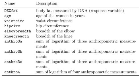
A plot of the coefficient paths, similar to the ones commonly known from the LARS algorithm (Efron et al 2004), can be easily produced by usingplot()on the glmboostobject (see Figure 1):
R> plot(glm2b, off2int = TRUE) ## default plot, offset added to intercept R> ## now change ylim to the range of the coefficients without intercept (zoom-in) R> plot(glm2b, ylim = range(coef(glm2b, which = preds)))
0 20 40 60 80 100 −60 −40 −20 0 20
Number of boosting iterations
Coefficients (Intercept) elbowbreadth age waistcirc hipcirc anthro3c kneebreadth anthro3a anthro3b 0 20 40 60 80 100 0 1 2 3
Number of boosting iterations
Coefficients elbowbreadth age waistcirc hipcirc anthro3c kneebreadth anthro3a anthro3b
Figure 1: Coefficents paths with the body fat data, default plot (left) and with an adjusted y-scale (right).
3A third alternative is given by the matrix interface forglmboost()where one can directly use the design matrix as an argument.
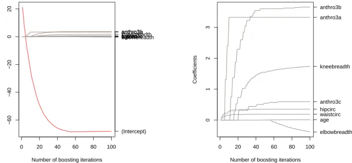
Centering of Linear Base-learners Without Intercept
For linear base-learners that are specified without intercept,4it is of great importance to center the covariates before fitting the model. Without centering of the covariates, linear effects that result from base-learners without intercept are forced through the origin (with no data lying there). Hence, the convergence will be very slow or the algorithm will not converge to the “correct” solution even in very simple cases. As an example, consider one normally distributed predictorx= (x1, . . . , xn)>, and a model
y=βx+ε,
withβ= 1 andε∼ N(0,0.32). Usually, a model without intercept could be fitted to estimateβ. However, if we apply boosting with the L2 loss the negative gradient in the first boosting step is, by default, the centered response, i.e., u[1] = y
−1/nPni=1yi. For other loss functions the negative gradient in the first boosting
iteration is not exactly the mean-centered response. Yet, the negative gradient in the first step is always “centered” around zero. In this situation, the application of a base-learner without intercept (i.e., a simple linear model without intercept) is not sufficient anymore to recover the effectβ (see Figure 2(a)). The true effect is completely missed. To solve this problem, it is sufficient to use a centered predictor x. Then, the center of the data is shifted to the origin (see Figure 2(b)) and the model without intercept goes through the origin as well. 0 2 4 6 −2 −1 0 1 2 x negativ e gr adient in step m = 1 origin center of data base−learner
(a) Without Centering
−4 −2 0 2 −2 −1 0 1 2 x (centered) negativ e gr adient in step m = 1 (b) With Centering
Figure 2: L2Boosting in the first boosting step, i.e., with centered response variable as outcome. A base-learner without intercept misses the true effect completely ifxis not centered (left) and is able to capture the true structure ifxis centered (right).
Centering the predictors does not change the estimated effects of the predictors. Yet, the intercept needs to be corrected as can be seen from the following example. Consider two predictors and estimate a model with centered predictors, i.e,
ˆ y= ˆβ0+ ˆβ1(x1−x1) + ˆ¯ β2(x2−x2)¯ ⇔ ˆ y= ( ˆβ0−β1ˆ x1¯ −β2ˆ x2)¯ | {z } = ˆβ∗ 0 + ˆβ1x1+ ˆβ2x2.
Hence, the intercept from a model without centering of the covariates equals ˆβ∗
0 = ˆβ0−Pjβˆjx¯j, where ˆβ0is
the intercept estimated from a model with centered predictors.
3.2 Fitting Generalized Additive Models:
gamboost
Besides an interface to fit linear models,mboostoffers a very flexible and powerful function to fit structured additive models. This function,gamboost()can be used to fit linear models or (non-linear) additive models via component-wise boosting. The user additionally needs to state which variable should enter the model in
4If the fitting functionglmboost() is used the base-learners never contain an intercept. Furthermore, linear base-learners
which fashion, e.g. as a linear effect or as a smooth effect. In general, however, the interface of gamboost()
is very similar toglmboost().
gamboost(formula, data = list(), ...)
Again, the function requires a formula to specify the model. Furthermore, a data set needs to be specified as for linear models. Additional arguments that are passed to mboost_fit()5 include weights, controland
family. These arguments can be used in the same way as described forglmboost()above.
3.2.1 Base-learners
The structural assumption of the model, i.e., the types of effects that are to be used, can be specified in terms of base-learners. Each base-learner results in a related type of effect. An overview of available base-learners is given in the following paragraphs. An example of how these base-learners can then be combined to formulate the model is given afterwards.
The base-learners should be defined such that the degrees of freedom of the single base-learner are small enough to prevent overshooting. Typically one uses, for example, 4 degrees of freedom (the default for many base-learners) or less. Despite the small initial degrees of freedom, the final estimate that results from this base-learner can adopt higher order degrees of freedom due to the iterative nature of the algorithm. If the base-learner is chosen multiple times, it overall adapts to an appropriate degree of flexibility and smoothness. Linear and Categorical Effects
The bols() function6 allows the definition of (penalized) ordinary least squares base-learners. Examples
of base-learners of this type include (a) linear effects, (b) categorical effects, (c) linear effects for groups of variablesx= (x1, x2, . . . , xp)>, (d) ridge-penalized effects for (b) and (c), (e) varying coefficient terms (i.e.,
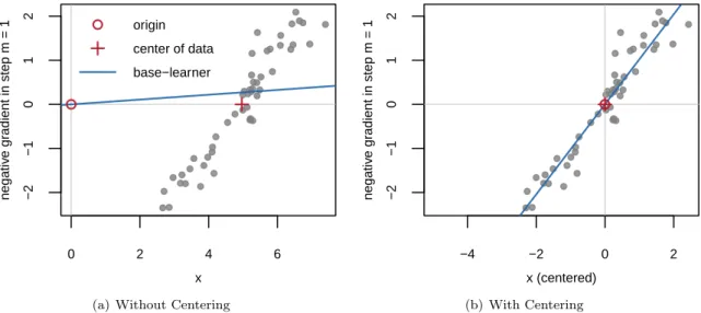
interactions), etc. If a penalized base-learner is specified, a special penalty based on the differences of the effects of adjacent categories is automatically used for ordinal variables (x <- as.ordered(x)) instead of the ridge penalty (Hofner et al 2011a). Figure 3 shows two effect estimates that result frombols()base-learners, a simple linear effect and an effect estimate for a factor variable. The call to an ordinary penalized least squares base-learner looks as follows:
bols(..., by = NULL, intercept = TRUE, df = NULL, lambda = 0)
The variables that correspond to the base-learner are specified in the ‘...’ argument, separated by commas. If multiple variables are specified, they are treated asone group. A linear model is fitted for all given variables together and they are either all updated or not at all. An additional variable that defines varying coefficients can optionally be given in thebyargument. The logical variableinterceptdetermines whether an intercept is added to the design matrix (intercept = TRUE, the default). Ifintercept = FALSE, continuous covariates should be (mean-) centered as discussed above. This must be done ‘by hand’ in advance of fitting the model. The impact of the penalty in case of penalized OLS base-learners can be determined either via the degrees of freedomdfor the penalty parameter lambda. If degrees of freedom are specified, the penalty parameter
lambdais computed from df7. Note that per default unpenalized linear models are used. Two definitions
of degrees of freedom are implemented inmboost: The first uses the trace of the hat-matrix (trace(S)) as degrees of freedom, while the second definition uses trace(2S − S>S). The latter definition is tailored to the comparison of models based on residual sums of squares and hence is better suitable in the boosting context (see Hofner et al 2011a, for details).
Table 2 shows some calls to bols()and gives the resulting type of effect. To gain more information on a specific base-learner it is possible to inspect the base-learners inmboostusing the functionextract()on a base-learner or a boosting model. With the function one can extract, for example, the design matrices, the penalty matrices and many more characteristics of the base-learners. For a detailed instruction on how to use the function see the manual forextract()and especially the examples therein.
Smooth Effects
Thebbs() base-learner8 allows the definition of smooth effects based on B-splines with difference penalty
(i.e., P-splines, cf. Eilers and Marx 1996). A wide class of effects can be specified using P-splines. Examples
5gamboost()also callsmboost_fit()for the actual boosting algorithm. 6the name refers toordinaryleastsquares base-learner
7If dfis specified inbols(),lambdais always ignored. 8the name refers to B-splines with penalty, hence the second b
−2 −1 0 1 2 3 4 −1.0 −0.5 0.0 0.5 1.0 1.5 2.0 x1 f ( x1 ) ● ●●●●● ● ●●●●●● ● ●● ●● ●●● ●●●● ●●●●●● ● ●●●●● ●● ●●●●●●●●●●●●●●●●●●●●●●●●●●●●● ● ●●●●●● ● ●●●● ●●●● ●● ●●●●●●●● ● ● ● ● ● ● ● true effect model −1 0 1 2 3 x2 f ( x2 ) x2 (1) x2 (2) x2 (3) x2 (4) ● ● ● ● ● ● ● ● ● ● ● ● ● true effect model
Figure 3: Examples for linear and categorical effects estimated using bols(): Linear effect (left; f(x1) = 0.5x1) and categorical effect (right;f(x2) = 0x(1)2 −1x
(2) 2 + 0.5x (3) 2 + 3x (4) 2 )
Table 2: Some examples of effects that result from bols()
Call Type of Effect
bols(x) linear effect: x>βwithx>= (1, x)
bols(x, intercept = FALSE) linear effect without intercept: β·x
bols(z) OLS fit with factor z (i.e., linear effect after dummy
coding)
bols(z, df = 1) ridge-penalized OLS fit with one degree of freedom and
factorz; Ifz is an ordered factor a difference penalty is used instead of the ridge penalty.
bols(x1, x2, x3) one base-learner for three variables (group-wise
selec-tion):
x>βwithx> = (1, x1, x2, x3)
bols(x, by = z) interaction: x>β·z(with continuous variablez). Ifz
is a factor, a separate effect is estimated for each factor level; Note that in this case, the main effect needs to be specified additionally viabols(x).
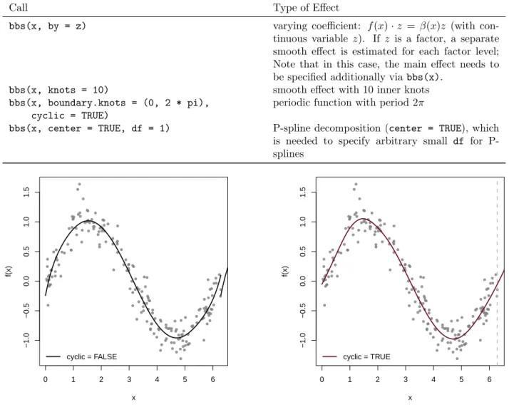
include (a) smooth effects, (b) bivariate smooth effects (e.g., spatial effects), (c) varying coefficient terms, (d) cyclic effects (= periodic effects) and many more. Two examples of smooth function estimates fitted using a
bbs()base-learner are given in Figure 4. The call to a P-spline base-learner is as follows:
bbs(..., by = NULL, knots = 20, boundary.knots = NULL, degree = 3, differences = 2, df = 4, lambda = NULL, center = FALSE, cyclic = FALSE)
As for all base-learners, the variables that correspond to the base-learner can be specified in the ‘...’ argument. Usually, only one variable is specified here for smooth effects, and at maximum two variables are allowed forbbs(). Varying coefficient terms f(x)·z can be specified using bbs(x, by = z). In this case, xis called the effect modifier of the effect ofz. The knotsargument can be used to specify the number of equidistant knots, or the positions of the interior knots. In case of two variables, one can also use a named list to specify the number or the position of the interior knots for each of the variables separately. For an example of the usage of a named list see Section 3.2.2. The location of boundary knots (default: range of the data) can be specified usingboundary.knots. Usually, no user-input is required here. The only exception is given for cyclic splines (see below). The degree of the B-spline bases (degree) and the order of the difference penalty (differences;∈ {0,1,2,3}) can be used to specify further characteristics of the spline estimate. The latter parameter specifies the type of boundary effect. Fordifferences = 2, for example, deviations from
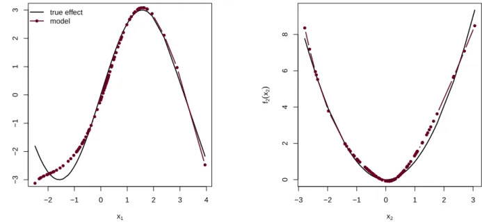
−2 −1 0 1 2 3 4 −3 −2 −1 0 1 2 3 x1 f1 ( x1 ) ● ●●●●● ●●●●●●●● ●● ●● ● ●●●●●● ●●●●● ● ● ●●● ● ● ● ● ●●● ● ●● ●●● ● ●● ● ● ●●●●●●●●●●● ● ● ● ● ● ●● ● ● ● ● ● ●●● ● ● ● ●● ●● ●●●●●●●●●● ● ● ● ● ● true effect model −3 −2 −1 0 1 2 3 0 2 4 6 8 x2 f2 ( x2 ) ● ● ● ● ● ● ● ● ● ● ●● ●● ●●● ● ●●●●●●●●●●●●●● ●●●●●●●●● ● ●●●●●●●●●●●●●●●●●●●●●● ●●●●●●●●● ● ●●●● ● ●●●●●●●●● ● ● ●● ●● ● ● ● ● ● ●
Figure 4: Examples for smooth effects estimated using bbs(). True effect f1(x1) = 3·sin(x1) (left) and f2(x2) =x2
2(right).
a linear function are penalized. In the case of first order differences, deviations from a constant are subject to penalization. The smoothness of the base-learner can be specified using degrees of freedom (df) or the smoothing parameter (lambda)9.
An issue in the context of P-splines is that one cannot make the degrees of freedom arbitrary small. A polynomial of order differences - 1 always remains unpenalized (i.e., the so-called null space). As we usually apply second order differences, a linear effect (with intercept) remains unpenalized and thus df ≥2 for all smoothing parameters. A solution is given by a P-spline decomposition (see Kneib et al 2009; Hofner et al 2011a). The smooth effectf(x) is decomposed in the unpenalized polynomial and a smooth deviation from this polynomial. For differences of order 2 (= default), we thus get:
f(x) = β0+β1x | {z } unpenalized polynomial + fcentered(x) | {z } smooth deviation (3)
The unpenalized polynomial can then be specified using bols(x, intercept = FALSE) and the smooth deviation is obtained bybbs(x, center = TRUE). Additionally, it is usually advised to specify an explicit base-learner for the intercept (see Section 3.2.2).
A special P-spline base-learner is obtained if cyclic = TRUE. In this case, the fitted values are forced to coincide at the boundary knots and the function estimate is smoothly joined (see Figure 5). This is especially interesting for time-series or longitudinal data were smooth, periodic functions should be modeled. In this case it is of great importance, that the boundary knots are properly specified to match the points were the function should be joined (due to subject matter knowledge).
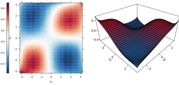
An non-exhaustive overview of some usage scenarios forbbs()base-learners is given in Table 3. Smooth Surface Estimation
An extension of P-splines to two dimensions is given by bivariate P-splines. They allow to fit spatial effects and smooth interaction surfaces. An example of a two dimensional function estimate is given in Figure 6. The effects can be obtained from a call to
bspatial(..., df = 6)
To specify two dimensional smooth effects, the ‘...’ argument requires two variables, i.e., a call such as
bspatial(x, y). Note that bspatial() is just a wrapper to bbs() with redefined degrees of freedom10.
Thus, all arguments frombbs()exist and can be used forbspatial(). An example is given in Section 3.2.2.
9If lambdais specified inbbs(),dfis always ignored. 10Note thatdf = 4was changed todf = 6inmboost2.1-0.
Table 3: Some examples of effects that result from bbs()
Call Type of Effect
bbs(x, by = z) varying coefficient: f(x)·z = β(x)z (with
con-tinuous variable z). If z is a factor, a separate smooth effect is estimated for each factor level; Note that in this case, the main effect needs to be specified additionally via bbs(x).
bbs(x, knots = 10) smooth effect with 10 inner knots
bbs(x, boundary.knots = (0, 2 * pi), cyclic = TRUE)
periodic function with period 2π
bbs(x, center = TRUE, df = 1) P-spline decomposition (center = TRUE), which
is needed to specify arbitrary small df for P-splines 0 1 2 3 4 5 6 −1.0 −0.5 0.0 0.5 1.0 1.5 x f(x) cyclic = FALSE 0 1 2 3 4 5 6 −1.0 −0.5 0.0 0.5 1.0 1.5 x f(x) cyclic = TRUE
Figure 5: Example for cyclic splines. The unconstrained effect in the left figure is fitted usingbbs(x, knots = 12), the cyclic effect in the right is estimates usingbbs(x, cyclic = TRUE, knots = 12,
bound-ary.knots = c(0, 2*pi)). True effect: f(x) = sin(x)..
Random Effects
To specify random intercept or random slope terms inmboost, one can use a random effects base-learner. Random effects are modeled as ridge-penalized group-specific effects. One can show that these coincide with standard random effects. The ridge penalty parameter is then simply the ratio of the error varianceσ2 and the random effects variance τ2. Hence, the penalty parameter is inversely linked toτ2 (and the degrees of freedom are directly linked toτ2). As for all base-learners, we initially specify a small value for the degrees of freedom, i.e., we set a small random effects variance (relative to the residual variance). By repeatedly selecting the base-learner, the boosting algorithm can then adapt to the “true” random effects variance. For more details see Kneib et al (2009, Web Appendix). We can specify random effects base-learners with a call to
brandom(..., df = 4)
As brandom() is just a wrapper of bols() with redefined degrees of freedom, one can use all arguments
that are available for bols(). To specify a random intercept for a group variable, say id, we simply call
brandom(id)(and could additionally specify theinitialerror variance viadforlambda). To specify a random
slope for another variable, saytime, within the groups ofid, one can usebrandom(id, by = time), i.e., the first argument determines the grouping (as for the random intercept) and thebyargument then determines the variable for which the effect is allowed to vary between the groups. In the notation of nlme (Pinheiro et al 2012) andlme4(Bates et al 2011) the random intercept would be specified as(1 | id)and the random
x1 x2 −3 −2 −1 0 1 2 3 −3 −2 −1 0 1 2 3 −0.4 −0.2 0.0 0.2 0.4 0.6 x1 −2 0 2 x2 −2 0 2 −0.5 0.0 0.5
Figure 6: Example for interaction surface fitted usingbspatial(). Two displays of the same function estimate are presented (levelplot: left; perspective plot: right). True function: f(x1, x2) = sin(x1)·sin(x2).
slope would be specified as(time - 1 | id), i.e., a random slope without random intercept term. Additional Base-learners in a Nutshell
Tree-based base-learner (per default stumps) can be included in the model using the btree()base-learner (Hothorn et al 2006, 2010). Note that this is the only base-learner which is not fitted using penalized least squares. Radial basis functions (e.g., for spatial effects) can be specified using the base-learnerbrad(). Details on this base-learner are given in (Hofner 2011). Monotonic effects of continuous or ordered categorical variables can be estimated using thebmono()base-learner which can also estimate convex or concave effects. Details on monotonic effect estimation and examples of the estimation of boosting models with monotonic effects are given in Hofner et al (2011b) in the context of species distribution models. The base-learner
bmrf()implements Markov random fields, which can be used for the estimation of spatial effects of regions
(Sobotka and Kneib 2010; Mayr et al 2012a). With the base-learnerbuser(), one can specify arbitrary base-learners with quadratic penalty. This base-learner is dedicated to advanced users only. Additionally, special concatenation operators for expert users exist inmboost that all combine two or more base-learners to a single base-learner: %+%additively joins two or more arbitrary base-learners to be treated as one group, %X%
defines a tensor product of two base-learners and%O%implements the Kronecker product of two base-learners. In all cases the degrees of freedom increase compared to the degrees of freedom of the single base-learners (additively in the first, and multiplicatively in the second and third case). For more details on any of these base-learners and for some usage examples see the manual.
3.2.2 Building a Model – or: How to Combine Different Base-learners
Base-learners can be combined in a simple manner to form a model. They are combined in the formula as a sum of base-learners to specify the desired model. We will show this using a simple toy example:
R> m1 <- gamboost(y ~ bols(x1) + bbs(x2) + bspatial(s1, s2) + brandom(id), + data = example)
In this case, a linear effect forx1, a smooth (P-spline) effect forx2, a spatial effect fors1ands2are specified together with a random intercept forid. This model could be further refined and expanded as shown in the following example:
R> m2 <- gamboost(y ~ bols(int, intercept = FALSE) + + bols(x1, intercept = FALSE) + + bols(x2, intercept = FALSE) + + bbs(x2, center = TRUE, df = 1) +
+ brandom(id) + brandom(id, by = x1), + data = example)
Now, with example$int = rep(1, length(y)), we specify a separate intercept in the model. In the first formula (m1), the intercept was implicitly included in the base-learners. Now we allow the boosting algorithm to explicitly choose and update solely the intercept. Note that therefor we need to remove the implicit intercept from the base-learner forint(intercept = FALSE) as otherwise we would get a linear base-learner with two intercepts which has no unique solution. We can now also remove the intercept from the base-learner of x1. This leads to a base-learner of the form x1β1. For the smooth effect of x2 we now use the decomposition (3). Hence, we specify the unpenalized part as a linear effect without intercept (the intercept is already specified in the formula) and the smooth deviation from the linear effect (with one degree of freedom). Now the boosting algorithm can choose howx2should enter the model: (i) not at all, (ii) as a linear effect, (iii) as a smooth effect centered around zero, or (iv) as the combination of the linear effect and the smooth deviation. In the latter case we essentially get the same result as frombbs(x2). The spatial base-learner in the second formula (m2) explicitly specifies the numbers of knots in the direction ofs1(10 inner knots) ands2
(20 inner knots). This is achieved by a named list where the names correspond to the names of the variables. In total we get 10·20 = 200 inner knots. Usually, one specifies equal numbers of knots in both directions, which requires no named lists. Instead one can simply specify, e.g.,knots = 10, which results in 10 inner knots per direction (i.e., 100 inner knots in total). Note that, as for the smooth, univariate base-learner of
x2one could also specify a decomposition for the spatial base-learner:
bols(int, intercept = FALSE) +
bols(s1, intercept = FALSE) + bols(s2, intercept = FALSE) + bols(s1 * s2, intercept = FALSE) +
bspatial(s1, s2, center = TRUE, df = 1)
Finally, we added a random slope forx1(in the groups of id) tom2. Note that the groups are the argument of the base-learner and the slope variable is specified via thebyargument.
Case Study (ctd.): Prediction of Body Fat
Until now, we only included linear effects in the prediction formula for body fat of women. It might be of interest to evaluate if there exists also a non-linear relationship between some of the predictors and the DXA measurement of body fat. To investigate this issue, we fit a model with the same predictors as in Garcia et al (2005) but without assuming linearity of the effects. We applygamboost() with the P-spline base-learner
bbs()to incorporate smooth effects.
R> ## now an additive model with the same variables as lm1
R> gam1 <- gamboost(DEXfat ~ bbs(hipcirc) + bbs(kneebreadth) + bbs(anthro3a), R> data = bodyfat)
Usingplot()on agamboostobject delivers automatically the partial effects of the different base-learners:
R> par(mfrow = c(1,3)) ## 3 plots in one device R> plot(gam1) ## get the partial effects
From the resulting Figure 7, it seems as if in the center of the predictor-grid (where most of the observations lie), the relationship between these three anthropometric measurements and the body fat is quite close to a linear function. However, at least for hipcirc, it seems that there are indications of the existence of a non-linear relationship for higher values of the predictor.
Alternatively, one could apply decomposition (3) for each of the 3 base-learners, as described in Sec-tion 3.2.2, to distinguish between modeling alternatives. In this case, we would have a more rigorous treat-ment of the decision between (purely) linear and non-linear effects if we stop the algorithm at an appropriate iterationmstop.
3.3 Early Stopping to Prevent Overfitting
As already discussed in Section 2, the major tuning parameter of boosting is the number of iterationsmstop. To prevent overfitting it is important that the optimal stopping iteration is carefully chosen. Various possibilities to determine the stopping iteration exist. One can use information criteria such as AIC11to find the optimal model. However, this is usually not recommended as AIC based stopping tends to overshoot the optimalmstop
●● ● ●● ● ●●● ●●● ●●●● ●● ● ● ● ● ● ●●●●● ●●● ●●●● ● ●● ●● ● ● ● ●●● ● ● ● ● ●● ● ● ● ● ●●●● ● ●●●●●●● ● ● ● 90 100 110 120 130 −10 −5 0 5 10 hipcirc fpa rt ia l ● ●●●●●●●●●●●●●●●●●●●●●●●●●●●●●●●●●●●●●●● ● ● ●●●●●●●●●●●●● ● ● ● ● ● ● ● ●●●● ●● ● ● ● 8 9 10 11 −10 −5 0 5 10 kneebreadth fpa rt ia l ● ● ● ●●● ●● ●●● ●● ●●● ● ●● ● ●●●● ●●● ●● ●●●●●●●● ●●●●●●● ●●●●●●●●●●● ● ● ●● ●● ● ● ● ●● ●● ● ● ● 2.5 3.0 3.5 4.0 4.5 −10 −5 0 5 10 anthro3a fpa rt ia l
Figure 7: Partial effects of three anthropometric measurements on the body fat of women.
dramatically (see Hastie 2007; Mayr et al 2012b). Instead, it is advised to use cross-validated estimates of the empirical risk to choose an appropriate number of boosting iterations. This approach aims at optimizing the prognosis on new data. Inmboost infrastructure exists to compute bootstrap estimates, k-fold cross-validation estimates and sub-sampling estimates. The main function to determine the cross-validated risk is
cvrisk(object, folds = cv(model.weights(object)),
papply = if (require("multicore")) mclapply else lapply)
In the simplest case, the user only needs to specify the fitted boosting model as object. If one wants to change the default cross-validation method (25-fold bootstrap) the user can specify a weight matrix that determines the cross-validation samples via thefoldsargument. This can be done either by hand or using the convenience functioncv()(see below). Finally, the user can specify a function of thelapply“type” to
papply. Per default this is eithermclapplyfor parallel computing if package multicore(Urbanek 2011) is
available, or the code is run sequentially usinglapply. Alternatively, the user can apply other parallelization methods such asclusterApplyLB(packagesnowTierney et al 2011) with some further effort for the setup
(see?cvrisk).
The easiest way to set up a variety of weight matrices for cross-validation is the function
cv(weights, type = c("bootstrap", "kfold", "subsampling"), B = ifelse(type == "kfold", 10, 25))
One simply specifies the weights of the originally fitted model (e.g. using the function model.weights()
on the model) and thetype of cross-validation. This can be either"bootstrap" (default),"kfold"(k-fold cross-validation) or"subsampling"12. The number of cross-validation replicates, per default, is chosen to be 10 for k-fold cross-validation and 25 otherwise. However, one can simply specify another number of replicates using the argumentB.
To extract the appropriate number of boosting iterations from an object returned by cvrisk()(orAIC()) one can use the extractor functionmstop(). Once an appropriate number of iterations is found, we finally need to stop the model at this number of iterations. To increase or reduce the number of boosting steps for the modelmod, one can use the indexing / subsetting operator directly on the model:
mod[i]
whereiis the number of boosting iterations. Attention, the subset operator differs in this context from the standardRbehavior as itdirectly changes the model mod. Hence, there is no need to savemodunder a new name. This helps to reduce the memory footprint. Be aware that even if you call something like
12the percentage of observations to be included in the learning samples for subsampling can be specified using a further argument
newmod <- mod[10]
you will change the boosting iteration ofmod! Even more, if you now changemstopfornewmod, the modelmod
is also changed (and vice versa)! This said, the good news is that nothing gets lost. If we reduce the model to a lower value ofmstop, the additional boosting steps are kept internally in the model object. Consider as an example the following scenario:
• We fit an initial modelmodwithmstop = 100.
• We callmod[10], which setsmstop = 10.
• We now increasemstopto 40 with a call to mod[40].
This now requiresno re-computation of the model as internally everything was kept in storage. Again the warning, if we now extract anything from the model, such ascoef(mod), we get the characteristics of the model with 40 iterations, i.e., here the coefficient estimates from the 40th boosting iteration.
Case Study (ctd.): Prediction of Body Fat
Until now, we used the default settings ofboost_control() withmstop = 100for all boosted models. Now we want to optimize this tuning parameter with respect to predictive accuracy, in order get the best prediction for body fat. Note that tuningmstopalso leads to models including only the most informative predictors as variable selection is carried out simultaneously. We therefore first fit a model with all available predictors and then tunemstopby 25-fold bootstrapping. Using thebaselearnerargument ingamboost(), we specify the default base-learner which is used for each variable in the formula for which no base-learner is explicitly specified.
R> ## every predictor enters the model via a bbs() base-learner (i.e., as smooth effect) R> gam2 <- gamboost(DEXfat ~ ., baselearner = "bbs", data = bodyfat,
+ control = boost_control(trace = TRUE))
[ 1] ... -- risk: 483.4287
[ 48] ... -- risk: 412.9833
[ 95] ....
Final risk: 406.6785
R> set.seed(123) ## set seed to make results reproducible
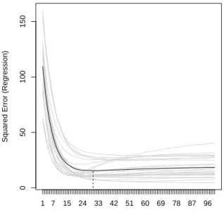
R> cvm <- cvrisk(gam2) ## default method is 25-fold bootstrap cross-validation R> ## if package ’multicore’ is not available this will trigger a warning
R> cvm
Cross-validated Squared Error (Regression)
gamboost(formula = DEXfat ~ ., data = bodyfat, baselearner = "bbs")
1 2 3 4 5 6 7
109.44090 93.77936 80.39199 69.39746 60.03652 52.63142 45.98735
(...)
97 98 99 100
18.42903 18.44325 18.47198 18.50329
Optimal number of boosting iterations: 30
R> plot(cvm) ## get the paths
The plot displays the predictive risk on the 25 bootstrap samples formstop= 1, ...,100 (see Figure 8). The optimal stopping iteration is the one minimizing the average risk over all 25 samples. We can extract this iteration via
R> mstop(cvm) ## extract the optimal mstop
Number of boosting iterations
Squared Error (Regression)
1 7 15 24 33 42 51 60 69 78 87 96
0
50
100
150
Figure 8: Cross-validated predictive risk with 25-fold bootstrapping.
R> gam2[ mstop(cvm) ] ## set the model automatically to the optimal mstop
We have now reduced the model of the objectgam2to the one with only 30 boosting iterations, without further assignment. However, as pointed out above, the other iterations are not lost. To check which variables are now included in the additive predictor we again use the functioncoef():
R> names(coef(gam2)) ## displays the selected base-learners at iteration 30
[1] "bbs(waistcirc, df = dfbase)" "bbs(hipcirc, df = dfbase)"
[3] "bbs(kneebreadth, df = dfbase)" "bbs(anthro3a, df = dfbase)"
[5] "bbs(anthro3b, df = dfbase)" "bbs(anthro3c, df = dfbase)"
R> ## To see that nothing got lost we now increase mstop to 1000: R> gam2[1000]
[ 101] ... -- risk: 370.0461 [ 148] ... -- risk: 344.4602 ( ... )
Although we earlier had reduced to iteration 30, the fitting algorithm started at iteration 101. The iterations 31-100 are not re-computed.
R> names(coef(gam2)) ## displays the selected base-learners, now at iteration 1000
[1] "bbs(age, df = dfbase)" "bbs(waistcirc, df = dfbase)"
[3] "bbs(hipcirc, df = dfbase)" "bbs(elbowbreadth, df = dfbase)"
[5] "bbs(kneebreadth, df = dfbase)" "bbs(anthro3a, df = dfbase)"
[7] "bbs(anthro3b, df = dfbase)" "bbs(anthro3c, df = dfbase)"
[9] "bbs(anthro4, df = dfbase)"
The stopping iteration mstop is the main tuning parameter for boosting and controls the complexity of the model. Larger values for mstop lead to larger and more complex models, while for smaller values the complexity of the model is generally reduced. In our example the final model at iteration 1000 includes all available variables as predictors for body fat, while the model at the optimal iteration 30 included only five predictors. Optimizing the stopping iteration usually leads to selecting the most influential predictors.
3.4 Specifying the Fitting Problem: The
family
The list of implemented families inmboostis diverse and wide-ranging. At the time of writing this paper, the user has access to sixteen different families. A family (most importantly) implements the loss functionρ and the corresponding negative gradient. A careful specification of the loss function leads to the estimation
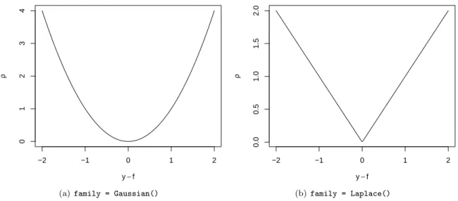
−2 −1 0 1 2 0 1 2 3 4 y−f ρ
(a)family = Gaussian()
−2 −1 0 1 2 0.0 0.5 1.0 1.5 2.0 y−f ρ (b)family = Laplace()
Figure 9: The loss function allows flexible specification of the link between the response and the covariates. The figure on the left hand side illustrates the L2 loss (the default inmboost), the figure on the right hand side shows the L1loss function.
of any desired characteristic of the conditional distribution of the response. This coupled with the large number of base learners guarantees a rich set of models that can be addressed by boosting. We can specify the connection between the response and the covariates in a fairly modular nature such as
ξ(y|x) = ˆf1+· · ·+ ˆfP (4)
having on the right hand side any desired combination of base learners. On the left hand side, ξ(.) de-scribessomecharacteristic of the conditional distribution specified by thefamilyargument. In the following subsections we discuss major aspects relating to the choice of the family.
3.4.1 Families for Continuous Response
Until now the focus was on the conditional mean of a continuous response which is the default setting:family
= Gaussian(). In this case, our assumption is thatY|xis normally distributed and the loss function is the
negative Gaussian log-likelihood which is equivalent to the L2loss ρ(y, f) =1
2(y−f)
2 (5)
(see Figure 9(a)). A plainGaussian()call in the console returns its definition
R> Gaussian()
Squared Error (Regression) Loss function: (y - f)^2
The corresponding negative gradient is simply (y−f) whose definition can be displayed on the screen via
R> slot(Gaussian(),"ngradient")
function (y, f, w = 1) y - f
If we are interested in the median of the conditional distribution, theLaplace()family is the right choice. It implements a distribution free, median regression approach especially useful for long-tailed error distributions. In this case, we use the L1 loss defined as
ρ(y, f) =|y−f| (6)
and shown in Figure 9(b). Note that the L1 loss is not differentiable aty=f and the value of the negative gradient at such points is fixed at zero.
−2 −1 0 1 2 0.0 0.5 1.0 1.5 2.0 y−f ρ δ 0.2 0.5 1 2 10
(a)family = Huber()
−2 −1 0 1 2 0.0 0.5 1.0 1.5 2.0 y−f ρ τ 0.5 0.6 0.7 0.8 0.9 (b)family = QuantReg()
Figure 10: The Huber loss function on the left hand side is useful when robustness is a concern. Inmboost
it adaptively changes the limit for L1 penalization of outliers whend = NULL(the default). The figure on right hand side illustrates several examples of the check function loss with different quantiles (tau = 0.5is the default).
A compromise between the L1 and the L2 loss is the Huber loss function shown in Figure 10(a). It is defined as ρ(y, f;δ) = ( (y−f)2/2 if |y−f| ≤δ, δ(|y−f| −δ/2) if|y−f|> δ (7) where the parameter δ limits the outliers which are subject to absolute error loss. The Huber loss can be seen as a robust alternative to the L2 loss. The user can either specify δ subjectively, e.g. Huber(d = 2), or leave it adaptively chosen by the boosting algorithm (the default behaviour). An adaptive specification ofδ, proposed by Friedman (2001), means that each boosting step produces a newδ[m] matching the actual median of the absolute values of the residuals, i.e.
δ[m]= medianyi−fˆ[m−1](xi)
, i= 1, . . . , n. (8) Another alternative for settings with continuous response is modeling conditional quantiles through quantile regression (Koenker 2005) – implemented inmboostwith theQuantReg() family (Fenske et al 2011). The main advantage of quantile regression is (beyond its robustness toward outliers) that it does not rely on any distributional assumptions on the response or the error terms. The appropriate loss function here is the check-function shown in Figure 10(b). For the special case of the 0.5 quantile bothQuantReg(0.5)and
Laplace()will lead to median regression. A detailed description of the loss function of quantile regression
is given in the Appendix.
Case Study (ctd.): Prediction of Body Fat
We reproduce the model of the original publication (Garcia et al 2005), but instead of modeling the mean we focus on the median:
R> ## Same model as glm1 but now with QuantReg() family
R> glm3 <- glmboost(DEXfat ~ hipcirc + kneebreadth + anthro3a, data = bodyfat,
+ family = QuantReg(tau = 0.5), control = boost_control(mstop = 500)) R> coef(glm3, off2int = TRUE)
(Intercept) hipcirc kneebreadth anthro3a
-63.5164304 0.5331394 0.7699975 7.8350858
Comparing the results to those of model glm1 shows that hipcirc and anthro3a have almost the same influence on the mean as on the median, yet, the magnitude of the effect of kneebreadth is considerably smaller inglm3. One should note thatmstopgenerally needs to be larger for quantile regression, as the single updates are smaller than in the mean regression case. For a discussion see the Appendix.
−2 −1 0 1 2 0 2 4 6 y ~f ρ loss Binomial AdaExp
Figure 11: TheBinomialand theAdaExpfamilies as functions of the marginal values ˜yf. Since ˜y∈ {−1,1}, a positive product between ˜y and half the estimated log-odds ratio f means correct categorical discrimination.
3.4.2 Families for Binary Response
Analogously to Gaussian regression, the probability parameter of a binary response can be estimated by minimizing the negative binomial log-likelihood
ρ(y, f) =−y log π(f)+ (1−y) log 1−π(f)
= log(1 + exp(−2 ˜yf)) (9)
where ˜y = 2y−1 and π(f) = P(Y = 1|x). For reasons of computational efficiency the binary response y ∈ {0,1} is converted into ˜y = 2y −1 where ˜y ∈ {−1,1}. In equation (9) ˜yf are the so-called margin values (depicted in Figure 11) which are, roughly speaking, the equivalent of the continuous residualsy−f for the binomial case. This internal re-coding13means that the negative binomial log-likelihood loss (family
= Binomial()) and the exponential loss (family = AdaExp()) coincide in their population minimizer (see
B¨uhlmann and Hothorn 2007, Section 3).
Note that the transformation ˜y = 2y−1 changes the interpretation of the effect estimates because now we get the half of the log-odd ratio. One implication is that thecoef() output is half the estimations that result fromglm(). This means that the user has to double the coefficientsmanually in order to get the final standard estimates of a logistic regression model.
However, mboostautomatically doubles the logits prior to the reverse probability transformation. This means that calling predict(fit, newdata, type = "response") produces the final probability estima-tions. In addition to the logit model, the user can also estimate probit models usingfamily = Binomial(link = "probit").
Alternatively one can also use the exponential loss function ρ(y, f) = exp(−yf) (˜ family = AdaExp()). This essentially leads to the famous AdaBoost algorithm by Freund and Schapire (1996). As can be seen in Figure 11, this loss function is similar toBinomial().
3.4.3 Families for Count Data and Censored Response
Inmboost, currently two families handle data with count response. The Poisson() family uses the neg-ative Poisson log-likelihood with the natural link function log(µ) =η. Alternatively, the negative binomial distribution can be used to model overdispersed data. The negative log-likelihood density of this distribu-tion is implemented inNBinomial(nuirange = c(0, 100))where the parameternuirange(accounting for overdispersion) is optimized additionally within each boosting iterationm. One simply minimizes the em-pirical riskRover the overdispersion parameter given the current boosting estimate ˆf[m] after step 4 of the component-wise gradient boosting algorithm. A thorough introduction and the detailed algorithm is given by Schmid et al (2010).
Survival models can also be considered in mboost: CoxPH(), Weibull(), Loglog() and Lognormal()
all implement families for censored data. CoxPH() implements the Cox proportional hazards model while the other three families specify accelerated failure time (AFT) models (see Schmid and Hothorn 2008b, for further details).
3.4.4 Further Families
Additionally to the families discussed above,mboostimplements some further families: AUC()can be used to optimize the area under the ROC curve, GammaReg() implements the negative Gamma log-likelihood with logarithmic link function,ExpectReg()implements expectile regression (Sobotka and Kneib 2010) and
PropOdds()leads to proportional odds models for ordinal outcome variables (Schmid et al 2011).
Despite the wide range of available families, users might wish to implement new loss functions. One only needs a loss function and the corresponding negative gradientδρ(y, f)/ δf, which both are independent of the base-learners. Using the constructor functionFamily(), one can then easily define new families and thus new estimation problems as we show in the Appendix.
4 Summary
The R-packagemboostoffers an easy entry into the world of boosting. It implements a model-based boosting approach that results in interpretable structured additive models of the same form most researchers will feel familiar with. The interfaces of fitting functions are quite similar to standard implementations likelm() or
glm()and are hence relatively easy to use. However, the fitting algorithms of mboostadditionally offer a
high flexibility when it comes to the effect type of potential predictors and the type of risk function to be optimized. There exist a large number of pre-defined families for various risk functions as well as a large number of pre-defined base-learners to specify various types of effects. Asmboost has a modular nature, both can be combined in any form as desired by the user: For many model classes,mboosttherefore offers much more modeling alternatives than the classical fitting algorithms. Additionally, the user can also easily extendmboostby implementing new families or base-learners.
As seen in the case study, many functions for the manipulation and extraction of the results are available. These allows the user to fit, tune and finally interpret the model. We note that the present tutorial has been designed as an introduction to the basic functionalities of themboost package, highlighting its usage from a practical perspective. Readers who are interested in further illustrations, as well as in a more technical description of themboostpackage, are referred to the package manual and the vignettes that are found at
http://cran.r-project.org/package=mboostor inRviavignette(package = "mboost").
References
Bates D, Maechler M, Bolker B (2011) lme4: Linear mixed-effects models using S4 classes. URL http:
//CRAN.R-project.org/package=lme4, R package version 0.999375-42
Breiman L (1998) Arcing classifiers (with discussion). The Annals of Statistics 26:801–849 Breiman L (1999) Prediction games and arcing algorithms. Neural Computation 11:1493–1517 Breiman L (2001) Random forests. Machine Learning 45:5–32
B¨uhlmann P (2006) Boosting for high-dimensional linear models. The Annals of Statistics 34:559–583 B¨uhlmann P, Hothorn T (2007) Boosting algorithms: Regularization, prediction and model fitting (with
discussion). Statistical Science 22:477–522
B¨uhlmann P, Yu B (2003) Boosting with theL2loss: Regression and classification. Journal of the American Statistical Association 98:324–338
Efron B, Hastie T, Johnstone L, Tibshirani R (2004) Least angle regression. Annals of Statistics 32:407–499 Eilers PHC, Marx BD (1996) Flexible smoothing with B-splines and penalties (with discussion). Statistical
Science 11:89–121
Fan J, Lv J (2010) A selective overview of variable selection in high dimensional feature space. Statistica Sinica 20:101–148
Fenske N, Kneib T, Hothorn T (2011) Identifying risk factors for severe childhood malnutrition by boosting additive quantile regression. Journal of the American Statistical Association 106:494–510, URL http: //epub.ub.uni-muenchen.de/10510/
Fenske N, Kneib T, Hothorn T (2011) Identifying risk factors for severe childhood malnutrition by boosting additive quantile regression. Journal of the American Statistical Association 106(494):494–510