Robot Calibration Using Artificial Neural Networks

Edinburgh

Department of Mechanical, Manufacturing and Software Engineering

Robot Calibration Using Artificial Neural Networks

by

Xiaolin Zhong

© 1995 Xiaolin Zhong

A Thesis Submitted in Partial Fulfilment of the Requirements of Napier University, Falculty of Engineering for the Degree of

Doctor of Philosophy

I hereby declare that the work presented in this thesis was carried out by myself at Napier University, Edinburgh except where due acnowledgement is made, and has not been submmited for any other degree.

Xiaolin Zhong (Candidate)

Declaration...ii

Contents...iii

List of Figures and Tables...viii

Glossary of Abbreviations...xi

Acknowledgements...xiii

Abstract... xiv

Nomenclature... xv

CHAPTER 1. INTRODUCTION... 1

1.1 Research Background and Motivation...1

1.2 Robot Positioning and Calibration Problem...2

1.3 Applications of Robot Calibration...6

1.4 Overview of Thesis...7

CHAPTER 2. REVIEW OF PREVIOUS W ORK... 10

2.1 Methods of Robot Calibration... 10

2.2 Kinematic Model-based Calibration Methods...11

2.5 Artificial Neural Network Applications in Robotics...20

2.6 Conclusions... *... ...22

CHAPTER 3. ROBOT KINEMATICS AND KINEMATIC ERROR MODELLING... 24

3.1 Introduction... 24

3.2 Kinematic Modelling Using Denavit-Hartenberg Model...25

3.3 Kinematic Error Model and Special Jacobian Matrix...29

3.4 Chapter Summary...37

CHAPTER 4. KINEMATIC IDENTIFICATION USING RECURRENT NEURAL NETWORK PROCESSING... 38

4.1 Introduction... 38

4.2 Hopfield Recurrent Neural Network...40

4.3 RNN-based Kinematic Identification Algorithm...43

4.4 Pose Measurement Using a CMM...47

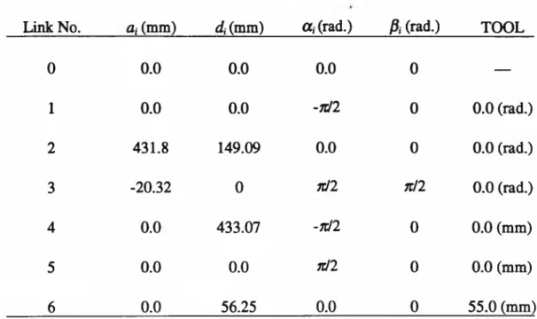
4.5 Kinematic Identification Results for a PUMA 560 Robot... 52

4.6 Chapter Summary... 64

CHAPTER 5. AUTONOMOUS CALIBRATION USING A TRIGGER PROBE...65

5.3 RNN-based Identification Algorithm...71

5.4 Data Collection...72

5.5 Results for a Puma 560 Robot...74

5.5.1 Simulation Results...75

5.5.2 Experimental Results... 81

5.5.3 Cross-Evaluation Using CMM...88

5.6 Chapter Summary & Discussions... 89

CHAPTER 6. GENERIC ACCURACY MODELLING USING FEEDFORWARD NEURAL NETWORKS...91

6.1 Introdction...91

6.2 A Generic Accuracy Function... ...93

6.3 Neural Network Architecture and Learning Algorithm...96

6.3.1 Neural Network Architecture...96

6.3.2 Network Learning Algorithm...99

6.4 Simulation Example for a One DoF Manipulator... 100

6.5 Network Training Using Experimental Data... 103

6.6 Chapter Summary... 110

CHAPTER 7. ROBOT ACCURACY COMPENSATION USING ARTIFICIAL NEURAL N ETW O R K S...

111

7.2 Non-parametric Accuracy Compensation... 113

7.2.1 Accuracy Compensation Using Polynomial Functions... 113

7.2.2 Accuracy Compensation Using Feedforward NN... 116

7.3 Model-based Accuracy Compensation... 124

7.3.1 Problem Formulation and Numerical Solutions... 124

7.3.2 RNN-based Algorithm for Accuracy Compensation... 127

7.3.3 Path Compensation... 130

7.3.4 Compensation Near Robot Singularity... 133

7.4 Chapter Summary... 140

CHAPTER 8. CONCLUSIONS AND FUTURE W ORK... 141

REFERENCES...146

APPENDIX... 158

Appendix 1 Forward Kinematic of Puma Robot & Orientation Represent... 158

Appendix 2 Closed-form Inverse Kinematic Solution of Pinna Robot... 159

Appendix 3 Ordinary Jacobian Matrix for Puma 560 Robot... 161

Appendix 4 Special Jacobian Matrix of Puma 560 Robot... 162

Appendix 5 Program for Data Collection Using a Trigger Probe... 164

Figure 1.1. Positioning Control of a Robot Manipulator...03

Figure 2.1. Biologically-inspired Neurocomputing Model...19

Figure 3.1. Denavit-Hartenburg Parameters for a Revolute Joint... 27

Figure 3.2. Relationship between Moving Frames and Base Frame... 31

Figure 3.3. Relationship between the Differential Changes of the End-effector Frame and the Differential Changes in the i-th Link Parameters... 32

Figure 4.1. Hopfield Neuron Circuit...41

Figure 4.2. Hopfield Analogue Neural Circuit Model...42

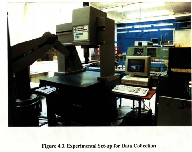
Figure 4.3. Experimental Set-up for Data Collection...47

Figure 4.4. Measurement Grid for Data Acquisition... 48

Figure 4.5. Schematic of Measurement Set-up... 49

Figure 4.6. The End-effector (Measuring Cube) Coordinate System... 50

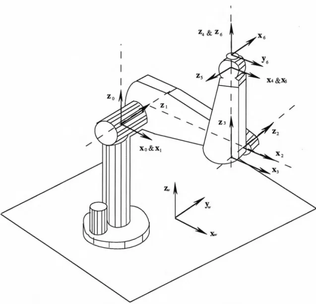
Figure 4.7. Puma Coordinate Frame Assignment...53

Table 4.1. Nominal Parameters of a Puma 560 Robot Using D-H Model... 55

Table 4.2. Identified Kinematic Parameter Errors of the Puma 560... 57

Table 4.3. Residual Error Comparisions Using the D-H Model... 57

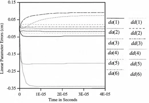
Figure 4.8. Time Evolution of Kinematic Error Identification... 58

Table 4.4. Nominal Parameters of a Puma Robot Using a Modified D-H Model ...61

Table 4.7. Residual Error Comparision Using the Modified D-H Model... 62

Figure 4.9. The Residual Position Errors Distribution for 100 Test Points... 63

Figure 4.10. The Relationship between the Observations and the Final RMS Errors...63

Figure 5.1. Constraint Conditions for Co-planar Points... 67

Figure 5.2. The Trigger Probe...73

Table 5.1. Nominal Parameters of a Puma 560 Robot... 75

Figure 5.3. Simulation Program Flowchart... 77

Table 5.2. Induced & Identified Kinematic Errors... 78

Table 5.3. Accuracy Comparisons for Calibration Points... 78

Table 5.4. Induced & Identified Kinematic Errors...80

Table 5.5. Accuracy Comparisons for Calibration Points... 80

Figure 5.4. Simulation Result with Induced Errors... 81

Figure 5.5. Experimental Set-up for Data Collection...83

Figure 5.6. Time Evolution of Kinematic Errors during Identification... 84

Table 5.6. Identified Errors of a Puma 560 Robot... 85

Table 5.7. Accuracy Comparisons Based on Test Points... ...85

Figure 5.7. Test Result with Experimental Data... 86

Figure 5.8. Z-axis Constraint Plane Perceived by the Robot Controller... 87

Figure 6.2. A Pi-sigma Network with One Output... 98

Figure 6.3. One Degree of Freedom Manipulator... 100

Figure 6.4. NN Representation of Generic Accuracy Model for a One DoF Robot... 101

Figure 6.5. Training and Implementation of NN Accuracy Model... 103

Figure 6.6. Neural Network Architecture for Accuracy Modelling... 104

Figure 6.7. Learning Curves for Positional Accuracy Modelling... 106

Figure 6.8. NN Generalisation Test for Position Compensation... 109

Table 6.1. Accuracy Evaluation for Pi-sigma Network based-on Test Points 109 Table 6.2. Accuracy Evaluation for Backprop. Net based-on Test Points... 110

Figure 7.1. Nonparametric Accuracy Compensation... 113

Figure 7.2. Training and Implementation of NN Accuracy Model...118

Figure 7.3. Neural Network Architecture for Accuracy Compensation...118

Figure 7.4. Learning Curves for Inverse Compensation... 120

Table 7.1. Inverse Accuracy Compensation Results of Puma Robot... 121

Table 7.2. Experimental Evaluation of Inverse Compensation Results... 121

Figure 7.5. Accuracy Improvement of Inverse Compensation... 123

Figure 7.6. Accuracy Compensation Along the Path... ...132

Figure 7.7. Robot End-effector and Wrist Singularity... 133

Figure 7.10. Joint Compensation Amount Near Singularity... 135

Table 7.3. Simulation Results for ¡j. = 101 in a Singular Configuration...137

Table 7.4. Simulation Results for // = 106 in a Singular Configuration...137

ANN (or ANNs, or NN) Artificial Neural Netwoks

BP Back-Propagation

CCD Charge-Coupled Device

CIM Computer-Integrated Manufacturing

CNC Computerized Numerical Control

CMAC Cerebellar Model Articulation Controller

CMM Coordinate Measuring Machine

CPC Complete and Parametrically Continuous

D-H Denavit-Hartenburg

DoF Degree of Freedom

FMS Flexible Manufacturing System

GA Genetic Algorithm

LMS Least Mean Square

LVDT Linear-Variable Differential Transformer

MLP Multi-Layered Perceptron

N-R Newton-Raphson

ODE Ordinary Differential Equations

PUMA Programmable Universal Machine for

Assembly

SVD Singular Value Decomposition

TCP Tool Centre Point

VLSI Very Large Scale Integrated-circuit

VSC Variable Structure Control

It was a meeting with a Napier delegation in Shenzhen (a booming city in the corridor between Hong Kong and Canton, Southern China), especially a conversation with Prof. James Murray, Vice-Principal of Napier University, that made me seriously consider the idea to pursue a PhD abroad. However, without the financial support from Napier University Scholarship, and CVCP (Committee of Vice-Chancellor and Principals of Universities of the United Kingdom) ORS (Overseas Research Student) award, the sparkled idea would have never come to fruition.

I would have not survived my first day in Edinburgh without help from Simon Liang, a PhD student from Taiwan, who was kind enough to drive to the airport to meet me in the early morning through the heaviest snow I had ever seen. Many thanks, Simon, for your friendliness and hospitality, as well as for many delightful discussions about Chinese culture and politics — the past and the future.

I am grateful to Dr John Hallam of Dept, of Artificial Intelligence, The University of Edinburgh for his instruction during the early stage of my research, which was invaluable in saving me from struggling in numerous murky ideas.

I would also like to acknowledge gratefully many other people for help and assistance during the course of my study. Among them are, Bill Campbell, for his assistance in robot programming; Heather Rea, for allowing me to use some of her data, and useful discussions; Ronnie Cohen, for his help with the use of Coordinate Measuring Machine; Dr Bob Stafford, for his tips on grammar and presentations; Bill Young, for being there when utilities were needed; and to all of my officemates, for tea-drinking time and entertainment.

I am indebted to my supervisors, Dr John Lewis, Dr Mike Mannion, Prof. Francis N-Nagy, Dr Barry Keepence, and Dr Duncan Marsh, for their inspiration, enlightenment and encouragement.

Last but not the least, I would like to thank my wife Du Ling, and my parents, for their love and consistent support.

Robot calibration is an integrated procedure of measurement and data processing to improve and maintain robot positioning accuracy. Existing robot calibration techniques require extensive human intervention and off-line processing, which preclude the techniques from being used to perform on-site calibration in an industrial environment at regular intervals. This thesis investigates and develops intelligent calibration processing algorithms and a novel measurement method toward rapid autonomous robot calibration in a shop-floor environment.

Artificial Neural Network (ANN) techniques have been vigorously investigated for calibration data processing (modelling, identification and compensation). A new identification algorithm has been developed for estimating robot kinematic parameter errors using Hopfield continuous-valued type Recurrent Neural Network (RNN). The RNN-based algorithm is computationally more efficient and robust compared with conventional optimisation approaches.

A generic accuracy model which accounts for various error sources was introduced. A higher-order neural network was used for implementation of the generic accuracy model. Due to the ANN learning capability, computational power and adaptability, the ANN-based accuracy representation offers an appealing solution to the complex modelling problem.

Efficient and robust accuracy compensation algorithms have been developed under the framework of artificial neural networks. The ANN-based algorithms provide constant-time inverse compensation therefore are suitable for on-line implementation. Both path compensation and compensation near robot singularity were tackled using the new algorithm.

A novel autonomous calibration tool was developed using a trigger probe and a constraint plane. The new method eliminates any use of external measuring devices to determine robot end-effector location measurements, enabling the robot to perform self-calibration on a production line. Robot accuracy was improved to the level of its repeatability within the local calibration volume using the new calibration scheme, which is consistent with the results from using a precision external measuring device, in this case a Coordinate Measuring Machine (CMM).

Ax = [dx, dy, dz, Sx, 5y, &]r P, = [Xi, yb z jr A, S T„ A, [n, s, o] [x„ yf, zü S — [flj, ûj ü„] d = [dl, d x ...,d„\

a = [al,

a„]

df_ df_ d(_ df_

dû' da

q = fà]

End-effector inaccuracy vector. The zth end-effector position vector. Position, and oriencation inaccuracy. End-effector homogenous transformation. The i-th link homogenous transformation. End-effector orientation vectors.

The j'-th coordinate system

Link offset vector,« is the number of DoF. Link length vector.

Link twist angle vector. Joint angle vector.

Kinematic (geometric) parameter vector. Kinematic error vector.

Special Jacobian matrix. Ordinary Jacobian matrix.

Position, and orientation error vector. Network energy function.

Network connection weight, and input, learning rate.

Scaling weight matrix. Residual error vector.

Regulation coefficient constant. Generalised joint variables. The z-th joint correction. Forward kinematic function.

The l-th weight, and bias correction. Network learning parameter.

Diagonal regulation weight matrix. Coefficient matrix of linear system. Aggregated inaccuracy vector. Side length of the measuring cube.

CHAPTER 1

1.1 Research Background and Motivation

The role played by industrial robots in modem factories is not as widespread as was predicted a decade ago. There are many reasons why robot systems have not met early expectations. One of the reasons is that most robot systems fail to deliver the promised flexible manufacturing environment. Industrial robots, as they currently exist, must be. taught even the most basic tasks required of them for operation in a complex and highly diverse human world. Programming or teaching a robot to perform a desired task is exceedingly labour intensive. Any minor change in the task or uncertainties which exist in the robot or the environmental set-up will invalidate, partially or completely, the developed programs. Off-line programming which supports the development of a robot program in a simulated environment has resulted from research seeking better robot programming methods. Robot positioning accuracy, however, is critical for off-line generated programs to be implemented successfully on a shop floor.

One major goal of robotics research is to instil some human-like intelligence in robots, enabling them to function autonomously in an unstructured environment. An intelligent robot must have the ability to adapt its behaviour quickly and effectively to unpredictable environmental changes without human intervention. To position its end- effector as precisely as desired in a changing environment is one of the fundamental capabilities for a robot to achieve high level intelligence or autonomy. To address robot motion control accuracy in particular and robot programming flexibility in general, a

great deal of research endeavour has been made in various areas ranging from automated task planning, fine-motion planning, error detection and recovery, to learning control and adaptive control, focusing on robot controller's performance enhancement. While many encouraging results in laboratory environments have been reported in these areas, it is generally believed that it will still be years before there is a major impact on the robot systems currently used in most manufacturing applications. Robot calibration is an approach that can improve robot positioning accuracy significantly without increasing the robot controller's complexity, and can be easily integrated with existing systems. As robot positioning accuracy is a highly complex problem dealing with various error sources which exist in changing environments, an intelligent calibration scheme is needed to make error sources robust with minimum human intervention.

An artificial neural network (ANN) is a new technique in the field of artificial intelligence which imitates the functional processes of the human brain. By taking advantage of the structure of the human brain, which features massive parallelism and high interconnectivity, it is hoped that extremely complex problems can be solved by neural networks. Due to their computational power, learning methodology, adaptability and fault tolerance, neural networks offer appealing solutions to intelligent robotic problems. In this thesis, artificial neural network techniques are applied to the robot calibration processes, aiming at autonomous robot calibration in a shop floor environment.

1.2 Robot Positioning and Calibration Problem

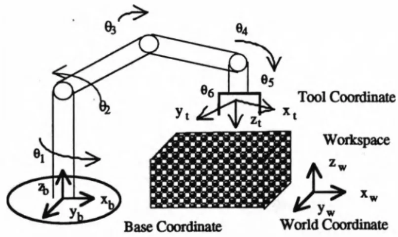
One of the basic capabilities of industrial robots is to position their end-effectors precisely so that they can perform manipulation tasks successfully. Precise positioning control is difficult for multi-joint articulated manipulators since they are open-chain mechanisms with coupling between motions of each individual link. The desired locations (or pose: position and orientation) of a robot end-effector are normally specified in Cartesian space (workspace), while these locations are achieved by controlling joint values (angles for revolute-joint robots) in robot joint space (Figure 1.1). The transformation from Cartesian space to joint space is called the inverse kinematics in robotics. The inverse kinematics problem is typically a computationally intensive procedure for general-form multi-link manipulators, the accurate solution of

which depends upon the algorithms used and upon precise knowledge of robot parameters.

In practice, most industrial robots are designed to have simple-form kinematics (Hayati and Roston, 1986) so that the inverse kinematics problems have analytic close- form solutions. For instance, the widely-used PUMA robot is designed so that the second and third joint axes are parallel and the last three joint axes intersected orthogonal in a point. The inverse kinematics of the PUMA robot is analytically solvable due to its special kinematic structure (Fu, Gonzalez and Lee, 1987; Craig, 1986); However, for a number of reasons (including manufacturing tolerance, repair and set-up errors, wear and tear, transmission errors, and compliance), the internal design model used in the robot controller will not accurately describe the actual relationship between robot workspace and joint space. Therefore, the actual locations achieved by controlling joint values, obtained from the controller's internal model, will deviate from the desired locations. Robot calibration is defined as a process of improving robot positioning accuracy through modifying robot control software without changing the robot's hardware configuration (Mooring, Roth and Driels, 1991). The modification of control software can be performed either in robot workspace (forward calibration), or in joint space by finding the corrected joint values to drive the robot so that the end-effector deviations can be minimised (inverse calibration) (Shamma and Whitney, 1987).

Several performance specifications are used to describe positioning characteristics of robot manipulators, which include accuracy, rep e a ta b ility, and resolution (Kozakiewicz, Ogiso and Miyake, 1990). The resolution is the smallest motion (linear and angular) the robot's end-effector can reliably execute. The repeatability is a measure of the robot's ability to return its end-effector to exactly the same point in workspace many times in succession. The (absolute) accuracy is a quantitative parameter describing the robot's ability to position its end-effector exactly in the World coordinate system. When a six degree of freedom (DoF) robot is issued a command to move its end-effector to a location P in workspace:

P[x, y, z, 6» By, 0J (1-1)

it will actually move to a location:

P '[x+dx, y+dy, z+dz, 9X+Sx, 6y+Sy, 6Z+Sz] (1.2)

By commanding the robot to move to the location P consecutively, each time the achieved location P ' will be slightly different from P due to the joint servo and actuator repeatability errors. The average values of the deviations [dx, dy, dz, Sx, 5y, &] from their mean are a measure of the robot's repeatability in a given direction in a given configuration.

If there were no other sources of errors in the robot except from the joint servo system, the average (mean) values of deviations [dx, dy, dz, Sx, dy, Sz\ would be zero. However, because of other error sources, such as geometric errors in the robot components, assembly errors, transmission errors, etc., the average positioning errors are always non-zero. Therefore, when a robot is sent to many different locations in its workspace, the variation in [dx, dy, dz, Sx, 5y, &] will be much larger than variations due to repeatability alone. The average values of the deviation in different configurations are a measure of the robot's accuracy in a given direction. For a six DoF robot, the position and orientation accuracy are defined as:

Aav = — t ^ d x f + d y f + dzf

nn

— l^ S x f + dy.+5z^

where dxb dyb dzb Sxh 5yb 5ztare linear and angular errors measured at randomly chosen locations (i = 1, 2 , m) in the specific region of the robot workspace. Root Mean Square Error (RMS) can also be used as another measure of accuracy. Robot position and orientation accuracy according to the RMS are defined as :

> a ii l — I ( d x . + d y - + d z - ) 1 m ¡=1 H j f— ¿ ( « x f + S yf + a z f) m /=i (1.5) (1.6)

Robot accuracy will always be positive according to the definitions above.

Another useful accuracy specification is standard deviation. Robot position and orientation standard deviations are specified as:

+ dyf+dz‘ - A J 1

With the definitions of average and standard deviation errors, there is 99.7% probability that the positioning error of the end-effector will be within the limits of the linear and angular error ranges as specified by Aa +3crA; and 8a+3 cr6 (Kozakiewicz, Ogiso and Miyake, 1990). The average and standard deviation errors as defined above, together with the absolute error measured by the maximum deviation, are used in this work to describe robot positioning (both linear and angular) accuracy.

Robot resolution and repeatability are determined by the joint servo and actuator system of the robot, therefore they can only be changed by modifying hardware design. Robot accuracy, however, is determined by the software of the robot (robot geometric model, forward and inverse kinematic control software), and can be improved by the robot calibration process. Robot repeatability is the limit of any robot calibration efforts. Hardware based robot teaching methods, such as manual teaching robot joints by using a teaching pendant, require only good repeatability so that the robot can return to the memorised location exactly time after time. Software based robot teaching (programming), such as off-line programs, require good absolute accuracy in addition to a good repeatability because the robot is controlled indirectly through a computer

model of the manipulator, so that an exact robot model is needed to ensure that the robot will move exactly where it is commanded. Most industrial robots have reasonably good repeatability but rather poor absolute accuracy. For example, the repeatability of the commonly used PUMA robot is 0.1-1 (mm), but its- accuracy is normally up to 10- 20 (mm). The aim of robot calibration is to improve robot position accuracy to the order of its repeatability.

1.3 Application of Robot Calibration

Robot calibration plays an increasingly important role in all areas of robot production, integration and operation within Flexible Manufacturing Systems (FMS). The utilities of robot calibration can be explained as follows (Bernhardt and Albright,

1993):

1) Implementing off-line planned and simulated robot tasks: Whilst off-line programming can reduce significantly robot programming time and avoid costly mistakes compared with on-line teaching methods, the discrepancies between the simulated environment and the actual physical workcell must be minimised through calibration before the off-line generated programs can be implemented on a shop floor.

2) Evaluating robot production: Robot accuracy can be achieved by manufacturing the robot closely to its design specifications at a minimum tolerance. However, high precision is a costly manufacturing demand. In addition, many specifications can not be explicitly evaluated after a robot is completely manufactured and assembled. Robot calibration, on the other hand, provides a practical and effective means of accuracy improvement by implicitly determining its physical parameters.

3) Improving control of robot motion: Robot control accuracy can be improved by incorporating the identified parameters into the robot controller. Advanced control strategies can also take advantage of the precise knowledge of model parameters for accurate motion control, e.g. in adaptive control, robot kinematic parameters are assumed to be known (Bennett, Geiger and Hollerbach, 1991). 4

4) Monitoring robot component wear: Once a robot is operating in a flexible manufacturing system, component wear-and-tear or repairs can detrimentally affect positioning accuracy. A periodic re-calibration can be performed to determine if repairs

are necessary and/or if programs need adjusting (re-programming). If a robot is replaced, robot re-calibration also enables replacement robots to share programs of the old robot with necessary adjustments.

A robot calibration system consists of two major subsystems: measurement and data processing. Requirements for the measurement and data-processing of calibration systems are different depending on the purpose of robot calibration and the circumstances under which it is performed. When a robot is to be calibrated on the shop floor, its environment can place severe limitations on measurement and identification capabilities. While an accurate and sophisticated global measurement device is desirable for accurate identification of all model parameters in a laboratory before robot installation, it may not be practical for robot re-calibration in a production line. There are a number of robot calibration systems commercially available which are mainly for robot calibration in a controlled laboratory environment (Silma Inc., 1992). A calibration system, which is suitable for rapid re-calibration at regular intervals over the lifetime of the robot in a shop floor environment, is still not available in practice. The aim of this research is to develop measurement and data processing techniques suitable for rapid and automatic calibration in the shop-floor environment at periodic time intervals.

1.4 Overview of Thesis

This thesis focuses on the application of artificial neural network (ANN) techniques in robot positioning accuracy modelling, identification and compensation processes. The aim of this research is to develop measurement and data processing techniques suitable for robot autonomous calibration in an industrial application environment. For the purpose of this thesis, autonomous calibration is defined as a fully automated process for the robot to improve its positioning accuracy using its internal sensor measurements on-site whenever and wherever necessary (after a certain period of robot operation and in the volume where high accuracy is required). The remainder of this thesis is organised as follows:

Chapter 2 reviews the previous work in the area of robot calibration and related techniques.

Chapter 3 introduces robot kinematics based on the Denavit-Hartenberg (D-H) parameter description. The linear error model and the special Jacobian matrix are derived using a geometric approach, which are the basis for kinematic identification. A modified D-H parameter notation using an extra rotation parameter for consecutive parallel joints is discussed.

Chapter 4 develops a new kinematic identification algorithm using Hopfield continuous-valued recurrent neural networks (RNN). The network energy function is constructed such that its minimum corresponds to the minimum least square error between the actual and desired end-effector locations. The network connection weights are determined directly from the nominal kinematcs and the network neuron states represent the kinematic parameter errors to be identified. A full-pose (position and orientation) measurement scheme using a coordinate measuring machine (CMM) is described. Kinematic identification results for a six DoF Puma 560 robot are obtained using the RNN-based algorithm and conventional optimisation approaches. The identification network finds optimal solutions within a few characteristic time constants of the neural circuit, even for the singular model and the measurements are constrained to a local volume. Issues about the optimal number of measurement points and the modelling of the robot base and tool are also discussed.

Chapter 5 presents a novel robot autonomous calibration method using a trigger probe. The new method eliminates the use of any other external measuring devices to determine the robot end-effector location measurements, thus it is suitable for a periodic robot re-calibration on a production line. The kinematic constraint conditions are obtained from the known shape of the constraint surfaces, rather than from known reference locations as used by other researchers. The fully automated data collection scheme is described in detail. Kinematic identification is performed using the developed RNN-based algorithm. Both simulation and experimental results for a PUMA robot are presented, which show that robot positioning accuracy can be improved to the level of repeatability using the proposed method.

Chapter 6 discusses the development of a robot generic accuracy model which accounts for various error sources using feedforward neural networks. The generic accuracy function is introduced based on an expansion of the Fourier series, which serves as the basis for the design of a neural network architecture. The Pi-sigma network architecture is used as a generic model for robot accuracy problem because of its capability to generate higher-order trigonometric polynomial approximations

efficiently and dynamically, which is suited to the structure and the order of the generic accuracy function. Results for a six DoF Puma robot within a local volume of workspace are presented, and compared with the results of accuracy modelling using a Back-propagation network.

Chapter 7 focuses on robot accuracy compensation using ANNs, this being a subset of the inverse kinematics problem of the calibrated robot. A Pi-sigma feedforward network is used to approximate the relationship between robot nominal joint configurations and joint compensation. The trained network is used to perform a constant-time inverse compensation. While the feedforward network is effective for robot inverse compensation in a small portion of robot workspace, its training efficiency and accuracy is compromised if a large calibration volume is considered. For robot accuracy compensation which involves a large number of work points, the inverse compensation problem is reformulated and the Hopfield type recurrent neural network (RNN) is applied to the design of a robust and efficient accuracy compensator. The derivation of the RNN-based compensation algorithm is similar to that of kinematic identification, with the difference being the structure of the Jacobian matrix and the interpretation of neuron states. The RNN-based inverse compensation algorithm takes advantage of the a priori knowledge of kinematic structure therefore requires no training, and finds an accurate solution efficiently. Both path compensation and compensation near robot singular configurations are solved successfully using the RNN-based algorithm, and are compared with the widely-used Newton-Raphson approach.

CHAPTER 2

REVIEW OF PREVIOUS WORK

2.1 Methods of Robot Calibration

There has been extensive robot calibration research over the past decades and good reviews of the subject can be found in (Roth, Mooring and Ravani 1987), (Hollerbach 1989) and (Mooring, Roth and Driels 1991). Calibration methods can be classified as model-based parametric calibration and model-free non-parametric calibration. Most work on model-based parametric calibration has concentrated on kinematic model- based calibration or simply kinematic calibration (Hayati 1983; Wu 1983 1984; Stone 1986; Hollerbach 1989; Zhuang 1989; Mooring, Roth and Driels 1991), while a few papers have also taken non-geometric factors such as backlash, gear eccentricity, and joint compliance into account (Whitney, Lozinski and Rourke 1986; Judd and Knasinski 1991). In the category of model-based calibration methods, geometric and/or non-geometric factors are modelled and identification techniques are applied to identify the model parameters. The identified parameters are then used in algorithms for on-line compensation. In the category of non-parametric calibration, instead of modelling and identifying specific error sources, numerical fitting methods are adopted to approximate robot inaccuracy data which has been collected from local workspace (Shamma and Whitney 1987; Kozakiewicz, Ogiso and Miyake, 1990; Rea 1992). It is difficult to judge which method is better since the relative contributions of geometric and non- geometric errors to robot inaccuracy vary from one particular robot to another. While Whitney et al (1986) reported that non-geometric errors are as significant as geometric errors in affecting robot accuracy for a geared robot (PUMA 560), Judd and Knasinski

(1991) showed that as much as 95% of robot inaccuracy arises from geometric errors. Veitschegger and Wu (1987,1988) found that non-geometric errors only accounted for less than 0.3 (mm) of PUMA robot inaccuracy, which is in agreement with the result by Stone, Sanderson and Neuman (1986).

Generally kinematic model-based calibration is considered as a global calibration method which improves robot accuracy across the whole volume of robot space, while non-parametric calibration is a local calibration method which only works within a portion of the robot workspace. However, no clear boundary line can be drawn between these two categories of calibration. Kinematic calibration can be regarded as non-linear regression which uses kinematic functions as its basis functions. Kinematic parameters identified with data collected from the local workspace may perform better in the specific workspace than in the total work volume. This implies that these parameters do not necessarily represent the real parameters of the robot over the entire workspace but are the best fitting for the collected data in a least square sense. Therefore, some non- geometric factors can also be compensated in kinematic calibration by collecting enough data and choosing an adequate model. For most robot tasks, only accuracy over a subset of robot workspace is critical, in which most fine motions such as assembly operations are executed. As we concentrate on robot on-site calibration over a local area of robot workspace, both kinematic model-based calibration and non-parametric calibration are studied and evaluated in this work.

2.2 Kinematic Model-based Calibration Methods

Generally kinematic calibration consists of four sequential procedures: 1) modelling, 2) measurement, 3) identification, and 4) compensation, enabling precise kinematic parameters to be identified thus leading to improved accuracy. These procedures are described below. Related work has been reviewed and categorised on the basis of their primary emphasis.

1) Modelling:

A kinematic model is a mathematical description of the geometry and motion of a robot. Choosing a kinematic model to describe the relationship between robot joint space and its workspace co-ordinates is the basis for the kinematic model-based robot

calibration. Denavit-Hartenburg (D-H) homogenous transformation is a mathematical tool adopting four parameter pairs to describe the spatial relationship between manipulator workspace and joint space co-ordinates (Denavit and Hartenberg, 1955). Early work on robot calibration concentrated on robot accuracy model development based on D-H representation (Wu, 1983, 1984; Ibarra and Perrier, 1986; Zhen, 1985). Mooring (1983) and Hayati (1983) pointed out the model singularity problem inherent in the D-H formalism. Parameter jumps occur in the identification process when the D- H modelling convention is used to describe two consecutive nominally parallel axes. A modification to D-H modelling was proposed by Hayati (1983) by incorporating an extra rotation parameter for parallel revolute axes. Similar modifications were reported subsequently by Veitschegger and Wu (1986), and Judd and Knasinski (1987).

Many other alternative kinematic models have also been proposed for robot calibration. Examples of these include: the 'zero-reference model' by Mooring and Tang (1984) which avoids model singularity by not using a common normal as a link parameter; the S-model by Stone, Sanderson and Neumann (1986) which uses six parameters for each link to allow an arbitrary placement of link coordinate frames; the shape matrix model by Broderic and Cipra (1988) and Ziegert and Datseris (1990) which separates the joint variables from other link parameters based on screw theory as described by Suh and Radcliffe (1978); the CPC model by Zhuang (1989) and Zhuang, Wang and Roth (1993a,b) which is complete and parametrically continuous as it is defined for manipulator calibration. However, the kinematic models used in most existing robot controllers are still based on D-H notations. The alternative models designed for calibration need to be converted back to D-H equivalent parameters after calibration for model consistency consideration.

2) Measurement

Experimental measurements of robot end-effector locations are collected using external co-ordinate measuring devices in this phase. The actual measured locations of the robot end-effector are then compared with the locations predicted by the theoretic model to obtain the workspace inaccuracy data.

Measurement is the most difficult and time-consuming phase of robot calibration. A variety of measurement methods have been used and a survey of major techniques

designed for robot test and calibration can be found in (Lau, Dagalakis and Myers, 1988). Such techniques include the use of co-ordinate measuring machines (Driels, Swayze and Potter, 1993; Zhuang, Wang and Roth, 1993b), visual and automatic theodolites (Chen and Chao, 1986; Whitney, Lozinski and Rourke 1986; Judd and Knasinski, 1991), servo-controlled laser interferometers (Lau, Hocken and Haynes, 1985; Prenninger, Vincze and Gander, 1993; Mayer and Parker, 1994), acoustic sensors (Stone, Sanderson and Neuman 1986, and Stone 1992) and visual sensors (Tsai and Lenz, 1989; Zhuang, Wang and Roth, 1993a). The measurement devices vary considerably in their cost, ease of use and accuracy, but they all have certain drawbacks which include:

• The measuring techniques are mainly designed for robot calibration in a well- controlled laboratory environment. The robot has to be removed from its normal operating environment in order to perform the calibration.

• Trained personnel are required to operate the measuring devices properly. • Data collection is time-consuming and difficult to automate.

• Set-up and measurement processes require a lot of human intervention. Therefore,, these techniques are not suitable for robot on-site calibration in an industrial application environment.

It is known that partial pose information of robot end-effector is sufficient for complete kinematic parameter identification. Tang and Mooring (1992) utilised a mechanical fixture to obtain partial information of a robot end-effector location. The fixture consists of a flat plate with some accurately located points on it. An end-effector is designed with a flat surface at a known angle to the last axis of the robot. In the 'free' mode of the robot, the robot end-effector was manually moved to the known points of the plate and against the flat plate such that components of the end-effector position and orientation were 'measured'. Veitschegger and Wu (1988) calibrated a PUMA robot based on the use of the similar plate fixture with a set of precisely positioned holes. The end-effector with a pointing device was moved passively to the holes to make point measurements. The partial pose measurement scheme eases the requirements for measuring devices. The low cost and elimination of large-sized external measuring device make it appealing for on-site applications. However, the measuring process is not automatic and requires intensive human intervention. The success of such a scheme

also relies on the predetermined locations of reference points on the fixture. In addition, as pointed out by Driels and Swayze (1994), not every robot provides a 'free* mode in which the manipulator can be moved manually while the joint encoders are powered up and the joint servos are disabled.

The approach to use physical constraints in the workspace was further developed by Bennett and Hollerbach (1990, 1991), who proposed that a passive mechanism be used to transform the open-loop manipulator into a closed kinematic chain. The concept of autonomous robot calibration was introduced which was defined as the automated process of determining a robot's model by using only its internal sensors (Bennett, Geiger and Hollerbach, 1991). It has been observed that autonomous calibrations are possible for robot manipulators with either some a priori knowledge of the task constraint or redundancy of the sensing systems (e.g., adding additional links or joints to connect robot end-effector and ground, or two robots gripping together to form kinematic chain closure). Based-on these observations, the automated data collection schemes were proposed for robot calibration using LVDT (linear-variable differential transformer) ball bar system (Goswami, Quaid and Peshkin, 1993) or wired potentiometer (which can be considered as a flexible ball bar system) (Driels and Swayze, 1994) connecting the robot end-effector to the known reference point in the ground. Closed-loop constraints were formed for kinematic identification by obtaining accurate radial measurements of the ball bar or the wired potentiometer. But special fixtures are needed for such a system, which may require painstaking efforts to set up; and the added fixtures are rather difficult to model.

Autonomous calibration of hand-eye systems has also been performed by using robot joint readings and camera co-ordinate measurements to form the closed-loop constraints (Tsai and Lenz, 1989; Bennett, Geiger and Hollerbach, 1991; Zhuang, Wang and Roth, 1993a). The drawbacks for autonomous calibration of hand-eye systems are that not all robotic applications incorporate a visual camera as part of the system; and the camera measurements are known to be insufficiently accurate for manipulator calibration covering a large workspace volume. Another kind of task constraint has been proposed for robot kinematic parameter identification which utilised laser line tracking in the robot workspace (Newman and Osborn, 1993). While the motion of the robot tip-point was constrained to a line motion in the workspace, the robot joint values were recorded for kinematic identification. But only simulation results for a planar two-link manipulator were presented. An active and fully

autonomous calibration scheme was proposed by Zhong and Lewis (1995) which uses a trigger probe to touch a constraint surface in a workspace. The constraint conditions are obtained from the known shape of the constraint surface rather than the known locations of reference points. This autonomous calibration scheme will be discussed in depth in Chapter 5.

3) Identification

Kinematic parameter errors are identified in this phase by minimising the collected workspace inaccuracy in the least mean square sense. Kinematic identification is basically a standard non-linear or linear least square optimisation procedure. Non-linear algorithms do not require the identification Jacobian and are computationally more robust but more computation time is required for convergence. Linear least square algorithms require less computation time to converge but suffer from numerical problems of ill-conditioning of the identification Jacobian. Robust minimisation techniques such as the Levenberg-Marquardt algorithm have been applied to cope with the problem at the expense of computation time (Bennett and Hollerbach, 1991; Mooring and Padavala, 1989). More advanced parameter estimation techniques are also applied in kinematic identification. A maximum likelihood estimator was used by Renders et al (1991). Mooring, Roth and Driels (1991) applied Kalman Filtering techniques to investigate the relationship between calibration accuracy and measurement noise.

To improve kinematic identification robustness and efficiency, some theoretic issues have been addressed by a number of researchers. Kinematic identifiability was defined by Bennett and Hollerbach (1991). Meng and Borm (1988) introduced an observability index to find the optimal measurement configurations for robot calibration, while Khalil, Gautier and Enguehard (1991) used the condition number of the identification Jacobian to determine optimum calibration configurations. Experimental and simulation studies were performed by Borm and Menq (1989, 1991) and Pathre and Driels (1990) to demonstrate the importance of observability to kinematic identification. Determining the optimal configurations for robot calibration according to the observability criteria is a high dimensional non-linear optimisation problem. An advanced optimisation technique, simulated annealing, was used by Zhuang, Wang and Roth (1994) for off­ line selection of measurement configurations. Generally the optimal measurement

configurations determined by using the observability index are that the measurement points should spread across the whole workspace as widely as possible. This observation is useful for robot calibration performed in the laboratory environment where the robot can be controlled to move to arbitrary configurations. For robot on-site calibration in a crowded industrial environment, the calibration movement of robots is normally constrained. Given the limitation of constrained movement for data collection, numerically more robust and efficient algorithms are needed for robot on-site calibration processing. A Hopfield-type recurrent neural network(RNN)-based algorithm was proposed by Zhong and Lewis (1994) for efficient and robust kinematic identification, which is the focus of Chapter 4.

4) Compensation

Implementation of the identified kinematic model is the final and crucial stage of kinematic calibration. Due to the difficulty in modifying kinematic parameters in the robot controller directly, joint compensations are made to the encoder readings of the robot obtained by solving the inverse kinematics of the calibrated robot. The assumption of simplified kinematic structure which applies to the nominal robot is no longer valid for the calibrated robot due to kinematic parameter changes. Therefore the inverse kinematics of the calibrated robot is generally not analytically solvable. Numerical algorithms such as the Newton-Raphson approach are normally adopted to find the joint corrections needed to compensate for Cartesian errors (Kirchner, Gurumoorthy and Printz, 1987; Mirman and Gupta, 1992). However, the Newton- Raphson method is based on iterative inversion of the compensation Jacobian, therefore on-line compensation is problematic due to the computation expense, and the algorithm breaks down in the vicinity of robot singular configurations. The differential transformation compensation algorithm was presented by Veitschegger and Wu (1988), in which two nominal inverse problems are solved for one task point compensation. A comparison of various compensation algorithms was made by Vuscovic (1989). Zhuang, Hamano and Roth (1989) who formulated the accuracy compensation as a linear optimal control problem such that the linear quadratic regular method was applied to the design of a robust accuracy compensator. Existence and uniqueness are ensured in robot configurations near singularities by adding a regulation term to the performance index. The computation of the linear quadratic regulator algorithm is rather expensive, though simplification can be made in special cases. Zhong and Lewis

(1994), and Zhong, Lewis and N-Nagy (1995) presented neural network-based algorithms for inverse compensation. The neural network-based inverse compensation algorithms will be discussed in detail in Chapter 7.

2.3 Non-parametric Calibration Methods

Model-based parametric calibration is limited by the inability to model and identify all error sources which contribute to robot inaccuracy. Non-parametric calibration, on the other hand, employs non-parametric methods to establish an approximation function based on a sufficient number of measurement data collected from the local volume. Shamma and Whitney (1987) distinguished between forward calibration, which determines the end-effector location from joint angles, and inverse calibration, which determines the joint angles from the end-effector location. The inverse calibration was considered by Shamma and Whitney, in which the third-order trivariate polynomials were applied as approximation functions to relate the end-effector location to joint angles. The single calibration of a six DoF PUMA robot was separated into two calibrations, which comprised the first three major DoF calibration and then the remaining three minor DoF calibration. The training data points were generated by Tchebychev spacing in one quadrant of the robot workspace. Simulation showed that accuracy was reduced to below 0.3 (mm). Direct extension of the three DoF robot to a general robot would be difficult due to the limitation of polynomial approximations. In the case that a higher DoF are considered, the polynomial functions required will be too complex to be determined by the least square solutions, and would require a large number of data points which are practically difficult to obtain.

Mooring , Roth and Driels (1991) discussed a table lookup scheme for a simple two- link planar robot based on CMAC (Cerebellar Model Articulation Controller), which was originally developed by Albus (1975a,b) to model the function of the cerebellar cortex of the brain, but it can also be used as a general purpose function approximator. Even for a simple two-link planar robot, CMAC implementation of inverse kinematics exhibited unacceptable low accuracy and poor interpolation ability, and required a large number of training points. It concluded that CMAC scheme is still not ready to use for multiple joint robots. Another table lookup scheme was proposed by Everestt and McCarroll (1986) which was based on a finite element method.

Kozakiewicz, Ogiso and Miyake (1990) applied a multi-layered neural network approximation of the joint corrections for a four DoF Scara robot. Simulations were performed which included non-geometric model such as joint compliance. Comparisons with the polynomial approximations showed that the neural network gave poor accuracy. More recently, Miyazaki, Maekawa and Bamba (1992) proposed a hybrid compensation method to improve positioning accuracy of industrial robots by introducing a feedforward layered neural network in addition to the conventional kinematic model. The maximum position error for test points was improved from 17.67 (mm) before compensation to 1.73 (mm) after kinematic calibration, to 4.30 (mm) after neural network compensation, and to 1.01 (mm) after both kinematic calibration and neural network compensation were used. Only forward calibration was discussed and inverse compensation was not addressed. Zhong, Lewis and Rea (1994) proposed a generic accuracy compensator for industrial robots based on the Pi-sigma neural network. The ANN-based accuracy compensation eliminates the need for model-based calibration, with the various error sources being represented in the distributed network weight connections. The ANN-based forward compensation will be discussed in Chapter 6 and the inverse compensation discussed in detail in Chapter 7.

2.4 Artificial Neural Network Techniques

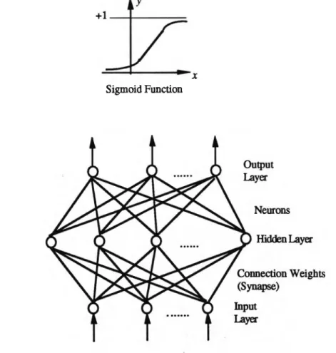
Artificial Neural Networks (ANNs) have emerged from studies of how human and animal brains perform operations. The human brain is made up of many millions of individual processing elements, called neurons, that are highly interconnected. Artificial neural networks are made up of individual models of the biological neuron (artificial neurons or nodes) that are connected together to form a network. The neuron models that are used are typically much simplified versions of the actions of a real neuron. Information is stored in the network often in the form of different connection strengths, or weights, associated with the synapses in the artificial neuron models. A neuron model processes information by summing the weighted inputs to the neuron and passing the result through some non-linear activation functions such as a sigmoid function to an output.

There are many types of neural network available, depending on the specific arrangements of artificial neurons and their interconnections. The most widely used neural network architecture is the Multi-Layered Perceptron (MLP) because of its

simplicity. The network consists of an input layer, a number of hidden layers (typically only one or two hidden layers are used) and an output layer as shown in Figure 2.1. Data flows through the network in one direction only, from input to output; hence, this type of network is called a feedforward network. The most common training algorithm for the network is back-propagation algorithm originally proposed by Werbos (1974) and Rumelhart, Hinton and Williams (1986). An important feature of the MLP is that this network can accurately represent any continuous non-linear function relating inputs and outputs (Homik, 1991; Homik, Stinchcombe and White, 1990). Hence, the MLP network exhibits potential for many applications which can be formulated as a non­ linear mapping problem. Other famous neural network architecture include Hopfield networks (Hopfield and Tank, 1986); Counter-Propagation networks (Hecht-Nielsen,

1990); and self-organising Kohonen networks (Kohonen, 1984), etc.

Sigm oid Function

Figure 2.1 Biologically-Inspired Neurocomputing Model — Multiple-Layered Perceptron with One Hidden Layer

2.5 Artificial Neural Network Applications in Robotics

A variety of uses for ANNs related to robotics and control have recently been reported. The use of ANN control is particularly suited to problems related to the control capabilities of animal nervous systems, and robot inverse kinematics transformation application naturally fall into this domain of applications. One of the earliest ANN approaches to robot control is due to Albus (1975b). The basic idea of his CM AC scheme for robot control is to compute control commands by look-up tables rather than by solving control equations analytically. While the CMAC has a computational advantage over conventional approaches due to its distributed fashion, it requires a large size of computer memories for multiple DoF robot, and is not able to perform interpolations. Kuperstein (1988) concerned himself with models of visual motor coordination in robots. While he did not explicitly address the inverse kinematics problem, his work did in fact use neural networks to obtain the transformation needed to convert desired hand coordinates in Cartesian space into appropriate joint coordinates. A neural controller called INFANT, which learns sensory-motor coordination from its own experience, has been reported which achieved an average positioning accuracy of 3% of the arm's length in position and 6 degrees in orientation (Kuperstin and Rubinstein, 1989). Other attractive features of the INFANT include real­ time operation, learning and maintaining its own calibration, and fault tolerance.

Inverse kinematic control has also been studied by a number of researchers, e.g., Guez and Ahmad (1988), Josin (1988) and Josin, Chamey and White (1988), using back-propagation learning algorithms for feedforward networks. However, the back- propagation network-based inverse kinematics solutions are typically not accurate enough for practical applications even for 2 or 3 DoF robots. Attempts to apply back- propagation directly to systems with more DoF have not been very successful (Kozakiewicz, Ogiso and Miyake, 1991; Daunicht, 1991), since these systems typically exhibit high-order nonlinearities and hence very slow learning rate and unacceptable learning accuracy. To exploit both ANN efficiency and numerical accuracy, Ahamad and Guez (1990) proposed a hybrid approach that used the ANN outputs as a initial solution for iterative numerical Newton-Raphson method, which resulted in a reduced number of iterations of the numerical method.

All the papers cited above concentrate on position-based inverse kinematic control where only position (location) information needs to be converted. In velocity-based inverse kinematic control or Jacobian control (Fu, Gonzalez and Lee, 1987), both position and velocity information needs to be transformed from Cartesian space to joint space. Velocity-based inverse kinematics is much more complex than position-based inverse kinematics since the number of input variables is doubled. The network training problem may become intractable with the increase in the dimensionality of the input space since the input space will experience an exponential growth in size (Yeung, 1989). Following the divide-and-conquer principal, Yeung (1989), and Yeung and Bekey (1989) proposed context-sensitive networks which partitioned the set of input variables into two groups. One set is used as the input to the network which approximates the basic mathematic operations being represented (the function network), while the second set determines the setting or context within which the function is determined (context network). They have shown that context-sensitive networks improved learning accuracy and reduced convergence time drastically compared with the standard back-propagation networks. Similar network architecture has been used by Bassi and Bekey (1989) to extend the work to inverse dynamics learning. A complete solution to the inverse dynamics problem has been presented by Miyamoto, Kawato, et al (1988). With a priori detailed knowledge of the dynamics equation for a three DoF robot, they decomposed the network into 26 sub-networks according to the primitive non-linear function terms in the analytic dynamic equations. The performance of the system is excellent due to the simplification of the learning task for sub-networks, which is equivalent to the determination of the coefficients in the dynamics equations.

The Hopfield type recurrent neural network (RNN) architecture (Hopfield and Tank, 1986) has been applied to the velocity-based inverse kinematics problems for robots with redundant DoF. Guo and Cherkassky (1989) implemented the Jacobian control scheme using the Hopfield analogue (continuous-valued) computation model. The states of neurons represent joint velocities of a manipulator, and the connection weights are determined from the current value of the Jacobian matrix. The network energy function is constructed so that its minimum corresponds to the minimum least square error between the actual and desired joint velocities. Simulation shows that the method is capable of solving the inverse kinematics problem for a planar redundant manipulator in real time. In contrast to the feedforward neural network-based inverse kinematics solutions, the RNN-based algorithm, by taking advantage of the kinematic structure of

the specific robot, requires no training and can find quality solutions within a few characteristic time constants of neural circuits. Li and Jiang ( 1993) extended Guo and Cherkassky's work by integrating the optimising properties of the RNN-based inverse kinematic control and the technique of the Variable Structure Control (VSC). The pseudoinverse Jacobian control scheme was implemented using an RNN algorithm for a planar redundant robot (Wu and Wang, 1994).

Other neural network architecture have also been vigorously investigated for robotic applications. Martinez, et al (1990) have shown that an extension of Kohonen's algorithm (Kohonen, 1984) for the formation of topological correct feature maps, together with an error-correction rule of the Widrow-Hoff type, can learn to control the robot arm and gripper movement by using only the input signals of two cameras. Wu, Jiang and Shiau (1993) used the modified two-layered counter-propagation network (Hecht-Nielsen, 1990) to control a robot's gross motion (first layer) and fine motion (second layer). The counter-propagation network, which combines the Kohonen self- organising feature map with the Grossberg outstar map (Grossberg, 1982), can be a statistically optimal self-programming lookup table for the adaptive control of robots. However, these neural network learning algorithms belong to unsupervised learning therefore they are not associative (Yeung, 1989). This implies that the training of such networks normally requires a large number of training data and the interpolation ability of the trained networks are typically poor. A more comprehensive review on the various ANN architecture and their applications in robot task planning, path planning, and sensor/motor control can be found in Kung and Hwang (1989).

2.6 Conclusions

Previous work on robot calibration and related techniques have been reviewed in this chapter. Although a great deal of research has been done on robot calibration over the past decade, most of the calibration techniques developed are only suitable for robot calibration within well-controlled laboratory environments. Rapid autonomous robot calibrations within a shop floor environment, although highly desirable, are still not available in practice. Efficient and robust data processing techniques and fully automated data collection methods are required to perform on-site calibration on a regular basis and within local workspace. Artificial neural networks are appealing for robot calibration processing including modelling, identification and compensation, due to their computational power, learning abilities, and fault tolerance. Selection of neural

network architecture are critical for their successful applications in robotics and a priori model knowledge are useful for designing NN architecture. A measurement method capable of collecting data from a local workspace automatically using portable physical constraints needs to be developed for on-site calibration,

CHAPTER 3

ROBOT KINEMATICS AND KINEMATIC ERROR MODELLING

3.1 Introduction

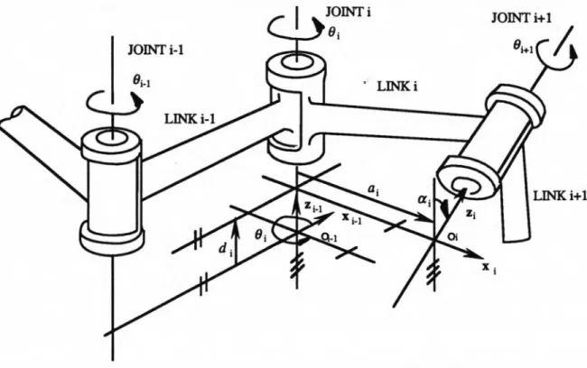
Robot tasks are normally described in terms of the relative locations (positions and orientations) of the workpieces and equipment which exist in the working environment. The study of kinematics reveals that the relative locations of objects can be defined clearly by attaching co-ordinate frames to each object so that when the object moves, so does the frame. The spatial transformation between robot end-effector location and its individual link geometry and joint movement is established in terms of the assigned Cartesian co-ordinate frames fixed relative to each of the links. The (4 x 4) Homogenous transformation matrix introduced by Denavit and Hartenberg (1955) and later adopted by Paul (1982) has become the most common approach to describing spatial transformations in robotics. In this chapter, we will review the Denavit- Hartenberg (D-H) method for robot kinematic modelling, and later develop a kinematic error model which describes the relationship between robot kinematic parameter variations and the predicted end-effector location error, which is the basis for kinematic calibration.

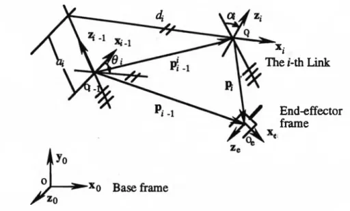
The kinematic error model for a single link is normally derived using the analysis approach of the homogenous transformation matrix and then applying it to the entire robot. The analytic expression of the coefficient matrix which gives a linear relationship between the kinematic parameter errors and the end-effector error was derived by Wu (1984) and Veitschegger and Wu (1986). The coefficient matrix has

been termed by Mirman and Gupta (1992) as a special Jacobian matrix which has been derived using a similar approach. A disadvantage of using the analysis approach is that the derivation requires a lot of mathematical operations and geometric interpretation is not obvious. Vuscovic (1989) presented a geometric expression for the special Jacobian matrix and termed it differently as kinematic sensitivities, but no derivation process was given. In section 3.3, a geometric approach to deriving the kinematic model is developed based on the theory of rigid body kinematics with moving (translating and rotating) co-ordinate frames. The geometric approach to formulating the special Jacobian matrix is straightforward and the geometric interpretation of the Special Jacobian is useful for identifying model singularities. The D-H model singularity for consecutive parallel revolute joints is then discussed. Finally, a modified D-H notation which overcomes the model singularity is introduced for use in following chapters.

3.2 Kinematic Modelling Using Denavit-Hartenberg Model

For robot manipulators with general kinematic structure of linkages, their complex spatial orientation and position can be specified by allocating kinematic frames to each of the robot links and then specifying transformation from one link to another. Denavit' and Hartenberg (1955) interpret the sequential transformation from one link to another as a multiplicative operation of (4 x 4) matrix:

T„ = A1*A2*...*Ai*...*A„ (3.1)

where T„ is a (4 x 4) homogenous transformation matrix which has the form:

" x * x Ox P x

n >

S7

0 0 0 1

(3.2)

and in terms of its vector components, n = [nx n, n j r, s = [j xsyjJ 7, o =[ox oy o J rare three unit vectors specifying the orientation of the x, y and z axis of the co-ordinate frame associated with T„ with respect to a reference frame, while p = [px py p j r specifies the position of the origin of that frame in a reference frame. For robot manipulators with n-links, the co-ordinate frame associated with T„ is normally attached to the robot end-effector frame while the reference frame is the robot base