Deep Generative Models for Semi-Supervised Machine Learning

General rights

Copyright and moral rights for the publications made accessible in the public portal are retained by the authors and/or other copyright owners and it is a condition of accessing publications that users recognise and abide by the legal requirements associated with these rights.

 Users may download and print one copy of any publication from the public portal for the purpose of private study or research.  You may not further distribute the material or use it for any profit-making activity or commercial gain

 You may freely distribute the URL identifying the publication in the public portal

If you believe that this document breaches copyright please contact us providing details, and we will remove access to the work immediately and investigate your claim.

Deep Generative Models for Semi-Supervised Machine Learning

Maaløe, Lars

Publication date: 2018

Document Version

Publisher's PDF, also known as Version of record

Link back to DTU Orbit

Citation (APA):

Maaløe, L. (2018). Deep Generative Models for Semi-Supervised Machine Learning. Kgs. Lyngby, Denmark: DTU Compute. DTU Compute PHD-2018, Vol.. 472

Semi-Supervised Machine Learning

Lars Maaløe

Kongens Lyngby 2018 PhD-2018-472

Richard Petersens Plads, building 324, 2800 Kongens Lyngby, Denmark Phone +45 4525 3031

[email protected] www.compute.dtu.dk

The reintroduction of deep neural networks has a large impact on the modeling capabilities of modern machine learning. This reignites the general public’s dream of achieving artificial intelligence, and spawns rapid progress in large-scale industrial machine learning development, such as autonomous driving. However, the leaps in development are still confined to a rather limited learning domain, in which labeled data is required. Labeled data is hard and costly to acquire, due to the amount needed to efficiently learn a modern machine learning model, and that many data sources are not directly interpretable. Consequently, research in different learning paradigms that utilize vast amounts of unlabeled data is getting more and more attention. Albeit possessing intriguing theoretical properties, machine learning models that learn from unlabeled data are still an unsolved research topic.

The thesis comprises methods that utilize the power of deep neural networks to learn from both labeled and unlabeled data. A background for the theoretical foundation of the proposed methods are described and empirical results showing their capabilities within generation and classification tasks are presented. Fi-nally, a real-life application within condition monitoring for sustainable energy is demonstrated, proving that the proposed methods have the expected impact and are applicable.

Re-introduktionen af dybe neurale netværk har haft stor indflydelse på mo-delleringskapaciteten i den moderne maskinlæring. Det har aktualiseret offent-lighedens efterspørgsel af kunstig intelligens, hvilket har medført signifikante fremskridt i den industrielle udvikling af maskinlæring, for eksempel inden for selvkørende biler. Udviklingen har dog været begrænset til et indskrænket læ-ringsdomæne, hvori der kræves annoteret data. Store mængder af annoteret data er vanskelige og dyre at erhverve, og det er ikke muligt at fortolke mange datakil-der for at skabe en modatakil-derne maskinlæringsmodel. Det resulterer i, at forskning inden for andre læringsparadigmer, der udnytter store mængder ikke-annoteret data, får stadig større opmærksomhed. På trods af at maskinlæringsmodeller der lærer fra ikke-annoteret data, har spændende teoretiske egenskaber, er det dog stadig et åbent forskningsfelt.

I denne afhandling præsenterer vi metoder, der udnytter mulighederne i neu-rale netværk til at lære fra både annoteret og ikke-annoteret data. Vi giver en baggrund for det teoretiske grundlag for de foreslåede metoder og præsenterer empiriske resultater, der viser metodernes evne inden for genererings- og klas-sifikationsopgaver. Endelig præsenterer vi en applikation inden for bæredygtig energiovervågning, hvori vi viser, at de foreslåede metoder virker.

This thesis was prepared at the Department of Applied Mathematics and Com-puter Science, Technical University of Denmark, in fulfilment of the require-ments for acquiring a PhD in Engineering.

During the PhD, a research stay was conducted at Apple Inc., Cupertino, Cali-fornia, USA. The research considered machine learning in autonomous systems, from which the findings are not disclosed in this thesis.

The thesis was funded by the Technical University of Denmark and Innovation Fund Denmark with guidance under Professor Ole Winther. The work was carried out between December 15, 2014 and March 17, 2018.

The thesis consists of 5 research papers.

17-March-2018

Papers included in thesis

A Maaløe, L., Sønderby, C. K., Sønderby, S. K., Winther, O. (2016). Auxil-iary deep generative models. InProceedings of the International Confer-ence on Machine Learning, pages 1445–1454.

B Sønderby, C. K., Raiko, T., Maaløe, L., Sønderby, S. K., Winther, O. (2016). Ladder variational autoencoders. InAdvances in Neural Informa-tion Processing Systems, pages 3738-3746.

C Maaløe, L., Fraccaro, M., Winther, O. (2017). CaGeM: A cluster aware deep generative model. InNeural Information Processing Systems Work-shop on Approximate Bayesian Inference.

D Maaløe, L., Spataru, S. V., Sera, D., Winther, O. (2018). Condition moni-toring in photovoltaic systems by semi-supervised machine learning. Sub-mitted toIEEE Transactions of Industrial Informatics.

E Maaløe, L., Winther, O. (2018). Feature map variational auto-encoders. To be submitted.

Papers not included in thesis

(I) Maaløe, L., Arngren, M., Winther, O. (2014). Deep belief nets for topic modeling. International Conference of Machine Learning Workshop on Knowledge-Powered Deep Learning for Text Mining.

(II) Maaløe, L., Sønderby, C. K., Sønderby, S. K., Winther, O. (2015). Improv-ing semi-supervised learnImprov-ing with auxiliary deep generative models. In

Neural Information Processing Systems Workshopon Approximate Bayesian Inference workshop.

(III) Sønderby, S. K., Sønderby, C. K., Maaløe, L., Winther, O. (2015). Recur-rent spatial transformer networks. arXiv preprint arXiv:1509.05329. (IV) Spataru, S. V., Gavriluta, A., Sera, D., Maaløe, L., Winther, O. (2016).

Development and implementation of a PV performance monitoring system based on inverter measurements. IEEE Energy Conversion Congress and Exposition (ECCE), 1-7.

(V) Tax, T. M. S., Antich, J. L. D., Purwins, H., Maaløe, L. (2017). Utilizing domain knowledge in end-to-end audio processing. InNeural Information Processing Systems Workshop on Machine Learning for Audio.

(VI) Parachiv, M., Borgholt, L., Tax, T. M. S., Singh, M., Maaløe, L. (2017). Exploiting nontrivial connectivity for automatic speech recognition. In

Neural Information Processing Systems Workshop on Machine Learning for Audio.

Other contributions

Co-authored a large amount of teaching material throughout the PhD. They can all be found on the Github account named DeepLearningDTU:

(i) Exercises on neural networks, Bayesian neural networks, variational auto-encoders and ladder networks for course onAdvanced Topics in Machine Learning, Technical University of Denmark, 2015.

github.com/DeepLearningDTU/Summerschool_2015

(ii) Exercises on semi-supervised learning for summerschool onsemi-supervised learning for image analysis and computer graphics, Technical University of Denmark and University of Copenhagen, 2016.

github.com/DeepLearningDTU/variational-autoencoders-summerschool-2016

(iii) Various material for the the course onDeep Learning, Technical University of Denmark, 2016-2017.

github.com/DeepLearningDTU/02456-deep-learning

Developed Python libraries built upon Theano (Bastien et al., 2012), Lasagne (Diele-man et al., 2015), and Tensorflow (Abadi et al., 2015) as frameworks for imple-menting variational neural network models for semi-supervised and unsupervised learning:

(iv) Sønderby, C. K., Sønderby, S. K., Maaløe, L.,Parmesan.

github.com/casperkaae/parmesan

(v) Maaløe, L.,Auxiliary Deep Generative Models.

github.com/larsmaaloee/auxiliary-deep-generative-models

(vi) Maaløe, L.,Variational Tensorflow.

First and foremost I would like to thank my supervisor, Professor Ole Winther, for giving me the chance to embark on this journey, and for providing highly professional guidance and collaboration throughout the research. This has led to a PhD study that has been both fun and challenging.

I would also like to thank my research collaborators: Søren K. Sønderby, Casper K. Sønderby, Tapani Raiko, Marco Fraccaro, and my PhD colleagues: Rasmus B. Palm, Simon D. Kamronn, and Anders B. L. Larsen, for interesting discussions and learnings throughout the research.

Thanks to the Technical University of Denmark and Innovation Fund Denmark for funding the research.

Last but not least, I would like to thank Iben Thomsen, for her eternal support throughout these studies.

Summary (English) i

Summary (Danish) iii

Preface v

Contributions vii

Acknowledgements xi

1 Introduction 1

1.1 Probabilistic Generative Models . . . 4

1.2 Semi-Supervised Learning . . . 5

1.3 Thesis outline . . . 6

2 Deep Neural Networks 9 2.1 Supervised Learning . . . 10

2.2 Representation learning . . . 14

2.3 Unsupervised Learning . . . 15

3 Deep Generative Models 19 3.1 Variational Inference (VI) . . . 20

3.2 VI with Deep Neural Networks . . . 23

3.2.1 A High-Variance Gradient Estimator . . . 24

3.2.2 Variational Auto-Encoder . . . 26

4 Deep Generative Models for Semi-supervised Learning 35

4.1 Defining a Semi-Supervised VAE . . . 36 4.2 Auxiliary Deep Generative Models . . . 40 4.3 Cluster-Aware Deep Generative Models . . . 47

5 Deep Generative Models for Unsupervised Learning 53

5.1 Improving Permutation Invariant Deep Generative Models . . . . 54 5.1.1 Ladder Variational Auto-Encoders . . . 54 5.1.2 Comparing the Deep Generative Models . . . 57 5.2 Utilizing Spatial Information in Deep Generative Models . . . 59

6 Condition Monitoring with Deep Generative Models 63

6.1 Condition Monitoring in Energy Production . . . 64 6.2 Evaluating the Condition Monitoring System . . . 65

7 Conclusion 71

A Auxiliary Deep Generative Models 75

B Ladder Variational Autoencoders 85

C CaGeM: A cluster aware deep generative model 99

D Condition monitoring in PV systems by semi-supervised

ma-chine learning 111

E Feature map variational auto-encoders 121

Introduction

A problem domain can be characterized as one where the boundaries that sys-tematically explain the domain are not understood. For some human beings, a problem domain could be the game oftic-tac-toe and for most it would be the game of chess, thus it is one where an analytical solution is intractable for the subject at hand. Explicitly programmed machine algorithms are great means of solving a problem domain, but they quickly become intractable when the dimensionality and possible outcomes get too large. In machine learning we define computational models that learn from data. The promise is that these models are able to solve, or at least approximate, a solution to very complex problem domains. However, in a large amount of domains, for which the human cognition naturally thrives, such as facial and speech recognition, the traditional modeling approaches come to a halt.

Deep learning has revived the hype of artificial intelligence by spawning an un-precedented increase in performance within machine learning. The fundamental basis of deep learning lies within the neural network, which is a model that al-lows for adeepstacking of computational layers. The hierarchy of layers enables learning of local as well as global representations of data (LeCun et al., 2015). The main breakthroughs in deep learning concern natural image and language modeling, where we have seen rapid improvements in the ability to capture patterns from very complex data distributions. Amongst the most impressive breakthroughs stand the improvements in computer vision (Krizhevsky et al.,

2012), natural language processing (Kalchbrenner and Blunsom, 2013; Sutskever et al., 2014), audio processing (Amodei et al., 2016; van den Oord et al., 2016a), and reinforcement learning (Mnih et al., 2015). A general conception is that it all spawned from Hinton et al. (2006) that illuminated how one could learn adeep

stacking of neural network layers. However, the invention of a neural network is much older and can be attributed to research on the perceptron model1

(Rosen-blatt, 1958) on which Rumelhart et al. (1986) introduced a way of applying backpropagation to learn a hierarchy of internal representations2_{. Conversely}

to attributing the deep learning movement to a single event, we believe that it is a result of a plethora of inventions, introduced in order to solve the caveats that have impeded the performance of neural networks through time. Many of the inventions with the highest impact can be attributed astricksthat are easily ac-companied by each other, e.g. non-linear functions (Glorot et al., 2011), simple regularization (Srivastava et al., 2014), and optimization schemes (Kingma and Ba, 2014). Other inventions have achieved to reinvent the architecture of the neural network in order to successfully embed temporal (Hochreiter and Schmid-huber, 1997) and spatial (LeCun et al., 1999) structure. In cohesion with the scientific research, rapid development in computer resources impact the size of the models that can be allocated in computer memory and the amount of time it takes to learn them.

Recent neural network research presents models with the ability to discriminate between images on par with the human visual cortex (He et al., 2016), tran-scribe conversational speech better than the human ear (Xiong et al., 2017), and outperform the world champion in the ancient game of Go (Silver et al., 2016). However, due to theoretical limitations in the applied machine learning frame-works, we are far from the final frontier in the development of useful machine learning models3.

What I cannot create, I do not understand.

—Richard Feynman

Most of the groundbreaking results are still confined to the area of discriminative modeling, in which the neural networks learn a deterministic mapping between an input and a target, e.g. a natural image and its corresponding category. This paradigm is referred to as supervised learning. There exist two constraints in

1_{A neural network and multi-layer perceptron are often referred to interchangeably.} 2_{Rumelhart et al. (1986) are not the first account of backpropagation. However, it is a}

publication that achieved tremendous traction since it presented the learning of internal rep-resentations by applying backpropagation. Cf. (Schmidhuber, 2014) for a detailed discussion.

this formulation. One is that the models require vast amounts of labeled data, such as millions of labeled natural images or thousands of transcribed hours of audio from a highly varied data distribution in order to learn efficiently. One might say that the annotation process has become slightly less cumbersome by

crowd-sourced solutions, however, these solutions still require large quantities of manual labor and that the type of data is directly interpretable, e.g. natural images or audio. Many interesting applications of machine learning lie within a problem domain where the data is not directly interpretable. This could be genome sequences, sensor data from wind turbines, or agricultural data of crop diseases. Another constraint when using neural networks as discriminative models, is that they have a tendency to be overly confident when presented to data that is significantly different than what was learned on (Nguyen et al., 2015; Gal, 2016; Carlini and Wagner, 2017). Many problem domains have a tolerance for faulty predictions, but what happens when we rely on image segmentation models for predicting cancer, or when we trust the next action made by the autonomous vehicle? It is simply infeasible to acquire enough labeled data in order to ascertain that one covers the entire problem domain, which is why we must learn more about where the data comes from. Gal (2016) refers to this as: the importance of knowing what we don’t know. In order to achieve this, we tend to the unsupervised learning paradigm in which we learn from unlabeled data.

Conversely to discriminative models, generative models are typically defined as probabilistic models and have the ability to learn a distribution of the observed data, which in turn results in the ability tocreate, or more concisely, draw ob-servations from a learned distribution. Generative models bear resemblance to how humans are learning, since both are able to learn from a single data dis-tribution, e.g. the positive category of a binary classification problem, whereas its counterpart will have to learn from both positive and negative examples in order to discriminate (Xu and Tenenbaum, 2007; Murphy, 2012). The theoret-ical advantage of generative models boils down to the fact that they learn the data distribution and the adhering uncertainty. This results in the potential to discern overly confident predictions and opens for a wide variety of applications within machine learning, such as natural image generation and speech synthesis. The three most popular approaches to generative models are: generative adver-sarial networks (GAN) (Goodfellow et al., 2014),autoregressive models such as the PixelRNN (van den Oord et al., 2016b), and probabilistic deep generative modelssuch as thevariational auto-encoder (VAE) (Kingma and Welling, 2014; Rezende et al., 2014). The approaches are very different in their formulations, but all share an intriguing potential in the fact that they can learn from both labeled and unlabeled data. This learning paradigm is called semi-supervised learning, and that, in combination with the probabilistic deep generative mod-eling approach, are the main foci of the research presented in this thesis. In the remainder of the thesis a generative model refers to the probabilistic variant.

1.1

Probabilistic Generative Models

Defining a generative model may seem as the obvious choice from a theoretical perspective, but it is often difficult to formulate it in an adequately expres-sive way. At the core of a generative model lies the definition of a probability distribution p(x), for whichp(x)_≥0 and R_−∞∞ p(x)dx= 1. The rules of prob-ability are defined as the sum rule: p(x) =R_yp(x, y)dy, and theproduct rule:

p(x, y) =p(y_|x)p(x), wherex, yare two random variables,p(x)is the probability distribution for the specific variable,p(x, y)the joint probability, andp(x_|y)the conditional probability. We have defined the random variables as continuous, hence the integral, but the rules also apply to discrete variables. By utilizing the rules of probability we define Bayes theorem:

p(y_|x) = p(x|y)p(y) p(x) = p(x_|y)p(y) R yp(x|y)p(y)dy , (1.1)

which explains the relationship between the two conditional probabilities,p(x_|y)

and p(y_|x)(Bishop, 2006). In this setting, p(y_|x) defines theposterior, p(x_|y)

thelikelihood, p(y)theprior, andp(x)theevidence. While omitting the model parameters, the above formulation of Bayes theorem, can be seen as the simplest formulation of a generative model for supervised classification, known as the

naive Bayes classifier. Recall that in a supervised machine learning model we seek to learn a mapping between an input x and a categoryy. The naive Bayes classifier learns to mapp(y|x), where this mapping depends on the reverse conditional p(x|y), from which the observed variable can be generated from a category. Given a dataset of N examples, x = x1, ..., xN, y = y1, ..., yN, we

can thereby either infer a category for an example in x or an example from a category iny.

In complex problem domains, it is not trivial to learn the mappingp(x_|y). E.g. if the input distribution is defined as natural images expressed by pixels of the dimension: width_×height_×channels, it quickly becomes intractable to learn the evidence w.r.t. the input distribution. In the discriminative models, introduced in the previous section, the model definition is loosened, by only learning the mapping p(y|x). Empirical results show that this approach works significantly better for supervised classification tasks (Chapelle et al., 2010), but as mentioned earlier, they are also prone to overly confident predictions. It may be argued that the limitation of a generative model lies in the limited

expressive power of the mapping functionf(x;y) =p(x|y). As we will see later, neural networks provide the ability for a much richer representation of the data, which provides the flexibility to model this complex mapping through non-linear functions.

in unsupervised learning. In unsupervised learning a common approach is to learn a latent representation directly from the input data distribution, thus no labeled data is needed. A good latent representation achieves to find global features of the input distribution that can be used for clustering, anomaly de-tection,denoising, and much more. In the context of probabilistic modeling for unsupervised learning problems, we can introduce a latent variablez, instead of the labely, to the generative modeling framework, such that:

p(z_|x) =R p(x|z)p(z) zp(x|z)p(z)dz

. (1.2)

The latent variable is often defined so that it is of a lower dimensionality than the input. Thereby, the data represented in the latent variable is less prone to the

curse of dimensionality, which is a phenomenon in which data becomes sparse in high dimensions, so that the properties from low-dimensional data, such as measures of similarity, are intractable. There exist many approaches to estimate the latent variable, such that it explains the input distribution well. This will be explained further in Chapter 3. Learning a good latent representation of an input data distribution opens for a wide variety of applications.

1.2

Semi-Supervised Learning

The modeling of a good latent representation of the input distribution, leads us to the intriguing properties of generative models in semi-supervised machine learning. In semi-supervised machine learning we seek to alleviate the problem of annotating data, by learning from a small fraction of labeled data and a large fraction of unlabeled data. To accomplish this, we must acquire learnings on

p(x) from the unlabeled data that can support the mapping p(y_|x), and vice versa. If the labeled and unlabeled data is somehow disjoint, meaning that they come from different distributions, we cannot expect to gain value from a semi-supervised learning framework, and must resort to purely supervised or unsupervised learning. This does not necessarily mean that the unlabeled and labeled data must share direct similarity in the input dimension. Thus, for com-plex problem domains we cannot expect that the unlabeled datalies within the same clusters as the labeled data, due to the curse of dimensionality. There-fore, we propose themanifold assumptionthat states that the high-dimensional labeled and unlabeled data lies on a low-dimensional manifold (Chapelle et al., 2010), on which we will not be prone to the curse of dimensionality. This corre-sponds nicely to the latent variable z from the probabilistic generative model. If we can infer a latent variable that encapsulates the shared properties we can gain value from utilizing semi-supervised learning. From this prerequisite, we can easily formulate a generative model that encapsulates the variables for

semi-supervised learning by applying Bayes theorem to the joint probability, p(x, y, z): p(y, z_|x) = R p(x|y, z)p(y, z) z R yp(x|y, z)p(y, z)dydz . (1.3)

However, as we shall see later, solving the above is not straightforward, due to the integral that quickly becomes intractable for complex problem domains.

1.3

Thesis outline

In the first part of this thesis we will present a brief background on neural networks in the context of deep learning and representation learning. Neural networks are used as parameterizations throughout the remainder of the model-ing frameworks proposed in this thesis, but will not be further explored. For an in-depth review on deep learning and representation learning we refer to Bengio et al. (2013); LeCun et al. (2015) and Goodfellow et al. (2016).

In the second part of the thesis, we present the background on generative models based on deep learning, denoted deep generative models. The primary goal is to provide a foundation to the research undertaken in this study and therefore this should not be perceived as a comprehensive review.

The third and fourth part of the thesis concerns the proposed methodological research of the thesis within semi-supervised and unsupervised deep generative models. Here we will present theauxiliary deep generative model (Maaløe et al., 2016) (cf. Appendix A) for unsupervised and semi-supervised learning. We will also present the ladder variational auto-encoder (Sønderby et al., 2016) (cf. Appendix B) for unsupervised learning. Next we formulate a model for improving generative modeling by utilizing a fraction of labeled information, de-notedcluster-aware deep generative models(Maaløe et al., 2017) (cf. Appendix C). We extrapolate over improving the unsupervised generative models, by pre-senting a research study, still in the process, in which we develop a combination of a deep generative model and an autoregressive model, denoted feature map variational auto-encoders (Maaløe and Winther, 2018) (cf. Appendix E). Finally, we present an applied research study on the use of the proposed meth-ods in condition monitoring for solar energy systems (Maaløe et al., 2018) (cf.

Appendix D). We show that deep generative models can function for real-life fault detection, while also detecting outliers.

We also refer to educational course material developed throughout the research, that will hopefully illuminate some of the more granular details. Throughout the thesis, we will not provide a comprehensive review of all results found in the articles. For this, we refer the reader to the original articles in the Appendices.

Deep Neural Networks

In this chapter we give a brief introduction to neural networks with a special fo-cus on the methods used throughout the research. We will treat neural networks as self-contained models, however, as we show in the following chapters, they can easily be deployed as learnable function approximations in other machine learning paradigms. First we explain the theory behind neural networks as dis-criminative models, in the supervised setting. Next we provide a perspective on the meaning of representation learning, followed by an introduction to deep learning models in unsupervised learning.

All models introduced are based on gradient descent optimization algorithms, for which we need a training set ofN examples,x=x1, ..., xN. In supervised

learning, we also need the corresponding labels, y = y1, ..., yN. We refer to a mini-batch of examples as a collection ofBexamples whereB_≤N, denotedxB, yB. Model parameters are denotedθand/orφ, and refers to the parameters that

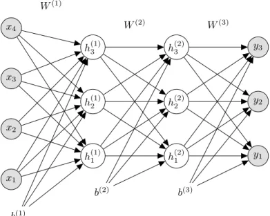
x1 x2 x3 x4 W(1) b(1) h(1)1 h(1)₂ h(1)3 W(2) b(2) h(2)1 h(2)₂ h(2)3 W(3) b(3) y1 y2 y3

Figure 2.1: A graphical representation of depth L = 3 densely connected neural network with input variables x, two hidden layers, h(1) _{and h}(2)_{, and} the output variablesy. Subscripts denote the units. In this example the input dimensionality is reduced throughout the hidden layers and the neural network outputs1-of-K classes, whereK= 3.

2.1

Supervised Learning

A deep neural network consists of a number of non-linear activation functions,

l= 1, ..., L, denoted hidden layersh(l)_{, stacked on top of each other, so that one} layer accepts the output of the layer belowh(l−1)_{as input. Each layer consists} of an activation function f(_·), and learnable parameters, weight matrix W(l)_, and bias vector b(l)_{, such thath}(l)_=f(W(l)_h(l−1)_+b(l)_{)(cf. Figure 2.1). The} activation function of the last layer L is defined differently depending on the task at hand, yˆ = g(W(L)_h(L−1)_+b(L)_{). The stacking of the neural network} layers follow:

h(0)=x, (2.1)

h(l)=f(W(l)h(l−1)+b(l)), l= 1, ..., L₋1, (2.2)

ˆ

y=g(W(L)h(L−1)+b(L)). (2.3) We refer to the combined parameter space,W(1)_{, ..., W}(L)_andb(1)_{, ..., b}(L)_asθ. As mentioned in Chapter 1, there exist multiple variants beside the one depicted

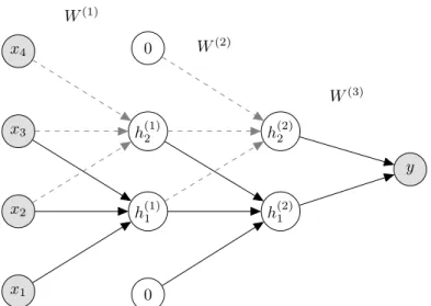
x1 x2 x3 x4 W(1) h(1)1 h(1)2 0 0 W(2) h(2)1 h(2)2 W(3) y

Figure 2.2: A graphical representation of a depth L = 3, 1D convolutional neural network with 1 channel/feature-map, input variablesx, two hidden layers,

h(1)_andh(2)_{, and the output variabley, represented by a scalar. In this example} the input dimensionality is reduced throughout the hidden layers and the neural network outputs a binary classification. The solid lines represent the kernel matrix W (we embed the bias) that is reused within the network layers. The

width of the kernel is 3 for for layers l = 1and l = 2, where the final layer is densely connected. In the first transformation we apply no padding and in the second we apply a padding of1.

in Figure 2.1. The main variants are the recurrent neural network (RNN) and convolutional neural network (CNN). This work considers the densely connected neural network and the convolutional neural network. In Figure 2.2 we give an example of a 1-dimensional convolutional neural network with only 1 channel and 1 feature map throughout the layers. The architecture is easily scaled to a 2 or 3-dimensional example with multiple feature maps that intend to capture different representations of the data. The CNN defines much fewer weights in each layer that are then shared. While lowering the amount of parameters, this triggers an ability to capture spatial structure in data.

For the neural network to learn useful representations, we must apply hidden layer activation functions f(·)that are non-linear in nature. One of the most well-known activation functions is the sigmoid function:

σ(x) = 1

1 +e−x , (2.4)

prop-erties are intriguing for optimization, as we will see later. Another well-known activation function is thetanhthat is in the range [₋1,1]:

tanh(x) = sinh(x)

cosh(x) = 2σ(2x)−1 . (2.5)

However, due to the plateaus near the limits of these activation functions, they are both prone to the phenomenon calledvanishing gradients that saturates the learning process. This is where the ReLU activation function,f(x) = max(0, x), comes handy, since it does not saturate, [0,∞]. However, it possesses the vul-nerability of activations blowing up. This can be controlled by other tricks, such as gradient clipping or batch normalization (Ioffe and Szegedy, 2015). ReLU units also result in sparse activations, because all negative values become0 (gra-dient of 0). This can come at a cost, in which many units in the neural network become passive,dying ReLU problem, which have spawn other variants, such as the leaky ReLU. The ReLU and its variants have gained tremendous traction as being the best choice for a hidden layer activation function. However, due to the properties of a bounded output interval in the case of the sigmoid and

tanh functions, they are still popular as output activation functions, g(_·). In the case of a discriminative binary classification task the activation function is a sigmoid, and a neural network with one hidden layer is given by:

ˆ

yθ(x) =σ

W(2)ReLUW(1)x+b(1)+b(2) . (2.6) Besides the binary classification task there exist two major applications within deep neural networks for supervised learning: multi-class classification and re-gression. In multi-class classification we seek to solve whether x belongs to

1-of-K classes (cf. Figure 2.1). In this case, the output activation function is denoted the softmax function and for thekth_{class, with k= 1, ..., K it is:}

softmax(ˆy)k = e ˆ yk PK j eyˆj . (2.7)

The neural network in Figure 2.1 is defined as:

ˆ

yθ(x) =softmax

W(3)ReLUW(2)ReLUW(1)x+b(1)+b(2)+b(3) .

(2.8) For continuous regression problems the output is a linear transformation. In the supervised learning problem, the aim of the learning task is to minimize the negative likelihood between the target y and the model yˆθ(x) over the

parametersθ: arg min θ − Y n pθ(yn|yˆθ(xn)). (2.9)

We often prefer to define the problem with respect to thelog-likelihood, since it (i) has the same maximum value as the likelihood, (ii) is monotonically increas-ing, and (iii) avoids overflow and underflow since multiplication and division becomes addition and subtraction in the log-space. In order to solve the opti-mization problem in Equation 2.9 we seek to define a negative log-likelihood, denoted the objective function _F(ˆyθ(x),y), that solves the task at hand. In

the binary classification task, the objective function is defined as the Bernoulli cross-entropy:

F(ˆyθ(x),y) =− X

n

(ynlog ˆyθ(xn) + (1−yn) log(1−yˆθ(xn))) , (2.10)

where yˆθ(·) is a scalar in the range [0,1]. For a multi-class classification task

the objective function is the Categorical cross-entropy:

F(ˆyθ(x),y) =− X

n

ynlog ˆyθ(xn), (2.11)

where yˆθ(·) is a vector representing 1-of-K outcomes. Since neural networks

mostly apply to complex datasets, there is often not an analytical solution to find the maximum likelihood parameter settingθM L. The problems solved with deep

neural networks are non-convex problems and the parameter space is too big to feasibly compute second-order derivatives. Therefore, we resort to a step-wise first-order derivative optimization scheme. Stochastic gradient descent (SGD) optimization proves a way to optimize the parameter w.r.t. to a mini-batch

xb and yb. This is done by first calculating the objective function F(ˆyθ(x),

and propagate this error back through each layer (backpropagation) in order to calculate the gradient_∇θF(ˆyθ(xb),yb). This process is denotedbackpropagation

(Rumelhart et al., 1986).

Optimization is performed for a predefined amount of iterations,τ, where each update is given by:

θτ+1=θτ−α∇θτF(ˆyθτ(xb),yb), (2.12)

andαis the learning rate. Compared to the gradient descent (GD) optimization scheme that updates the parameters θ for the entire dataset x, y, SGD has a regularizing effect. There exist multiple further advancements to the regular SGD optimization scheme that adapt the learning rate,α, by utilizing adaptive estimates of lower-order moments. Throughout the research we use ADAM (Kingma and Ba, 2014).

For an in-depth tutorial on neural networks, go to the lab exercises: github.com/DeepLearningDTU/02456-deep-learning Densely connected neural networks: Lab1

A thorough walk-through of the backpropagation algorithm and a guide to setup a neural network with an accompanying introduction to optimization algorithms. The tutorial also provides an introduction to neural network regularization and the reverse effect,overfitting.

Convolutional neural networks: Lab2

Introduction to the concepts of convolutional neural networks, i.e.

stride,pooling, andpadding. The lab also provides a deep understanding of the arithmetics of both the densely connected and convolutional neural network with exercises on implementing the networks without libraries such as Tensorflow (Abadi et al., 2015). It proves practical learnings from posing examples on widely used machine learning datasets.

Recurrent neural networks: Lab3

A practical introduction to recurrent neural networks. The lab provides examples on how to implement differentencoder-decoderstructured net-works with simple use-cases, such as implementing a network that maps from spelled numbers, i.e. one, two, three, to the numeric representa-tion, i.e. 1, 2, 3.

2.2

Representation learning

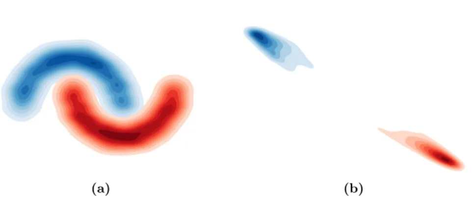
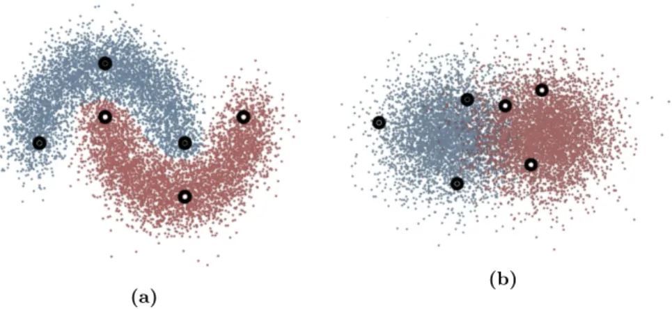
The learning process of each hidden layer throughout the neural network layers is referred to as representation learning (or feature learning), where a good representation is one that can untangle the input data distribution in order to improve on the training criterion at hand (Bengio et al., 2013). Let us consider a simple example hereof, in which we have a binary classification task consisting of twohalf-moons, where the upper half-moon belongs to the positive class and the lower half-moon to the negative class (cf. Figure 2.3). The two distributions are entangled in the input distribution and essentially impossible to discriminate between without a form of non-linearity.

Discriminating between the two half-moons is a simple task for a neural network, due to its ability to transform, i.e. rotate and resize, the data through itsW(l) matrices and perform translations through its b(l) _{vectors. This means that,}

(a) (b)

Figure 2.3: (a) Density plot of a dataset consisting of two entangled half-moons in the input space. (b) A density plot of two transformations of the two entangled half-moons, in which they have been untangled. This can be considered as a representation of the input data distribution.

by stacking multiple layers on top of each other, the neural network gets more flexible in its ability to transform and translate, hence a higher expressive power. In order to show the effect, we draw a number of examples from the distributions and apply a mesh grid to the 2-dimensional half-moon example (cf. Figure 2.4a). To make the effect more clear, we also visualize two tendency lines, one for each class. We then apply a neural network with two hidden layers, using the tanh activation function, and an output layer with the sigmoid activation function with corresponding Bernoulli cross-entropy for the purpose of binary classification (cf. Equations 2.5, 2.4, 2.10). When training the neural network, we quickly see how the input data distribution transforms and translates, by visualizing the representation in one of the hidden layers (cf. Figure 2.4b). In the end of the learning phase, where this neural network achieves an accuracy of 100%, it is evident that it has accomplished to untangle the input space, such that it is possible, for the output layer, to linearly discriminate between the two half-moons (cf. Figure 2.4c).

2.3

Unsupervised Learning

In contrast to the clear definition of supervised learning, unsupervised learning covers an extensive amount of machine learning paradigms, e.g. dimensionality reduction, clustering, anomaly detection, and generative modeling. Amongst the famous machine learning models for unsupervised learning is: principal component analysis (PCA), k-nearest neighbours (KNN),restricted Boltzmann machines (RBM), and many more. In this thesis we will limit ourselves to unsupervised learning in the context of neural network auto-encoders.

(a)

(b) (c)

Figure 2.4: Visualization of the half-moon dataset with a mesh grid in the input space (a), the beginning of training of a neural network in one of the hidden layer representations (b), and finally the visualization of the hidden representation at the end of training (c), in which the neural network is capable of discriminating between the half-moons linearly.

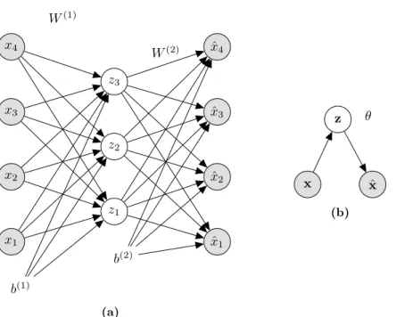
Auto means self, thus the meaning is to self-encode, which refers to having a model that can encode an inputxto a latent variablezand decode this latent variable back into the input dimension, denoted a reconstructionxˆ. In Figure 2.5a we show a simple visualization of a densely connected 1 hidden layer auto-encoder. In this context we denote the bottleneck, as a latent layer z, and the remainder of the subsequent layers (not present in this visualization) hidden layers, h. For ease of notation, we show a simpler graphical representation of the auto-encoder in Figure 2.5b, in which each edge corresponds to a stacking of hidden layers.

A breakthrough in deep auto-encoding was introduced in Hinton and Salakhut-dinov (2006). They presented a model for dimensionality reduction that applied the pre-training and fine-tuning step, from Hinton et al. (2006), to avoid vanish-ing gradients when stackvanish-ing layers. Within the pre-trainvanish-ing step, they trained RBMs with the contrastive divergence update (Hinton, 2002), which can be viewed as a 2-layer bidirectional graphical model, for each hidden layer. This pre-training method was quite cumbersome, and scaled badly when stacking many layers on top of each other. Vincent et al. (2008) introduced a simpler process for the layer-wise pre-training, denoted thedenoising auto-encoder, and later Vincent et al. (2010) complemented this with a stacked version. The intro-duction of these opened for new findings within areas such as semi-supervised learning (Ranzato and Szummer, 2008), natural image denoising (Vincent et al., 2010), topic modeling (Salakhutdinov and Hinton, 2009) and much more. In broad terms, there exist two complementary tricks to make an efficient neural network auto-encoder. One is to learn to reconstruct the input data through a bottleneck of lower dimensionality. Thisforce the model to embed the part of

x1 x2 x3 x4 W(1) b(1) z1 z2 z3 W(2) b(2) ˆ x1 ˆ x2 ˆ x3 ˆ x4 (a) x z ˆ x θ (b)

Figure 2.5: (a) A graphical representation of a densely connected auto-encoder with one hidden layer. (b) A simple graphical visualization of an auto-encoder, where the edges represent an undefined stacking of neural network layers.

the input data, from which it can reproduce it in the best way possible. The other trick, is to map from a noisy input ˜xto the reconstruction xˆ, but using the non-noisy xin the objective function,_F(ˆxθ(˜x),x).

With the advent of activation functions, such as the ReLU, and non-trivial connectivity, e.g. residual connections (He et al., 2015), the auto-encoder is not prone to the vanishing gradient problem, thus there is no need for pre-training. This has let to much more complex and expressive auto-encoder architectures such as the ladder network for semi-supervised learning (Rasmus et al., 2015) and U-Nets for image segmentation (Ronneberger et al., 2015) that can be trained in an end-to-end fashion.

For an in-depth tutorial on auto-encoders, go to the lab exercises: github.com/DeepLearningDTU/02456-deep-learning Unsupervised representation learning: Lab5

An introduction to the concept of an auto-encoder with implementation details and a walk-through on how to validate these models. The lab also contains an exercise in which the task is to build an auto-encoder for semi-supervised learning.

For an implementation of the ladder network (Rasmus et al., 2015), go to the Parmesan library:

Deep Generative Models

In this chapter we will give an introduction to a general deterministic approxi-mate inference approach calledvariational inference(Jordan et al., 1999). Next we will investigate variational inference in light of using an inference model

(Hinton and Zemel, 1993; Salakhutdinov and Larochelle, 2010) and how this approach contains caveats when estimating the gradients. Finally, we will intro-duce the variational auto-encoder (VAE) (Kingma and Welling, 2014; Rezende et al., 2014) that can be viewed as a variational inference version of the deep neural network auto-encoder, introduced in the previous chapter.

3.1

Variational Inference (VI)

As explained in Section 1.1 we can derive Bayes theorem from the likelihood

p(x_|z), theprior p(z), and the joint likelihoodp(x,z) =p(x_|z)p(z):

p(z_|x) =p(x|z)p(z) p(x) = p(x_|z)p(z) R zp(x|z)p(z)dz , (3.1)

for which p(z_|x) and p(x) is denoted the posterior and the evidence. Solving the above integral is often intractable, hence a closed form solution can not be derived. A common approach in order to solve this problem is to apply Markov Chain Monte Carlo (MCMC) techniques, in which we draw samples from the posterior, p(z|x), without knowing the normalization constant. Increasing the number of samples drawn will ensure that the expectation converges towards the true posterior. We will not go into the different MCMC techniques here, but common features are, that they will eventually converge to the truep(z|x), but have a tendency to be cumbersome in regards to training and convergence time for a high-dimensionalz-space (latent space). In many applications the use of a too simple low dimensional latent space introduces a lack of expressiveness when modeling complex input data distributions. This can be related to the bottleneck of the neural network auto-encoder. If this is too low-dimensional, it is impossible to reconstruct the data sufficiently.

Variational inference (VI) is an approach in which we optimize the parameters,

φ, of avariational approximation,qφ(z), that approximates the posterior, so that

qφ(z)≈p(z|x). In the following paragraphs, for the sake of simplicity, we will

refer to the posterior and the variational approximation as discrete distributions,

P(z|x)andQφ(z).

In order to explain VI in more details, we first introduce the notion ofentropy. If we draw a sample from the discrete probability distribution, P(z|x), the entropy of this specific draw will be high as a function of how improbable it is. Conversely, if a specific draw fromP(z_|x)is the same every time, then the entropy is 0. From an information theoretical view, the entropy describes the average amount of information that is transfered from a sender to a receiver

w.r.t. toP(z_|x). The entropy of a random variablezcan be seen as thedegree of surprise for an event to happen (Bishop, 2006) and is defined as:

H(P(z_|x)) =_EP(z|x)[−logP(z|x)] =−

X z

P(z_|x) logP(z_|x). (3.2) Now that we have a notion of the entropy, we are interested in a measure that describes a similarity between our variational approximation, Qφ(z), and the

does that by describing the amount of additional information needed if a sender transmits z to a receiver through Qφ(z) rather than P(z|x). In other words

it provides a measure to determine the difference between a distributionQφ(z)

andP(z_|x). It is defined as:

DKL[P(z|x)||Qφ(z)] =− X z P(z_|x) log Qφ(z) P(z|x) = X z P(z_|x) logP(z|x) Qφ(z) . (3.3) It is important to note thatDKL(·)is not symmetrical,DKL[P(z|x)||Qφ(z)]6=

DKL[Qφ(z)||P(z|x)]. It is also easily shown that the cross-entropy loss

(intro-duced in Equation 2.11) derives from exactly_H(P(z_|x))andDKL[P(z|x)||Qφ(z)]:

H(P(z|x), Qφ(z)) =H(P(z|x)) +DKL[P(z|x)||Qφ(z)] =₋X z P(z_|x) logP(z_|x)₋X z P(z_|x) log Qφ(z) P(z|x) =−X z P(z|x) logP(z|x)Qφ(z) P(z|x) =₋X z P(z_|x) logQφ(z). (3.4)

DKL(·)is easily extended to continuous distributionsp(z|x)andqφ(z):

DKL[p(z|x)||qφ(z)] =− Z

z

p(z_|x) log qφ(z)

p(z_|x)dz . (3.5)

Furthermore a property, is that DKL(·)≥0, which can be shown by utilizing Jensen’s inequality1_: DKL[qφ(z)||pθ(z|x)] =− Z z qφ(z) log pθ(z|x) qφ(z) dz ≥ −log Z x qφ(z) pθ(z|x) qφ(z) dx =−log Z x pθ(z|x)dx=−log 1 = 0. (3.6)

In order to solve the problem from Equation 3.1, we introduce parameters θ

for the joint distribution pθ(x,z). We seek to find an approximation to the

intractable part of the theorem,p(x) =R_zp(x,z)dz, such that:

arg max θ N Y i pθ(xi). (3.7)

The objective function for the optimization problem is normally derived di-rectly from the evidence, however we intend to derive it slightly differently. As stated above, we introduce the variational approximation with parameters φ, and require that it must be similar to the posterior. In order to define this relationship, we can apply the KL-divergence to the two distributions. Hence, when the KL-divergence is small, we ensure thatqφ(z)≈p(z|x). However, due

to the asymmetry, we must define whether we deploy theforward KL-divergence

DKL[pθ(z|x)||qφ(z)]or thereverseKL-divergenceDKL[qφ(z)||pθ(z|x)]. Murphy

(2012) amongst others, notice that there is properties that may affect an opti-mization problem when defining one over the other. Ifqφ(z) = 0andpθ(z|x)>0

the forward KL-divergence is infinite, referred to as zero avoiding. The result of this is thatqφ(z)has a tendency to overestimate the support ofpθ(z|x). The

reverse KL-divergence on the other hand is infinite forpθ(z|x) = 0andqφ(z)>0

(zero forcing), which results in a tendency whereqφ(z)underestimatespθ(z|x).

In order to exemplify the result of using one over the other, it is helpful to imaginepθ(z|x)as a bimodal distribution andqφ(z)as a unimodal distribution.

Optimizing w.r.t. the forward KL-divergence will result in the unimodal dis-tribution covering the full support of the bimodal disdis-tribution. However, this comes at a cost, since there will be many regions covered byqφ(z)with no

den-sity forpθ(z|x). Conversely, the reverse KL-divergence would fit the unimodal

distribution to one of the modes of the bimodal distribution and would thereby be an underestimation of the true posterior. In order to avoid that the distri-bution qφ(z)covers too many no-density regions we derive the objective of the

optimization problem from the reverse KL-divergence:

DKL[qφ(z)||pθ(z|x)] =− Z z qφ(z) log pθ(z|x) qφ(z) dz. (3.8)

Another reason for starting with the reverse KL-divergence is that taking the expectation,R_zqφ(z) =Eqφ(z) is tractable compared to the opposite. However, the above does not suffice, since it is only defined w.r.t. the posterior. Referring back to Bayes theorem, we need to optimize for the joint probability pθ(x,z).

Introducing the evidence to the above can easily embed this:

DKL[qφ(z)||pθ(z|x)] =− Z z qφ(z) log pθ(x) pθ(x) pθ(z|x) qφ(z) dz =₋ Z z qφ(z) log pθ(z,x) qφ(z)pθ(x) dz =₋ Z z qφ(z) log pθ(z,x) qφ(z) dz+ logpθ(x). (3.9)

As explained earlier, it is intractable to optimize w.r.t. the evidence, so Equation 3.9 can be rearranged: logpθ(x) =DKL[qφ(z)||p(z|x)] + Z z qφ(z) logpθ(z,x) qφ(z) dz. (3.10)

From the above we have achieved to isolate the evidence (normalization con-stant). However, we are still dependent on the reverse KL-divergence. Since we know thatDKL≥0, we can remove this term from Equation 3.10 resulting in a

lower bound on the evidence, denotedevidence lower bound (ELBO) for which there is no dependency on the true posterior:

logpθ(x)≥ Z z qφ(z) logpθ(x|z)pθ(z) qφ(z) dz =Eqφ(z)[logpθ(x|z)]−DKL[qφ(z)||pθ(z)]≡ Lφ,θ(x). (3.11)

We now have an optimization problem and we can optimize the bound w.r.t.

φ and θ where at the maximum value, the variational approximation equals the posterior, qφ(z) = p(z|x), and the bound equals the evidence, Lφ,θ(x) = logpθ(x). The integral in the ELBO does not naturally introduce less

com-plexity. However, since we have replaced the dependency on p(z_|x) with one onqφ(z), we now have the option to choose from a tractable family, for which

we can achieve a good approximation to the posterior and one where we can optimize the parametersφefficiently.

3.2

VI with Deep Neural Networks

For high-dimensional complex datasets, e.g. images our audio, it will not suf-fice to introduce qφ(z)as a simple tractable distribution. We need to somehow

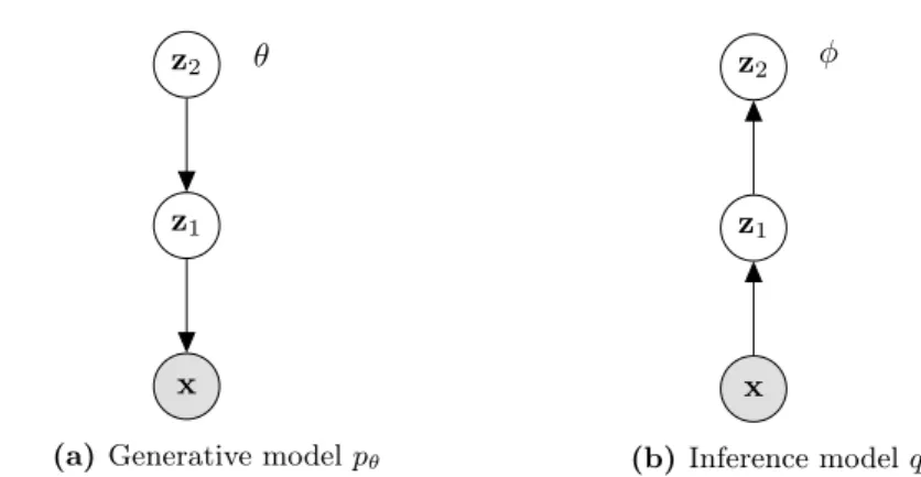
approximate the posterior through an expressive model. This is denoted an in-ference model for which we have seen many different parameterizations through time (Hinton and Zemel, 1993; Dayan and Hinton, 1996; Salakhutdinov and Larochelle, 2010). In Figure 3.1 we present a graphical representation of a prob-abilistic model with a latent variablezand observed variablex. The generative model is factorized as pθ(x,z) =pθ(x|z)pθ(z)and the corresponding inference

model isqφ(z|x). Parameterizing the inference and generative models with

neu-ral networks provide a more expressive model, since the deep neuneu-ral network can find a non-linear representation that lies on a manifold within a tractable distribution. However, as we shall see, using a deep neural network inference model raises problems during optimization, due to high variance of the gradient estimates.

x

z θ

(a) Generative modelpθ

x

z φ

(b)Inference modelqφ

Figure 3.1: Graphical representation of the generative model parameterized by θ (a) and the variational approximation/inference model parameterized by

φ(b). zrepresents a latent variable that can either be expressed by a discrete or continuous distribution andxrepresents the observed variable.

3.2.1

A High-Variance Gradient Estimator

In order to formulate a gradient estimator for these models, we must first derive the ELBO from Equation 3.11 w.r.t. θ:

∇θL(x) =∇θ Z z qφ(z|x) logpθ(x,z)dz− ∇θ Z z qφ(z|x) logqφ(z|x)dz = Z z qφ(z|x)∇θlogpθ(x,z)dz =_Eqφ(z|x)[∇θlogpθ(x,z)] . (3.12)

Thezfor calculating the gradient w.r.t. θis thereby dependent on a sample from the variational approximation. Since the ELBO is dependent on the expectation over the variational approximation, which is a function ofφ, the gradients w.r.t. toφis calculated in a slightly different way:

∇φL(x) =∇φ Z z qφ(z|x) logpθ(x,z)dz | {z } ∇φLA(x) − ∇φ Z z qφ(z|x) logqφ(z|x)dz | {z } ∇φLB(x) . (3.13)

We split the gradient w.r.t. φinto two terms for convenience, for which the first term is given by:

∇φLA(x) =∇φ Z z qφ(z|x) logpθ(x,z)dz = Z z∇ φqφ(z|x) logpθ(x,z)dz. (3.14)

The derivation of the second term is a little more complex, since we must deploy the product rule for gradients2_{, and the chain rule on thelog-likelihood}3_:

∇φLB(x) =∇φ Z z qφ(z|x) logqφ(z|x)dz = Z z qφ(z|x)∇φlogqφ(z|x)dz+ Z z∇ φqφ(z|x) logqφ(z|x)dz = Z z qφ(z|x) ∇φqφ(z|x) qφ(z|x) dz+ Z z∇ φqφ(z|x) logqφ(z|x)dz =_∇φ Z z qφ(z|x)dz+ Z z∇ φqφ(z|x) logqφ(z|x)dz =_∇φ1 + Z z∇ φqφ(z|x) logqφ(z|x)dz = Z z∇ φqφ(z|x) logqφ(z|x)dz. (3.15)

From knowing that_∇φqφ(z|x) logqφ(z|x) =qφ(z|x)∇φlogqφ(z|x)we can

com-bine the two terms by:

∇φL(x) =∇φLA(x)− ∇φLB(x) = Z z∇ φqφ(z|x) logpθ(x,z)dz− Z z∇ φqφ(z|x) logqφ(z|x)dz = Z z∇ φqφ(z|x) [logpθ(x,z)−logqφ(z|x)]dz = Z z

qφ(z|x)∇φlogqφ(z|x) [logpθ(x,z)−logqφ(z|x)]dz =Eqφ(z|x) logpθ(x,z) qφ(z|x)∇ φlogqφ(z|x) . (3.16)

In order to calculate the gradients in Equation 3.12 and 3.16 we apply Monte Carlo integration over a number of samples sto estimate:

∇θL(x)≈ 1 s s X i=1 Eqφ(z(i)_|x) h ∇θlogpθ(x,z(i)) i , (3.17) and ∇φL(x)≈ 1 s s X i=1 Eqφ(z(i)_|x) logpθ(x,z (i)₎ qφ(z(i)|x)∇φ logqφ(z(i)|x) . (3.18) 2_{∇(f·g) =∇f·g+f· ∇g} 3_{∇logp(x) =∇p(x)/p(x)}

By utilizing the MCMC gradient estimators it is straightforward to apply a SGD algorithm to optimize the parameters φ and θ. However, due to the scaling-term of the gradients w.r.t. φinside the expectation,E_qφ(z(i)_|x)[·], the estimator

in Equation 3.18 has proven close to useless (Mnih and Gregor, 2014; Hinton and Zemel, 1993; Dayan and Hinton, 1996). To circumvent the issue of high-variance gradient estimates, Mnih and Gregor (2014) introduced a technique to reduce variance, denoted neural variational inference and learning (NVIL), by applying control variates. Another less general, but more popular, approach to estimate the gradients of a generative model and inference model is to apply the

reparameterization trick (Kingma and Welling, 2014; Rezende et al., 2014).

3.2.2

Variational Auto-Encoder

Instead of assuming thatz(i)

≈qφ(z(i)|x), the reparameterization trick changes

the variablez(i) _{to come from a deterministic function:}

z(i)=gφ((i),x), (3.19)

where (i)

≈ p((i)_{). The gradients w.r.t. φ are hereby not dependent on the} expectation and this results in a much simpler formulation of the gradient esti-mator: ∇φ,θL(x)≈ 1 s s X i=1 Ep((i)₎ ∇φ,θlog pθ(x, gφ((i),x)) qφ(gφ((i),x)|x) . (3.20)

With the above formulation, the gradient is not dependent on stochasticity in the generative and inference model, thus the entire modelθandφis differential w.r.t. to the ELBO. This means that we can now backpropagate the ELBO through the generative model θ followed by the inference model φ, which is prone to much less variance, due to the elimination of the disjoint update. Furthermore, it is easily implemented in modern frameworks, e.g. Tensorflow (Abadi et al., 2015) that utilize automatic differentiation. A model that applies the reparameterization trick, while being parameterized by neural networks in both generative and inference models, is often referred to as avariational auto-encoder (VAE) (cf. Figure 3.2) (Kingma and Welling, 2014; Rezende et al., 2014), due to its obvious similarity with the neural network auto-encoder. The reparameterization trick applies to a wide family of continuous latent vari-ables, but the Gaussian is the most common, for which the trick is given by:

The generative model of the most commonly used VAE is thereby decomposed by: pθ(x,z) =pθ(x|z)pθ(z), (3.22) with pθ(z) =N(z|0, I) (3.23) pθ(x|z) =N(x|µθ(z), σθ(z)) or Pθ(x|z) =B(x|µθ(z)), (3.24)

where _N(_·)and_B(_·)denote the Gaussian and Bernoulli distribution. The cor-responding inference model is given by:

qφ(z|x) =N(z|µφ(x), σφ(x)). (3.25)

µφ(x),σφ(x),µθ(z), σθ(z)are all parameterized by deep neural networks. The

inference model is thereby defined as:

h(0)=x, (3.26) h(m)_=f(W(m)_h(m−1)_+b(m)_{), m= 1, ..., M} −1, (3.27) µφ=Wφ,µ(M)h(M−1)+b (M) φ,µ, (3.28) σφ=softplus(Wφ,σ(M)h(M−1)+b (M) φ,σ), (3.29)

wheresoftplus denotes an activation function with similar characteristics as the ReLU, while being differentiable in 0. After defining each element of the VAE it becomes obvious that the two terms in Equation 3.11 can be viewed as a reconstruction regularized by a term that keeps the variational approximation close to the uninformative prior:

Lφ,θ(x) =Eqφ(z)[logpθ(x|z)] | {z } reconstruction term −DKL[qφ(z|x)||pθ(z)] | {z } regularization term . (3.30)

When DKL[qφ(z)||pθ(z)] = 0 there will be no information going from the en-coder. This will be referred to as the latent variable zis collapsing and will be discussed further in Section 3.3.

From the above formulation of the typical VAE it is obvious that rather limiting assumptions are made on the true posterior distribution p(z|x). First of, it is assumed that the posterior distribution is factorial, so that all variables are statistically independent, p(x1, x2) = p(x1)p(x2). Another assumption is that the neural networks, used in the inference and generative models, are flexible

enough to map complex input distributions p(x) into a rather simple qφ(z|x)

Burda et al. (2015) was among the first to identify this problem. They pro-posed theimportance-weighted auto-encoder(IWAE), which is a way to perform multiple samples in the variational approximation, qφ(z|x), so that the ELBO

becomes tighter and the model performs a better approximation towards the true posterior. In their work an unbiased estimator of p(x) is introduced that applies importance weights inside thelog-term of Equation 3.30:

Lφ,θ(x) =Eqφ(z|x)  log1 k k X j=1 pθ(x|z(j))pθ(z(j)) qφ(z(j)|x)   . (3.31)

The intuition behind Equation 3.31 is that the normal VAE emphasizes high-probability regions of the approximate posterior too much, leaving little to low-probability regions. In the IWAE we loosen the restrictions such that the vari-ational approximation may fit a true posterior that does not align with the limiting assumptions of the VAE. Note that the 1-sample IWAE is equivalent to the standard VAE. In this thesis we will refer to the ELBO of a VAE as formulated in Equation 3.31, where we omit the parameters φ andθ for short and_L(x)denotes 1 IW sample and_L10(x)denotes 10 IW samples.

Despite the significant improvement from using the tighter bound in equation 3.31 compared to Equation 3.11 the single latent layer with a relatively simple distribution still pose a limiting constraint to approximate the true posterior. There are two main research paths that intend to solve this problem, by (i) adding more latent variables, and (ii) modeling a more flexible distribution for each latent variable. The research throughout this thesis mainly concerns (i), where it is important to note that most of the findings in (i) and (ii) are not mutually exclusive.

For an in-depth tutorial on variational auto-encoders, go to the lab exercises:

github.com/DeepLearningDTU/02456-deep-learning Variational auto-encoders: Lab5

An introduction to the derivation and theoretical background of the variational auto-encoder in cohesion with a Tensorflow (Abadi et al., 2015) implementation on how to implement and train a one latent layer model.

For an implementation of the importance weighted auto-encoder (Burda et al., 2015), go to the Parmesan library:

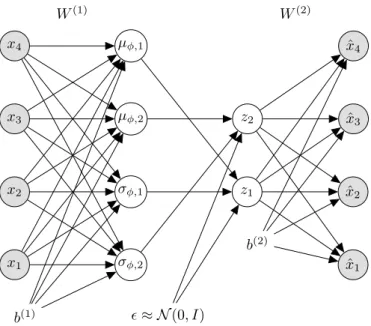
x1 x2 x3 x4 W(1) b(1) σφ,2 σφ,1 µφ,2 µφ,1 _{≈ N}(0, I) z1 z2 b(2) ˆ x1 ˆ x2 ˆ x3 ˆ x4 W(2)

Figure 3.2: Visualization of a densely connected variational auto-encoder (VAE) with one latent layerzconsisting of two units and no hidden deterministic layers. From this visualization it is evident that the VAE enables backpropa-gation through all variables, since the stochastic variable can be circumvented when applying the chain-rule.

3.3

Towards a Richer Posterior

This section cites two of the contributions in this thesis:

B Sønderby, C.K., Raiko, T., Maaløe, L., Sønderby, S. K., Winther, O.. Ladder variational autoencoders. In Advances in Neural In-formation Processing Systems, pages 3738-3746.

C Maaløe, L., Fraccaro, M., Winther, O. (2017). CaGeM: A cluster aware deep generative model. In Neural Information Processing Systems Workshop on Approximate Bayesian Inference.

The general assumption is to formulate the VAE with a diagonal covariance, which leaves limitations to the expressiveness of the model, since qφ(z|x) will

be restricted in modeling more complex posteriors. Hence, if the data lies on a complex posterior, the variational approximation could be a bad fit. Adding more latent layers may improve flexibility, since the model is thereby able to learn different representations of the posterior throughout the latent variables.

x z1

z2 θ

(a) Generative modelpθ

x z1

z2 φ

(b)Inference modelqφ

Figure 3.3: Graphical representation of the generative model parameterized by θ (a) and the variational approximation/inference model parameterized by

φ (b) for a two latent layer hierarchical VAE. z1 and z2 represent the latent variables expressed by continuous distributions and x represents the observed variable.

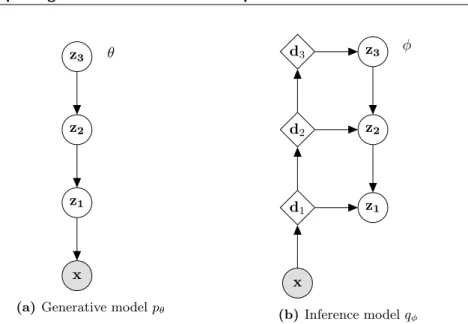
This leads to the more general formulation of the VAE withLlatent layers (cf. Figure 3.3): pθ(x,Z) =pθ(x|z1)pθ(zL) L_Y−1 i=1 pθ(zi|zi+1), (3.32) whereZ=zi, ...,zL and: pθ(zi|zi+1) =N(zi|µθ,i(zi+1), σθ,i(zi+1)), pθ(zL) =N(zL|0, I) (3.33) pθ(x|z1) =N(x|µθ,0(z1), σθ,0(z1)) or Pθ(x|z1) =B(x|µθ,0(z1)). (3.34) The correspondingvanillainference model is decomposed by:

qφ(Z|x) =qφ(z1|x) L Y i=2 qφ(zi|zi−1), (3.35) with qφ(z1|x) =N(z1|µφ,0(x), σφ,0(x)), qφ(zi|zi−1) =N(zi|µφ,i(zi−1), σφ,i(zi−1)). (3.36)

The reason why a model with more latent layers may introduce more flexibility is simply that it has more expressive power through the ability to learn multiple representations of the approximation to the posterior. The view on representa-tion learning introduced in Secrepresenta-tion 2.2 is especially useful here. Thus, in many

settings of hierarchical VAEs we seek to introduce dimensionality reduction be-tween each latent layerz1, ...,zL, such that we force the network to learn more

and more global information of the data distributionp(x). Another intriguing property of the above formulation is that the latent layersz1, ...,zL−1are more flexible, since the prior is learned as opposed to that of pθ(zL) =N(zL|0, I).

Finally, the hierarchical VAE introduces an intuitively compelling feature dur-ing inference (traindur-ing), which bears resemblance to finddur-ings in the purely de-terministic neural networks. Throughout the recent research within deep neural networks, we have seen many research contributions that successfully apply very deep architectures without the network being prone to vanishing gradi-ents. These contributions mainly concern skip-connectivity, such as residual connections (He et al., 2015),highway networks (Srivastava et al., 2015), and

densely connected networks (Huang et al., 2017). These inventions have been successful in very deep auto-encoder architectures, such as the PixelCNN++ (Salimans et al., 2017) and U-Net (Ronneberger et al., 2015). The intention of the skip-connectivity is to keep the path from the input to the output of the neural network as short as possible, while still having a deep stacking of layers that can learn highly non-linear representations. The skip-connections ensure that the inference-signal can skip the subsequent layers. During inference of the VAE, each latent variable can be viewed as a skip-connection between the infer-ence model and the generative model. This is due to the fact that the sample

z1 ≈ qφ(z1|x) serves as input to pθ(x|z1) and z2 ≈ qφ(z2|z1) serves as input topθ(z1|z2)and so forth. For a very deep hierarchical inference and generative model we can thereby utilize thenatural skip-connectivity in order to learn very deep architectures.

However, as presented in Sønderby et al. (2016) (see Appendix B) among others, the latent layers have a tendency to collapse whenL >2. Maaløe et al. (2017) (seeAppendix C) gives an explanation to this problem in which we first consider the asymptotic average properties by taking the expectation over the true evidence of the data distributionpd(x). This is applied to thelog-likelihood

of model pθ(x)(cf. Equation 3.2, 3.3, 3.4): Epd(x)[logpθ(x)] = Z x pd(x) logpθ(x)dx = Z x pd(x) logpd(x)pθ(x) pd(x) dx = Z x pd(x) logpd(x) + Z x pd(x) log pθ(x) pd(x) dx =−H(pd(x))−DKL[pd(x)||pθ(x)] . (3.37)

Thus, the expectedlog-likelihood is the difference between the negative entropy of the data generating distribution pdata(x), and the deviation between the

data generating distributionpd(x)and the model distributionpθ(x). When we

introduce a latent variable to the model, such that pθ(x) = R_zpθ(x|z)pθ(z)dz

we can derive the ELBO by:

logpθ(x) = log Z z pθ(x,z)dz = log Z z qφ(z|x) qφ(z|x) pθ(x,z)dz ≥ Z z qφ(z|x) log pθ(x,z) qφ(z|x) dz =_Eqφ(z|x) logpθ(x,z) qφ(z|x) . (3.38)

We will now take the expectation over the true evidence of the data distribution on our new model:

Epd(x)[logpθ(x)]≥Epd(x) Eqφ(z|x) logpθ(x,z) qφ(z|x) = Z x pd(x) Z z qφ(z|x) log pθ(x,z) qφ(z|x) dzdx = Z x pd(x) Z z qφ(z|x) logpd(x) pθ(x) pd(x)− logpθ(z|x) qφ(z|x) dzdx = Z x pd(x) logpd(x) pθ(x) pd(x) dx₋ Z x pd(x) Z z qφ(z|x) log pθ(z|x) qφ(z|x) dzdx =_−H(pd(x))−DKL[pd(x)||pθ(x)]−Epd(x)[DKL[qφ(z|x)||pθ(z|x)]] . (3.39) When comparing Equation 3.37 with Equation 3.39 it is obvious that adding a latent variable z will add additional cost. Hence, the model has an in-centive to omit the latent variable during optimization, which may eventu-ally result in a collapse. Conversely, if the introduced latent variable proofs beneficial in maximizing the log-likelihood beyond the additional cost it will not collapse. It is trivial to show that the cost of adding more variables is even higher. Following the same derivation as in 3.39 for a model, pθ(x) = R z1,z2pθ(x|z1)pθ(z1|z2)pθ(z2)dz1dz2we get: Epd(x)[logpθ(x)]≥ −H(pd(x))−DKL[pd(x)||pθ(x)] −Epd(x)[DKL[qφ(z1|x)||pθ(z1|x)]] −Epd(x)[DKL[qφ(z2|z1)||pθ(z2|z1)]] . (3.40) Since we initialize the variational approximation with deep neural networks, the samples from the latent variables will be very noisy in the beginning of a

SGD optimization. Therefore, the model will have a larger incentive to collapse latent variables in the beginning of training, resulting in a poor local maxima. As stated in Bowman et al. (2016); Fraccaro et al. (2016); Chen et al. (2017) the collapse of latent variable can also happen when the decoder neural network, parameterized byθ, is very powerful. In the following chapters we will elaborate more on our findings concerning how to avoid latent variables to collapse in deep generative models.

Concluding remarks There still remains a lot of recent research, that is not included in this thesis, investigating a more expressive VAE framework, such as inverse autoregressive flows (IAF) (Kingma et al., 2016), variational inference withnormalizing flows(Rezende and Mohamed, 2015), and variational Gaussian processes (Tran et al., 2016). There are also variants of using the reparameterization in a supervised learning paradigm by applying priors to the weights of a neural network (Blundell et al., 2015).