Stronger together: Multi-annual variability of hydrogen production supported by wind power in Sweden

Applied Energy 282 (2021) 116082

Available online 19 November 2020

0306-2619/© 2020 The Authors. Published by Elsevier Ltd. This is an open access article under the CC BY license (http://creativecommons.org/licenses/by/4.0/). Contents lists available atScienceDirect

Applied Energy

journal homepage:www.elsevier.com/locate/apenergy

Stronger together: Multi-annual variability of hydrogen production

supported by wind power in Sweden

Christian Mikovits

_{, Elisabeth Wetterlund}

, Sebastian Wehrle

_{, Johann Baumgartner}

_,

Johannes Schmidt

a_{Institute for Sustainable Economic Development, University of Natural Resources and Life Science, Vienna, Austria} b_{Energy Engineering, Division of Energy Science, Luleå University of Technology, 971 87 Luleå, Sweden} c_{International Institute for Applied Systems Analysis (IIASA), A-2361 Laxenburg, Austria}

A R T I C L E

I N F O

A B S T R A C T

Hydrogen produced from renewable electricity will play an important role in deep decarbonisation of industry. However, adding large electrolyser capacities to a low-carbon electricity system also increases the need for additional electricity generation from variable renewable energies. This will require hydrogen production to be variable unless other sources provide sufficient flexibility. Existing sources of flexibility in hydro-thermal systems are hydropower and thermal generation, which are both associated with sustainability concerns. In this work, we use a dispatch model for the case of Sweden to assess the power system operation with large-scale electrolysers, assuming that additional wind power generation matches the electricity demand of hydrogen production on average. We evaluate different scenarios for restricting the flexibility of hydropower and thermal generation and include 29 different weather years to test the impact of variable weather regimes. We show that (a) in all scenarios electrolyser utilisation is above 60% on average, (b) the inter-annual variability of hydrogen production is substantial if thermal power is not dispatched for electrolysis, and (c) this problem is aggravated if hydropower flexibility is also restricted. Therefore, either long-term storage of hydrogen or backup hydrogen sources may be necessary to guarantee continuous hydrogen flows. Large-scale dispatch of electrolysis capacity supported by wind power makes the system more stable, if electrolysers ramp down in rare hours of extreme events with low renewable generation. The need for additional backup capacities in a fully renewable electricity system will thus be reduced if wind power and electrolyser operation are combined in the system.

1. Introduction

Hydrogen is considered as one crucial option for deep decarbon-isation of energy and industrial sectors, in particular in the fields of transportation [1], as feedstock for fuel or chemical production, as a reductant in primary steelmaking [2], or as energy storage in stationary heat [3] and electricity [4] applications. Today, natural gas constitutes the primary source for hydrogen production [5]. However, to allow for an actual contribution to decarbonisation, hydrogen has to be gener-ated in a carbon-free way. The electrolysis of water, using carbon-free renewable electricity, is one potential technological pathway.

Significant additional amounts of renewable electricity generation have to come, however, from intermittent generation such as solar PV or wind power, i.e., variable renewable generation (VRE), at least in regions that already use their hydropower up to its full potential.

∗ _{Corresponding author at: Energy Engineering, Division of Energy Science, Luleå University of Technology, 971 87 Luleå, Sweden.}

E-mail addresses: [email protected](C. Mikovits),[email protected](E. Wetterlund),[email protected](S. Wehrle), [email protected](J. Baumgartner),[email protected](J. Schmidt).

In effect, the need for additional flexibility is set to increase in the absence of additional measures. Operating electrolysers in a variable way to align with the renewables’ variability is possible in principle. Nevertheless, due to their high investment cost, the economics of elec-trolysers demand high utilisation rates, and ‘peak shaving’, i.e., using electrolysers to produce hydrogen from limited peaks in intermittent generation, is therefore economically not competitive [6]. Also, the quantities of hydrogen produced would be relatively small if only otherwise curtailed electricity is used.

Attaining a high utilisation rate of electrolysers under high VRE penetration therefore may increase the need for other flexibility options in the system. Hydro-thermal systems, such as our Swedish case study system, offer already significant flexibility today as both hydropower with storage and thermal generation can adapt their output according to system demands.

https://doi.org/10.1016/j.apenergy.2020.116082

Hydropower dominated systems can offer flexibility on all time scales, from hours [7] to seasons to years [8]. The highly flexible operation of hydropower plants for system integration of VRE, how-ever, causes increased rapid sub-daily fluctuations in water flow and water levels (hydropeaking). This conflicts with other environmental quality objectives as short-term river regime alteration poses a critical threat to river ecosystems [9,10], further increasing already present negative impacts of hydropower generation [11]. The negative impacts of higher penetration of renewables on hydropeaking have indeed been assessed before for past periods [12] and in modelling studies for future renewable energy systems [13].

Using thermal power generation more flexibly has minor conse-quences in terms of lower efficiency of thermal power plants in part-load operation [14]. However, depending on the system setup, thermal generation may even increase if used to guarantee a high utilisation rate for electrolysers. This comes at the cost of increased usage of fuels and associated air pollution impacts [15] and CO2-emissions. The increased use of biomass as an alternative to fossil fuels also has its environmental risks [16] and is limited by the sustainable sourcing potential. Thermal power generation should, therefore, be limited.

Previous work has widely investigated the role of electrolysis-based hydrogen in energy and electricity systems, and several recent reviews show the vital role of hydrogen in a future decarbonised energy world as it is tradable [17], and as it is crucial to decarbonise some industries and modes of transportation [3]. In particular, electrolysers have been shown to allow for higher shares of renewables in power systems, in for example Europe [18], a sub-region in Norway [19], and California [20]. Hydrogen storage has also been shown to mitigate the problem of hydro-peaking [21] and to lower the spilling of water in hydropower cascades [22]. Most studies have assumed that hydrogen production operates on surplus renewable electricity. Robinius et al. [23] assessed surplus electricity at high resolution and studied how it can be used for transport purposes in Germany. In a more detailed regional analysis, Robinius et al. [24] investigated the use of hydrogen production to prevent grid expansion. McKenna et al. [6] assessed the use of resid-ual renewable power generation for synthetic natural gas production, which could be fed to the natural gas grid for a German region. In contrast, Bolívar Jaramillo and Weidlich [25] showed that an electrol-yser under optimal conditions will not necessarily be limited to using excess power, but can be used to limit the peak power drawn from the grid. Their analysis, however, was limited to a small micro-grid system. Recently, Brey [26] analysed the Spanish power system and concluded that, apart from being used as means to store excess electricity, hy-drogen is important for the seasonal balancing of renewable supply and electricity demand. A limited amount of studies have assessed the production profile of renewable hydrogen production, either with a global approach [27] or nationally for the case of Australia [28]. None of the studies, however, assessed (1) how annual climatic variations impact the long-term variability of hydrogen output, (2) how existing flexibility measures in hydro-thermal systems can be used to stabilise hydrogen generation, (3) how the interplay of these flexibility measures affects the hydrogen output of electrolysers, and (4) how the need for backup capacities in the system is affected by introducing electrolysers and wind power.

We assess these open questions for the case of Sweden, assuming that additional electricity for electrolysis comes from wind power only. We study the system by gradually restricting the flexibility of hy-dropower and thermal power generation and observing the utilisation rate of electrolysers and the development of other system parameters, such as requirements for backup capacities.

We chose Sweden as a case to study as the country is well-positioned to take a lead in the production of low-carbon hydrogen. Sweden has a power system with a minimal CO2-emission footprint, and strong policies in place to support full decarbonisation, including a goal of 100% renewable electricity production by 2040 [29]. The above-mentioned trade-off between increased hydropower production to meet

future needs in the energy system and reduced environmental impact on rivers is evident in the Swedish system [30], and hydropeaking has been observed as both high and increasing in Nordic regulated rivers [12,31]. Hydrogen is also being outlined as a potential key technology in the future Swedish energy system, both as a flexibility technology to balance a high VRE share in the power system, for production of biofuels, and as a reductant in the steel industry, where hydrogen is currently considered as the main track for decarbonisation of primary steelmaking in Sweden [32]. While the results of our case study cannot be quantitatively transferred to other world regions, our qualitative conclusions do apply to other hydro-thermal systems with hydropower shares larger than 35%, such as Brazil, Canada, New Zealand, or Austria [33] as well.

Hydropower dominated electricity systems are prone to large inter-annual variations in water availability, as shown for Brazil [34] and Sweden [35]. To a limited extent, wind power systems also show inter-annual variability [36]. A multi-year approach to assessing energy systems with high shares of renewables is, therefore, necessary [37]. In order to be able to capture inter-annual variations and extreme weather events realistically, we use simulations of time series of VRE and electricity demand in a dispatch model for the Swedish power system for 29 different weather years, at hourly temporal resolution. We can thus assess how both short-term (hours to days) and long-term (days to months to years) variability of climatic variables drive power production patterns. The model was developed by Höltinger et al. [35], and we extend it to allow simulation of electrolyser tech-nology and a more detailed representation of thermal power generation and hydropower operational restrictions.

2. Material and methods

We assess here how different scenarios of thermal and hydropower flexibility affect the utilisation of electrolysers using a generation dis-patch model for our case study of Sweden. Our model is rooted in a well-established tradition of power system models, such as ELMOD [38], EMMA [39], REMix [40], or PyPSA [41]. In line with this, Höltinger et al. [35] have developed a power system model that is fit for its purpose. That is, the model reflects the specifics of the Swedish power system at a temporal granularity suitable for the representation of the variability of renewable electricity generation, while still being computationally tractable. We have extended and refined the model further, to ensure its appropriateness for our analysis.

In the following section, we present the general model structure and most relevant parts, as well as the major changes compared to the work by Höltinger et al. [35], with a more comprehensive and detailed model description given inAppendix A.1. The optimisation program (written inGAMSand controlled byPython), the data necessary to run the simulations, the results of the simulations, and theRCode for result analysis can be found on Zenodo [42].

2.1. Dispatch model and data 2.1.1. Model description

The optimisation model is based on hourly data for natural river runoff, load, and wind generation and aims to minimise the total vari-able system cost less the revenue from hydrogen production. Residual demand, i.e., the mismatch of wind power generation and load, has to be balanced by thermal and hydropower plants, and by the curtailment of wind power. Potential further balancing needs are provided from further backup measures. These backup measures were assumed to be available at low investment but high variable costs, as they are used with low frequency. Potential candidate technologies were additional thermal peaking plants, demand-side management measures, or im-ports from neighbouring countries. These were, however, not modelled in detail.

To be able to account for climate variability, we ran the model for 29 different weather years, which were used to simulate temperature-dependent load, hydropower, andwind power generation in the model. The model optimises a single year of dispatch, i.e. inter-annual water storage was not considered.

A temperature-dependent load profile of electricity demand was de-rived from a regression model based on reanalysis temperature data for 29 years and gridded population raster data (for details, see Höltinger et al. [35]). The modelled annual load on average equalled the average annual observed load in the period 2010–2018 (approximately 130 TWh𝑎−1, excluding transmission losses). We also considered increased power demand from electrolysis (see Section 2.2.1), but not from other uses such as increased demand by industry, data-centres, or electrification of transportation.

Table 1summarises the characteristics of the included power plant types and other model components.

2.1.2. Wind power

For wind power, we used time series for potential future wind power production in Sweden, as modelled by Olauson et al. [44]. The authors generated a range of different production scenarios, based on bias-corrected wind speed data for Sweden. We here based the modelled expansion of wind power on the assumption that nuclear power produc-tion is fully phased out and replaced by wind power, i.e. 60–65 TWh 𝑎−1from 8.6 GW of installed capacity [45]. As we assumed a reduction of power imports and exports to zero, and as the net exports during the years 2011–2018 were in the range of about 7 to 23 TWh𝑎−1_{, inland}

generation in our base scenario is lower compared to the observed past [45]. Further, we accounted for minimum thermal production from CHP plants (see Section2.1.4). This gave a total average annual wind power production of 49 TWh from 14 GW of installed capacity, in the base scenario without hydrogen production. As a comparison, the current annual production amounts to 17 TWh from 7.4 GW of installed capacity (in 2018) [45]. The higher utilisation of additional wind power can be partly attributed to the addition of offshore wind capacities, and partly to larger rotor sizes.

In the modelled electrolysis scenarios, we scaled the wind genera-tion to match the increased electricity demand from electrolysers, as described in Section2.2.1.

2.1.3. Hydropower

We followed the model formulation given in Höltinger et al. [35], which assumed a simplified hydropower model aggregating all hy-dropower plants to one reservoir and one plant. Simulated time series for river discharge from the hydrological catchment model S-HYPE were used [46] and translated into power generation with a simulation model that takes the characteristics of all Swedish hydropower plants into account. A total reservoir capacity of 33.7 TWh was modelled, which must be kept between the minimum (5%) and maximum (98%) observed levels during all hours [47].

The reservoir level at the start of each year and the required minimum level at the end of the year were both set to 62%, which cor-responds to the average reservoir filling level from 1960 to 2016 [47]. This represents a relatively conservative approach, implying that hy-dropower reservoirs are not used as inter-annual storage: extreme weather years with, e.g., low production of both hydro and wind power, cannot be dealt with by running down the levels of hydropower reservoirs at the end of the year. Historically, end-of-year reservoir levels have seen variations between 43% and 86% [47].

Hydropower operational limits, i.e., minimum flows and maximum ramping rates, were then assessed in two different scenarios (see Sec-tion2.2.3).

2.1.4. Thermal power generation

Höltinger et al. [35] did not differentiate between plant and fuel types; instead, thermal power generation was defined as one plant. We have here improved the original thermal generation model by disaggregating it into different plant technologies and fuel types.

Data on existing thermal power generation was compiled from the World Electric Power Plants database [48], and complemented by national statistics [49,50]. Thermal production was categorised based on fuel, production scale and production technology, with each plant type defined by individual marginal generation costs and capacity ( Ta-ble 1). Power production costs were based on projections for technology efficiency and fuel costs. Production costs further include a CO2-charge (50 e/tonCO2), operation and maintenance costs, and heat credits, where applicable.Appendix A.2provides the details on assumed cost and plant efficiencies.

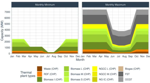
We defined must-run conditions for different seasons of the year, as many plants serve heat demand from the residential and industrial sectors. Generation in CHP plants was assumed to follow a monthly pattern throughout each year, with higher minimum production during the winter months, and lower minimum production during the summer. Additionally, maximum production was restricted during the summer period to account for maintenance and limited operation of CHP plants due to low heat demand. Annual production profiles were developed based on statistics of installed capacity and annual production per fuel type, in district heating systems and industrial back-pressure systems, respectively [47]. Expected annual full-load hour equivalents amount to 7500 h𝑎−1for industrial biomass CHP and waste CHP, and 5000 h 𝑎−1_{for biomass CHP plants [51].Fig. 1shows the load profiles applied}

in the optimisation model.

Maximum combined hourly ramping rates for the sum of ther-mal power generation were derived from historical observations of maximum ramping rates, and therefore set to 1.5 GW.

2.1.5. Hydrogen production

We have assumed that electrolyser technology will advance beyond the current commercial benchmark of alkaline electrolysis, to proton exchange membranes (PEM). Compared to alkaline electrolysis, PEM features higher efficiency, shorter start-up times, especially from cold, and a more extensive range for production rate variations [52]. Based on this, we set the hydrogen production efficiency to 72% (system efficiency, defined as hydrogen output on LHV basis divided by elec-trical input to the electrolysis system), which corresponds to 46 kWh of electricity per kg hydrogen [53,54]. The electrolyser was sized according to an expected electrolyser utilisation of 90%. As described in Section2.2.1, the utilisation of the electrolyser is a model output, which means that hydrogen demand in the different scenarios will not always be strictly met.

As PEM electrolysers in general are highly flexible, with start-up times and ramping in the range of minutes or even seconds and very low minimum part-load operation (<10%), neither ramping nor electrolyser part-load restrictions were considered in the model [52]. 2.2. Scenarios

We defined increasing levels of demand for hydrogen (four scenar-ios) and tested these demand scenarios under gradually more restricted flexibility in the system. First, we restricted thermal generation for hydrogen production by either allowing or not allowing the dispatch of thermal power generation for hydrogen production (two scenar-ios). Subsequently, we restricted the hydropower flexibility by limiting ramping and minimum river flows in two scenarios. This results in a total of 12 scenarios with hydrogen production plus two baseline scenarios without hydrogen demand (and therefore no thermal dispatch for hydrogen scenario).

Additionally, we ran a sensitivity analysis on the model for a wider set of hydrogen demands (see Section2.2.1).

Table 1

Costs and capacities used. (CHP=combined heat and power, RDF=refuse derived fuel, NG=natural gas, NGCC=natural gas combined cycle, FST=condensing steam turbine, OCGT=open cycle gas turbine, IC=internal combustion engine, S= small, M=medium, L=large, I=industrial.)

Production type Fuel type Installed capacity (MW) Costs (eMWh−1₎

Thermal plants Waste (CHP) Waste 315 −63.2 RDF (CHP) Waste 385 5.55 Biomass I (CHP) Biomass 1255 18.8 Biomass L (CHP)a _{Biomass 1318 21.0} Biomass M (CHP) Biomass 603 24.8 Biomass S (CHP) Biomass 401 30.9 NGCC L (CHP) NG 701 57.9 NGCC M (CHP) NG 54 74.1 NG IC (CHP) NG 13 83.4 FST Oil & NG 905 125 OCGT Oil 1579 152 Biogas IC (CHP) Biogas 21 156 Hydropower – 16,155b ₁ Wind – varyingc ₀

Additional backup measures – – 1500

Electrolysis – varyingc _varying

a_{This category also contains CHP plants currently using coal or peat as fuel (total installed capacity of 298 MW), as those} were assumed to have been replaced by biomass CHP.

b_{Installed capacity was corrected to13.6 GWin the simulations to reflect the maximum observed capacity in the29 yearsof} data available. This capacity is confirmed by Kan et al. [43] who take into account reduced capacities due to environmental regulation.

c_{Wind and electrolysis capacity are directly coupled, as explained in detail in Section2.2.1.}

Fig. 1. Modelled minimum (left) and maximum (right) thermal power production, per category. CHP=combined heat and power, RDF=refuse derived fuel, NG=natural gas, NGCC=natural gas combined cycle, FST=condensing steam turbine, OCGT=open cycle gas turbine, IC=internal combustion engine, S=small, M=medium, L=large, I= industrial.

2.2.1. Hydrogen demand

The hydrogen production scenarios were chosen so that they can deliver different amounts of hydrogen in order to satisfy different levels of future projected demand. We limited the hydrogen usage options to two pathways that are currently under development in Sweden: for hydrotreatment of different bio-based feedstocks in biofuel production, and as use as a reductant in fossil-free primary steelmaking accord-ing to the HYBRIT (Hydrogen Breakthrough Ironmakaccord-ing Technology) route. We applied four different hydrogen scenarios, where one is the baseline scenario without electrolysis-based hydrogen (No), and the

other three (Small, Medium, Large) can be considered as representing

either different ambition levels for decarbonisation or different time perspectives. This results in different electrolysis loads on the system, as outlined inTable 2.

Table 2

Modelled hydrogen demand scenarios. Scenario Hydrogen for

biofuels (TWh𝑎−1₎ Hydrogen for steelmaking (TWh𝑎−1₎ Electrolyser capacity (MW) No 0 0 0 Small 5 0 880 Medium 10 0 1760 Large 10 10 3610

The estimates regarding biofuel production build on the ambitions announced byPreem, Sweden’s largest fuel producer, who has a goal of producing 3 million m3_{of biofuels by 2030 in their two refineries in} Sweden [55]. Judging from Preem’s announced projects and plans, all

biofuels will be drop-in fuels produced via hydroprocessing of various bio-crudes. Hydrogen is currently produced from refinery off-gases or via steam reforming of natural gas, butPreemhas also expressed strong interest in hydrogen produced via electrolysis [55]. We based our scenarios on the assumption that electrolysis-based hydrogen will be the main pathway in the future, and implemented two different annual demand levels; 5 and 10 TWh hydrogen, respectively. The lower level represents a scenario in which a large share of the biofuel feedstock has a relatively low oxygen content (e.g., used cooking oils or bio-crudes produced via hydropyrolysis or hydrothermal liquefaction). In contrast, the higher scenario assumes a large share of biofuel feedstock with a higher oxygen content (e.g., lignin oil or fast pyrolysis oil) [56].

In the Large scenario, we also assumed that the HYBRIT route

will be fully implemented in Sweden and that all primary steelmaking via the blast furnace-basic oxygen furnace route will thus be replaced with hydrogen-based direct reduction followed by electric arc furnaces. We only considered the projected additional electricity demand to cover the required hydrogen production (10 TWh𝑎−1) [57], while we excluded the additional electricity demand from downstream processes, similar to other industrial electrification (see Section2.1.1).

The scenarios were implemented by changing the restriction on electrolyser capacity and scaling wind power in a way that on an annual average, wind power generates enough electricity to supply the electrolyser at full load. For instance, in an 880 MW electrolyser scenario, we added wind capacity that, on average, generates 880× 8760 MWh 𝑎−1_{. Thus, we could assess in how far the wind resource}

can be used for electrolysis and how much wind power is curtailed. Electrolyser utilisation was thus an output of the model, which means that the total defined hydrogen demand may not be exactly met in all scenarios if it is too costly to do so.

In addition to the scenarios based on announced plans by different industrial actors, we applied a sensitivity analysis, where we tested extended capacities of electrolysers – and associated increases in wind power generation – on a wide range of scenarios (5 GW to 50 GW). 2.2.2. Thermal power flexibility

In addition to varying the hydrogen demand, we also assessed the impact of dispatching thermal power plants for hydrogen production. Technically, we did so by varying the value of hydrogen in the objective function so that it was either below most (18eMWh−1_{) or above all}

(160 _eMWh−1_{) marginal costs of thermal generation. Thus, thermal}

power was either never or always dispatched to produce hydrogen. This represents two extreme settings, for which reason the results cover a wide range of possible outcomes. We refer to these scenarios asNo

thermalandThermal, respectively.

2.2.3. Hydropower flexibility

We assessed two different scenarios regarding the impact of seasonal ramping restrictions and seasonal flow thresholds in the hydropower system. The scenarios thus represent two different hydropower regula-tion development pathways.

The first scenario allowed for high flexibility in the hydropower operation, including the possibility for rapid flow fluctuations (Hi

hydro flex). The second scenario represented a more cautious

sce-nario designed to prevent adverse impacts on river ecosystems from hydropeaking and water retention throughout low flow seasons (Lo

hydro flex). We implemented the restrictions by limiting the

max-imum ramping rate (MRR) and minmax-imum flow (MF), following the approach proposed by Olivares et al. [58]. The limits were derived from the simulation of potential natural flows (i.e., without human intervention) from the S-HYPE model [46]. TheLo hydro flexscenario

was characterised by a very restrictive minimum flow rate of 50% and a maximum ramping rate of only 6% of the median natural flow. In

theHi hydro flexscenario, the minimum flow was restricted to 20%

and maximum ramping to 28% of the median natural flow. We observe the highest monthly median flow in June at about 18,000 MW, and

the lowest flow in March, at only 3600 MW, which leads to a high variation throughout the year of both minimum flows and maximum ramping rates. The resulting monthly limits are displayed inFig. 2, whereashows the minimum flow, andbthe maximum ramping rates. Fig. 2aalso shows the daily mean flows for all the 29 modelled weather years, assuming no human intervention (blue) and the actual historical daily mean flow of 16 modelled weather years, considering human interference.

2.3. Model runs and performance indicators

We ran the optimisation model for all scenarios outlined in the previous sections. Each scenario was evaluated for 29 different weather years, at hourly temporal resolution. Our evaluation focused on the following performance indicators:

• Utilisation of electrolysers (% of 8760 h)

• Inter-annual variability of hydrogen production (variance in util-isation across years)

• Thermal power generation (MWh𝑎−1₎

• Required additional backup capacity (MW) • Required additional backup energy (MWh𝑎−1)

• Variability in hydro flow (maximum hourly ramping) (MW) • Minimum hydro flow (MW)

3. Results and discussion

The results focus on the utilisation of electrolysers, thermal gen-eration, backup generation and capacity, and the changes in flows and minimum flows as induced by hydropower operation. We show the results of the base scenario without electrolyser operation where applicable.

3.1. Electrolyser utilisation

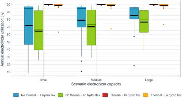
We first discuss here the electrolyser utilisation in the different scenarios.Fig. 3shows the annual utilisation rate in all 29 simulated years for all scenarios. The average utilisation rate is significantly lower for those scenarios that do not allow for the dispatch of thermal generation for hydrogen production. Additionally, lower hydropower flexibility decreases the utilisation rate — with some exceptions for single years, as discussed below. For theNo thermalscenarios with high

hydropower flexibility, the average utilisation rate is mainly lowered by some extreme years, as can be observed from the difference between the median and the mean of the distribution.

The average utilisation rate of the electrolyser increases with higher electrolyser and wind power capacities in theNo thermal scenarios,

while it decreases slightly for theThermalscenarios. The reason is that

in theNo thermalscenarios, the initial system response is that wind

power substitutes thermal power generation compared to the baseline scenario, as this reduces operational cost. However, this substitution effect is restricted by the required minimum generation of thermal power production caused by the residential and industrial heat demand. At higher electrolyser and wind capacities, this causes an increase of excess wind power to use in hydrogen production. Section3.5explores this effect in more detail.

The inter-annual variability of hydrogen production is very high for

theNo thermalscenarios, and the electrolyser utilisation even drops

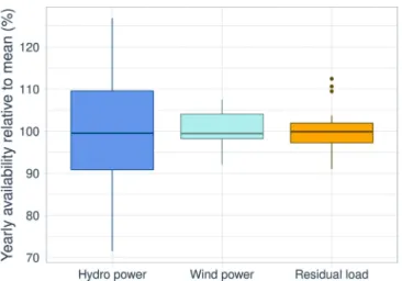
to below 25% for single years. This inter-annual variability is mainly driven by the variability in the availability of hydropower, and less so by the variability in wind power generation or temperature-dependent demand (seeFig. 4). In some cases, the utilisation rate in the scenario with higher hydropower flexibility is lower than in the corresponding scenarios with lower hydropower flexibility. The counter-intuitive re-sponse of the utilisation rate to hydropower flexibility requirements

Fig. 2. a: Minimum flow restriction (expressed as MW), andb: Maximum allowed ramping per hour (expressed as MW), for the two modelled flexibility scenarios.aalso shows the daily mean natural flow of 29 weather years and 16 years of regulated flow.

Fig. 3.Boxplots of annual electrolyser utilisation in all scenarios. The black lines show the mean over all years.

arises from the need to satisfy higher minimum flow requirements dur-ing the summer by drawdur-ing water from hydro reservoirs in theLo hydro flex scenario. During summertime, sufficient renewable electricity

from combined hydro and wind power generation is therefore available to operate electrolysers. As a consequence, reservoir filling levels are low during winter in years with low precipitation, and thermal power generation and backup generation events increase. Therefore, in low precipitation years, electrolyser utilisation can be higher inLo hydro flexthan inHi hydro flexscenarios.

The overall results in this section imply that single bad hydropower years have to be accounted for in the long-term planning of hydrogen supply if the dispatch of thermal capacities for hydrogen production should be prevented. Either long-term storage of hydrogen or alter-native supply routes have to be maintained in order to be equipped against low precipitation years.

3.2. Thermal generation

Fig. 5 shows the dispatch of thermal capacities in all scenarios. As could be expected, thermal generation is lower in theNo thermal

scenarios, with the obvious exception of the No hydrogen capacity

scenario. Thermal generation is, correspondingly, higher for the Lo

hydro flex scenarios. Limiting hydropower flexibility increases the

annual thermal power generation, on average, by 3 TWh in the No

scenario. In scenarios where thermal generation is not dispatched for electrolyser operation, the total thermal generation falls with increasing electrolyzer sizes because additional wind power capacity is added to the system. At some points in time, this wind power is not used to produce hydrogen but to substitute thermal generation. This is, conversely, not the case for theThermal scenarios, where the added

wind power generation does not replace thermal generation.

In theLargescenario, the difference in annual thermal generation

increases to on average 8 TWh when comparing the two most extreme scenarios, i.e., theNo thermal - Hi hydro flexand the Thermal -Lo hydro flexscenarios. In single years, this difference can go up to

20 TWh. Again, this shows that while thermal power production is not essential to achieve sufficient electrolyser utilisation on average, in single years the dispatch of thermal power for electrolyser operation will allow for significantly higher full load hours.

The share of thermal generation in total generation over the whole period is between 11% and 17%, depending on the scenario. A large share of this generation is due to must-run conditions of thermal power

Fig. 4. Annual variability of natural availability of hydropower, wind power, and temperature-dependent residual load.

plants, which have to generate at least 15 TWh𝑎−1_{of power to provide}

sufficient heat to heat consumers. Of course, in future systems with potentially lower heat consumption and alternative low-carbon heat sources, thermal generation may be reduced further. Appendix A.3 shows thermal dispatch in more detail.

3.3. Backup generation and capacity

Backup generation (Fig. 6) and capacity (Fig. 7) are both minor in all scenarios. If one extreme weather year, i.e. 1996, is removed from the data set, annual backup energy utilisation is lower than 82 GW h in all remaining years, with a required annual backup capacity lower than 4 GW in all scenarios. The backup generation and capacity both fall with increasing electrolyser capacity and corresponding wind power generation in the system, as electrolysers are ramped down in hours when backup operation would otherwise be necessary. Electrolysers, in tandem with the additional wind power generation capacities required for operation, can therefore provide essential value to the system

by reducing the amount of backup capacity necessary. In the Large

scenario, backup capacity requirements consequently fall to below 2.5 GW. The difference between the hydropower flexibility scenarios is minimal. Lower hydropower flexibility increases backup capacity and energy requirements, but mostly due to one extreme year.

All scenarios run on at least 83% of wind and hydropower, and only existing thermal generation capacities, excluding nuclear, are consid-ered. The resulting backup requirements are low, and in particular the energy provided by those backup capacities is negligible, even if high variable costs are assumed. Providing, in total, on average 0.08 TWh of annual backup in the form of, e.g., demand response in a system that has a total demand of at least 130 TWh seems to be on a realistic scale. 3.4. Hydropower ramping and minimum flows

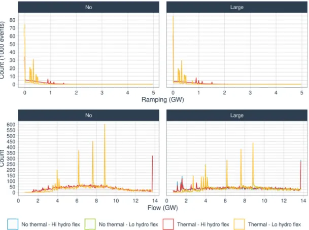
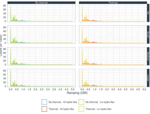
Fig. 8shows the distribution of hourly river flows and ramps in the system for the Noand Largescenarios. Appendix A.4shows all

scenarios in detail. The figure confirms that the flexibility restrictions work as expected: ramps are lower and minimum flows are higher when hydropower flexibility is restricted. In particular, the spread of the distribution of flows is narrower when the restrictions are tightened. Likewise, ramping is lower on average, in particular concerning the ramping maxima.

Higher electrolyser capacities slightly increase the spread in both river flows and magnitude of ramping events. Hydropower is therefore operated slightly more flexibly with increasing hydrogen production and added wind power capacity, as hydropower partly balances the in-creased system variability. There is almost no difference between theNo thermalandThermalscenarios if the same hydropower flexibility rules

are applied, i.e., using thermal generation for hydrogen production does not affect the extreme conditions of hydropower operation.

Interestingly, extreme ramping events are, although allowed, rare. The maximum ramping allowed in the scenario with low flexibility is just above 1 GW. However, this ramping capacity is required at most in 0.3% of all hours in all scenarios, while ramping above 0.75 GW is only necessary in at most 1.9% of all hours. Likewise, a ramping capacity above 2 GW is only required in at most 0.4% of all hours in the scenario with high hydropower flexibility, where around 5 GW of ramping is allowed. These results indicate that rapid ramping of hydropower is

Fig. 6.Annual backup energy (GWh𝑎−1_{) in all scenarios, the right panel without displaying extreme outliers (1996). Black lines show the mean over all years.}

Fig. 7.Annual required backup capacity (GW) in all scenarios. Black lines show the mean over all years.

beneficial to the system in some moments, but is not massively required to balance the system.

The peaks in the density plot of flows show the seasonal minima that have to be respected — they are in particular binding when the flexibility of hydropower generation is low. When the restriction on hydropower operation is relaxed, the flow distribution is much more diversified, i.e., there are significantly more of both very low and very high flow events, indicating that hydropeaking indeed may be a problem in systems with high shares of wind power generation. With the operation of electrolysers and the addition of wind turbines to the systems, the number of very large flows decreases. Instead, the number of very low flows increases, in particular for theHi hydro flex

scenarios.

3.5. Sensitivity analysis

Fig. 9shows the resulting utilisation of electrolysers when extend-ing the capacities to very high levels, also includextend-ing a correspondextend-ing expansion of wind power capacity.

The figure shows that an increase of the electrolyser capacity up to around 8 GW of capacity has a perhaps counter-intuitive consequence for theNo thermalscenarios: at the lower end of electrolyser capacities,

increasing capacities increase the electrolyser utilisation for the No

thermal scenarios, up to somewhere in the range of 5 GW to 10

GW of capacity, depending on the scenario. Above that point, adding more electrolyser (and wind) capacity reduces electrolyser utilisation. The cause is that at lower wind capacities, wind is used to cover residual demand in hours with abundant wind, as it is assumed to have zero marginal cost. Less wind is thus available for surplus hydrogen production due to that substitution. Increasing the wind power capacity in the system further will reduce the thermal generation to the defined minimum load, thus making no more substitution of thermal gener-ation possible and, instead, releasing a higher share of wind power generation for hydrogen production.

Therefore, rapidly increasing utilisation of electrolysers can be ob-served at the lower capacity range in the No thermal scenarios. At

Fig. 8.Density plots of hourly hydropower ramping (top) and flows (bottom) in theNoandLargehydrogen scenarios, over all hours.

Fig. 9. Average electrolyser full-load operation (%) for an extended electrolyser capacity range, for all scenarios. The three hydrogen demand scenarios are marked with vertical dotted lines; the curved lines show the adjusted electrolyser capacity to meet the expected yearly production (estimated at 90% for each scenario).

capacity for some hours. Once the latter effect overtakes the former, the utilisation starts decreasing again. This effect, however, applies only if no extra thermal power is dispatched for hydrogen production. In

theThermalscenario, where thermal power is dispatched for hydrogen

production, the utilisation starts falling with increasing electrolyser capacity immediately.

3.6. Limitations of the analysis

We have assessed multi-annual variability of hydrogen production in almost fully renewable electricity systems, considering flexibility from thermal and hydropower generation. This has, to the best of our knowledge, not been done before. In this section, we discuss limitations of our analysis.

We did not model the interaction between electricity and hydrogen markets. In bad weather years, electricity prices will increase, which will also drive up hydrogen prices. Depending on the relative effect on the two, either the markets will favour thermal dispatch for hydrogen production, thus limiting the negative impact of single bad weather years on hydrogen production, or hydrogen production will decrease.

We also assumed that Sweden has no international interconnections and that internally, there are no transmission bottlenecks. The first assumption makes our results conservative, as the existing interconnec-tions clearly could provide backup capacities. At the same time, market prices and dispatch would change significantly, if interconnections would be taken into consideration. Depending on the thermal flexibility scenario, thermal power generation in neighbouring countries would be replaced by Swedish wind power generation up to the interconnector capacity, before generating surplus electricity for hydrogen production within the country. Disregard of international interconnections also implies that Sweden has net zero exports and imports, which can be compared to current annual exports of around 10 TWh to 20 TWh of electricity. The second assumption, which neglects internal restrictions in transmission, is an obvious simplification. Here, we assume that the transmission grid is reinforced to accommodate additional wind power and prevent frequent large-scale curtailment.

Land and sea availability for placing wind-turbines is another major issue. In the scenario with the largest electrolyser capacity (3610 MW), around 100 TWh𝑎−1_{of wind power is generated, requiring the}

installa-tion of around 30 GW of wind power capacity. In comparison, Germany had an installed capacity of above 50 GW of wind in 2019, while only having 80% of the available land area of Sweden. Such an expansion should thus in principle be possible. It may, however, cause regional environmental impacts and land conflicts, and mitigation measures must be taken seriously.

Further, we modelled hydropower operation on an aggregated level for the whole of Sweden. Therefore, detailed assessments of environ-mental impacts are not possible. Also, some of the dispatch schedules may be physically impossible once down-scaled to the level of river basins. We recommend more work here.

Direct reduction is one among several pathways that have been sug-gested for lowering the carbon intensity in steelmaking. Other options include top gas recycling for the blast furnace, increased electrifica-tion and carbon capture and storage (CCS) (e.g., [59,60]), as well as the introduction of bioenergy and bio-reducers in combination with CCS [61], and iron ore electrolysis via so-called electrowinning [62]. Only three pathways offer the possibility to reduce the CO2emissions to near zero; direct reduction based on renewable hydrogen, CCS of all furnace gases, and the more theoretical concept of electrowinning [57]. We chose to focus on hydrogen for steelmaking as this pathway has gained substantial attention during recent years. Besides the HYBRIT initiative in Sweden, several other European steelmakers have initi-ated major projects in this direction, e.g., Salzgitter (Germany) and Voestalpine (Austria) [63].

We only considered increased load from the electrolysis, which makes our electricity demand scenarios rather conservative. Other sce-narios show a potential increase from the electrification of, e.g., trans-port and (other parts of) the industry where the total annual electricity demand may increase to over 200 TWh, including demand from elec-trolysis [64]. This compares to a load of about 130 TWh 𝑎−1in our scenario without electrolyser, and around 160 TWh 𝑎−1 in our most extensive electrolysis scenario. At the same moment, we assume that around 60 TWh𝑎−1of nuclear are phased out. Keeping nuclear in the system would therefore be able to cover additional demand from other sectors at least partly.

4. Conclusions

We have assessed how electrolyser operation evolves if a defined amount of hydrogen on an inter-annual average should be produced

and if power demand of electrolysers is met on average by new wind power capacities for our Swedish case study. We have shown that while in all scenarios the average annual utilisation of electrolysers is above 60%, the inter-annual variability of hydrogen production is high unless thermal power is dispatched for electrolysis.

Furthermore, if hydropower flexibility is additionally restricted to reduce hydropeaking and running dry of rivers, the inter-annual vari-ability is increased further. As the maximum constraints in hydropower generation are, however, only met rarely, one important policy con-clusion is that allowing for high, yet rare, extreme operation of hy-dropower, can make the whole system more resilient. This calls for more research on the ecological impacts of rare hydropeaking events and a detailed, river-scale assessment of hydropower generation under extensive penetration of variable renewables.

Due to high inter-annual variability, either long-term storage of hydrogen, backup hydrogen sources or dispatch of thermal capacities in extreme years is, therefore, necessary to maintain a stable hydrogen flow to the industry. This means that on average hydrogen costs can be low, but extreme years with high costs have to be expected. We did not explicitly assess the costs of hydrogen production; however, our results, openly available, can provide fundamental input to such kind of analysis by others.

Adding more wind power to the system while also adding large electrolyser capacity as a primary consumer of the wind power makes the system more stable, if electrolysers ramp down in rare hours of extreme events with low availability of renewable generation. The need for additional backup capacities in a fully renewable Swedish electricity system is reduced in a system that combines wind power and large-scale electrolysis based hydrogen production.

CRediT authorship contribution statement

Christian Mikovits: Conceptualization, Methodology, Software, Validation, Data curation, Formal analysis, Investigation, Writing -original draft, Writing - review & editing, Visualization. Elisabeth Wetterlund:Conceptualization, Data curation, Investigation, Writing -original draft, Writing - review & editing, Supervision, Project adminis-tration, Funding acquisition.Sebastian Wehrle:Software, Validation, Data curation, Writing - original draft, Writing - review & editing. Johann Baumgartner:Validation, Formal analysis, Writing - original draft.Johannes Schmidt:Conceptualization, Methodology, Software, Validation, Data curation, Formal analysis, Investigation, Writing -original draft, Writing - review & editing, Visualization, Supervision, Funding acquisition.

Declaration of competing interest

The authors declare that they have no known competing finan-cial interests or personal relationships that could have appeared to influence the work reported in this paper.

Acknowledgements

The Swedish Research Council Formas (dnr. 2016–20118) and Bio4Energy, Sweden financially supported this work. We also grate-fully acknowledge support from the European Research Council (‘‘re-FUEL’’ ERC2017-STG 758149) and by CLIM2POWER, Sweden. Project CLIM2POWER is part of ERA4CS, an ERA-NET initiated by JPI Climate and funded by FORMAS (SE), BMBF (DE), BMWFW (AT), FCT (PT), EPA (IE), ANR (FR) with co-funding by the European Union (Grant 690462). We would also like to thank SMHI, the Swedish Meteorological and Hydrological Institute, for providing the S-Hype data.

Table A.3

Sets used.

Name Symbol Unit Elements

Time steps ℎ h ℎ1, ℎ2,…, ℎ𝑛

Technologies 𝑡𝑦𝑝𝑒 – SeeTable A.6

Appendix. Model description

We employ a deterministic model to optimise the dispatch of hy-dropower and thermal power production. The model determines system costs minimising the hourly dispatch costs of thermal power plants while meeting the hourly demand.

A.1. Mathematical description A.1.1. Sets

All parameters and variables are defined over the sets given in Table A.3.

A.1.2. Parameters

Table A.4 summarises the used hourly data, parameters and vari-ables.

A.1.3. Variables

Modelled variables are Summarised inTable A.5. A.1.4. Objective

The objective function is given by Eq. (A.1), which represents dispatch costs𝑑𝑖𝑠𝑝𝑎𝑡𝑐ℎ_𝑐𝑜𝑠𝑡in the system over one year.

min𝑑𝑖𝑠𝑝𝑎𝑡𝑐ℎ_𝑐𝑜𝑠𝑡=∑ ℎ ( ∑ 𝑡𝑦𝑝𝑒 𝑥_𝑡ℎ𝑒𝑟𝑚𝑎𝑙_{ℎ,𝑡𝑦𝑝𝑒}⋅𝑐_{𝑡𝑦𝑝𝑒}𝑡ℎ +𝑐ℎ𝑜⋅𝑥_ℎ𝑦𝑑𝑟𝑜_ℎ+ 0.5⋅𝑐ℎ𝑜⋅𝑥_𝑠𝑝𝑖𝑙𝑙_ℎ +𝑥_𝑏𝑎𝑐𝑘𝑢𝑝_𝑑𝑖𝑠𝑝𝑎𝑡𝑐ℎ_ℎ⋅𝑐𝑏𝑑−𝑥_ℎ2ℎ⋅𝑝ℎ2 ) (A.1)

The costs are given by the sum of dispatching thermal power production (𝑥_𝑡ℎ𝑒𝑟𝑚𝑎𝑙ℎ,𝑡𝑦𝑝𝑒) with cost 𝑐𝑡𝑦𝑝𝑒𝑡ℎ , and dispatching backup generation 𝑥_𝑏𝑎𝑐𝑘𝑢𝑝_𝑑𝑖𝑠𝑝𝑎𝑡𝑐ℎ_ℎ with cost 𝑐𝑏𝑑_{. We also assign costs to} hydropower production𝑥_ℎ𝑦𝑑𝑟𝑜_ℎand to spilling of water𝑥_𝑠𝑝𝑖𝑙𝑙_ℎ. These costs are set very low and represent variable costs in the hydropower plant. The future value of water is not considered in our deterministic approach. As the produced hydrogen𝑥_ℎ2ℎhas a market value𝑝ℎ2, it enters negatively into the objective function.

A.1.5. Constraints

The residual demand 𝑑𝑒𝑚𝑎𝑛𝑑_ℎ, potential curtailments 𝑥_𝑐𝑢𝑟𝑡𝑎𝑖𝑙𝑚𝑒𝑛𝑡_ℎ, and hydrogen production has to be met in all time instances by generation of hydropower and thermal power, as shown in Eq.(A.2). 𝑑𝑒𝑚𝑎𝑛𝑑_ℎ=𝑥_ℎ𝑦𝑑𝑟𝑜_ℎ+∑ 𝑡𝑦𝑝𝑒 (𝑥_𝑡ℎ𝑒𝑟𝑚𝑎𝑙_{ℎ,𝑡𝑦𝑝𝑒}) +𝑥_𝑏𝑎𝑐𝑘𝑢𝑝_𝑑𝑖𝑠𝑝𝑎𝑡𝑐ℎ_ℎ −𝑥_𝑐𝑢𝑟𝑡𝑎𝑖𝑙𝑚𝑒𝑛𝑡_ℎ−𝑥_ℎ2ℎ ∀ℎ (A.2) Installed capacities of thermal power plants 𝑡ℎ𝑒𝑟𝑚𝑎𝑙_𝑐𝑎𝑝_{𝑡𝑦𝑝𝑒} and electrolysersℎ2_𝑐𝑎𝑝are defined in Eqs.(A.3)and(A.4).

𝑥_𝑡ℎ𝑒𝑟𝑚𝑎𝑙_{ℎ,𝑡𝑦𝑝𝑒}≤𝑡ℎ𝑒𝑟𝑚𝑎𝑙_𝑐𝑎𝑝_{𝑡𝑦𝑝𝑒} ∀ℎ, 𝑡𝑦𝑝𝑒 (A.3)

𝑥_ℎ2_ℎ≤ℎ2_𝑐𝑎𝑝 ∀ℎ (A.4)

Restrictions on thermal generation 𝑥_𝑡ℎ𝑒𝑟𝑚𝑎𝑙_{ℎ,𝑡𝑦𝑝𝑒} are defined by the following equations. Minimum 𝑚𝑖𝑛_𝑡ℎ𝑒𝑟𝑚𝑎𝑙_{ℎ,𝑡𝑦𝑝𝑒} and maximum 𝑚𝑎𝑥_𝑡ℎ𝑒𝑟𝑚𝑎𝑙_{ℎ,𝑡𝑦𝑝𝑒} thermal generation by type are controlled by Eqs.(A.5)and(A.6).

𝑥_𝑡ℎ𝑒𝑟𝑚𝑎𝑙_{ℎ,𝑡𝑦𝑝𝑒}⩾𝑚𝑖𝑛_𝑡ℎ𝑒𝑟𝑚𝑎𝑙_{ℎ,𝑡𝑦𝑝𝑒} ∀ℎ, 𝑡𝑦𝑝𝑒 (A.5)

𝑥_𝑡ℎ𝑒𝑟𝑚𝑎𝑙_{ℎ,𝑡𝑦𝑝𝑒}⩽𝑚𝑎𝑥_𝑡ℎ𝑒𝑟𝑚𝑎𝑙_{ℎ,𝑡𝑦𝑝𝑒}, ∀ℎ, 𝑡𝑦𝑝𝑒 (A.6) Thermal ramping, summed over all types, is constrained by Eqs.(A.7)and(A.8).

∑ 𝑡𝑦𝑝𝑒 (𝑥_𝑡ℎ𝑒𝑟𝑚𝑎𝑙_{ℎ,𝑡𝑦𝑝𝑒}) −∑ 𝑡𝑦𝑝𝑒 (𝑥_𝑡ℎ𝑒𝑟𝑚𝑎𝑙_{ℎ−1,𝑡𝑦𝑝𝑒}) ⩽𝑚𝑎𝑥_𝑡ℎ𝑒𝑟𝑚𝑎𝑙_𝑟𝑎𝑚𝑝 ∀ℎ (A.7) ∑ 𝑡𝑦𝑝𝑒 (𝑥_𝑡ℎ𝑒𝑟𝑚𝑎𝑙_ℎ−1,𝑡𝑦𝑝𝑒) − ∑ 𝑡𝑦𝑝𝑒 (𝑥_𝑡ℎ𝑒𝑟𝑚𝑎𝑙_{ℎ,𝑡𝑦𝑝𝑒}) ⩽𝑚𝑎𝑥_𝑡ℎ𝑒𝑟𝑚𝑎𝑙_𝑟𝑎𝑚𝑝 ∀ℎ (A.8)

Additional constraints on hydro flow, ramping, and storage level are controlled with the following equations:

The reservoir level is limited on the upside by reservoir capacity. 𝑥_𝑟𝑒𝑠𝑒𝑟𝑣𝑜𝑖𝑟_𝑙𝑒𝑣𝑒𝑙ℎ ≤𝑟𝑒𝑠_𝑐𝑎𝑝 ∀ℎ (A.9) At the beginning of the year, reservoirs are partly filled.

𝑥_𝑟𝑒𝑠𝑒𝑟𝑣𝑜𝑖𝑟_𝑙𝑒𝑣𝑒𝑙_ℎ=𝑠𝑡𝑎𝑟𝑡_𝑟𝑒𝑠_𝑓 𝑖𝑙𝑙 for ℎ∈ {ℎ₁} (A.10) The reservoir level𝑥_𝑟𝑒𝑠𝑒𝑟𝑣𝑜𝑖𝑟_𝑙𝑒𝑣𝑒𝑙_ℎat the end of each simulated year is controlled by Eq. (A.11), which ensures that the level is above 𝑚𝑖𝑛_𝑟𝑒𝑠_𝑓 𝑖𝑙𝑙_𝑒𝑛𝑑.

𝑥_𝑟𝑒𝑠𝑒𝑟𝑣𝑜𝑖𝑟_𝑙𝑒𝑣𝑒𝑙_ℎ⩾𝑚𝑖𝑛_𝑟𝑒𝑠_𝑓 𝑖𝑙𝑙_𝑒𝑛𝑑 for ℎ∈ {ℎ_𝑛} (A.11) At no point in time can the reservoir level fall below minimum filling.

𝑥_𝑟𝑒𝑠𝑒𝑟𝑣𝑜𝑖𝑟_𝑙𝑒𝑣𝑒𝑙_ℎ≥𝑚𝑖𝑛_𝑟𝑒𝑠_𝑓 𝑖𝑙𝑙 ∀ℎ (A.12) Eq.(A.13)ensures that the reservoir level𝑥_𝑟𝑒𝑠𝑒𝑟𝑣𝑜𝑖𝑟_𝑙𝑒𝑣𝑒𝑙_ℎof one specific hour equals the reservoir level of the previous hour, plus the natural inflow 𝑛𝑎𝑡𝑢𝑟𝑎𝑙_𝑖𝑛𝑓 𝑙𝑜𝑤_ℎ, minus the outflow (hydropower production𝑥_ℎ𝑦𝑑𝑟𝑜_ℎand spill𝑥_𝑠𝑝𝑖𝑙𝑙_ℎ).

𝑥_𝑟𝑒𝑠𝑒𝑟𝑣𝑜𝑖𝑟_𝑙𝑒𝑣𝑒𝑙_ℎ=𝑥_𝑟𝑒𝑠𝑒𝑟𝑣𝑜𝑖𝑟_𝑙𝑒𝑣𝑒𝑙_ℎ−1+𝑛𝑎𝑡𝑢𝑟𝑎𝑙_𝑖𝑛𝑓 𝑙𝑜𝑤_ℎ

−𝑥_ℎ𝑦𝑑𝑟𝑜_ℎ−𝑥_𝑠𝑝𝑖𝑙𝑙_ℎ ∀ℎ (A.13) The minimum flow in each hour is controlled by Eq.(A.14), which ensures that hydropower production 𝑥_ℎ𝑦𝑑𝑟𝑜_ℎ and hydro spilling 𝑥_𝑠𝑝𝑖𝑙𝑙_ℎis larger than the minimum flow𝑚𝑖𝑛_𝑓 𝑙𝑜𝑤_ℎ.

𝑥_ℎ𝑦𝑑𝑟𝑜_ℎ+𝑥_𝑠𝑝𝑖𝑙𝑙_ℎ⩾𝑚𝑖𝑛_𝑓 𝑙𝑜𝑤_ℎ ∀ℎ (A.14) Likewise, the maximum possible flow 𝑚𝑎𝑥_𝑓 𝑙𝑜𝑤_ℎ is defined by Eq.(A.15).

𝑥_ℎ𝑦𝑑𝑟𝑜_ℎ+𝑥_𝑠𝑝𝑖𝑙𝑙_ℎ⩽𝑚𝑎𝑥_𝑓 𝑙𝑜𝑤_ℎ ∀ℎ (A.15) The maximum change in total flow per hour (maximum ramping, MRR) 𝑚𝑎𝑥_ℎ𝑦𝑑𝑟𝑜_𝑟𝑎𝑚𝑝_ℎis defined by Eqs.(A.16)and(A.17).

𝑥_ℎ𝑦𝑑𝑟𝑜_ℎ+𝑥_𝑠𝑝𝑖𝑙𝑙_ℎ−𝑥_ℎ𝑦𝑑𝑟𝑜_ℎ−1−𝑥_𝑠𝑝𝑖𝑙𝑙_ℎ−1⩽𝑚𝑎𝑥_ℎ𝑦𝑑𝑟𝑜_𝑟𝑎𝑚𝑝_ℎ ∀ℎ (A.16) 𝑥_ℎ𝑦𝑑𝑟𝑜_ℎ−1+𝑥_𝑠𝑝𝑖𝑙𝑙_ℎ−1−𝑥_ℎ𝑦𝑑𝑟𝑜_ℎ−𝑥_𝑠𝑝𝑖𝑙𝑙_ℎ⩽𝑚𝑎𝑥_ℎ𝑦𝑑𝑟𝑜_𝑟𝑎𝑚𝑝_ℎ ∀ℎ

(A.17) Maximum ramping𝑚𝑎𝑥_ℎ𝑦𝑑𝑟𝑜_𝑝𝑟𝑜𝑑_𝑟𝑎𝑚𝑝of hydropower production 𝑥_ℎ𝑦𝑑𝑟𝑜_ℎis controlled by Eqs.(A.18)and(A.19).

𝑥_ℎ𝑦𝑑𝑟𝑜_ℎ−𝑥_ℎ𝑦𝑑𝑟𝑜_ℎ−1⩽𝑚𝑎𝑥_ℎ𝑦𝑑𝑟𝑜_𝑝𝑟𝑜𝑑_𝑟𝑎𝑚𝑝 ∀ℎ (A.18)

𝑥_ℎ𝑦𝑑𝑟𝑜_ℎ−1−𝑥_ℎ𝑦𝑑𝑟𝑜ℎ⩽𝑚𝑎𝑥_ℎ𝑦𝑑𝑟𝑜_𝑝𝑟𝑜𝑑_𝑟𝑎𝑚𝑝 ∀ℎ (A.19) The hourly wind production 𝑤𝑖𝑛𝑑_ℎ restricts wind curtailment 𝑥_𝑐𝑢𝑟𝑡𝑎𝑖𝑙𝑚𝑒𝑛𝑡_ℎ in Eq.(A.20); wind can thus be curtailed from 0% to 100%.

Fig. A.10. Resulting thermal power load duration curves, per production type (aggregated), on an hourly basis over all 29 years. Top:Nohydrogen scenario, middle:Largein combination withNo Thermal, bottom:Largehydrogen in combination withThermal. Left:Hi hydro flex, right:Lo hydro flex.

Fig. A.11. Load duration curves for additional backup capacity. Top:Nohydrogen, middle:Largehydrogen andNo thermal, bottom:Largehydrogen withThermal. Left:Hi hydro flex, rightLo hydro flex.

Table A.4

Parameters used.

Name Symbol Unit Value

Time series

Residual demand 𝑑𝑒𝑚𝑎𝑛𝑑ℎ MW See Section2.1.1

Natural inflow 𝑛𝑎𝑡𝑢𝑟𝑎𝑙_𝑖𝑛𝑓 𝑙𝑜𝑤ℎ MW See Section2.1.3

Wind production 𝑤𝑖𝑛𝑑ℎ MW See Section2.1.2

Cost & Prices

Costs of thermal generation by type 𝑐𝑡ℎ

𝑡𝑦𝑝𝑒 eMWh

−1 _{SeeTable A.6}

Cost of backup generation 𝑐𝑏𝑑 _eMWh−1 ₁₅₀₀

Cost of hydroelectricity generation 𝑐ℎ𝑜 _eMWh−1 _0.01 Market price of hydrogen produced 𝑝ℎ2 _eMWh−1 _{18 ∥ 160}

Capacities, Ramps & Restrictions

Thermal capacity by type 𝑡ℎ𝑒𝑟𝑚𝑎𝑙_𝑐𝑎𝑝_{𝑡𝑦𝑝𝑒} MW SeeTable 1

Electrolysis capacity ℎ2_𝑐𝑎𝑝 MW SeeTable 2

Storage fill at beginning of year 𝑠𝑡𝑎𝑟𝑡_𝑟𝑒𝑠_𝑓 𝑖𝑙𝑙 MW 62 %of reservoir capacity Minimum storage fill at end of year 𝑚𝑖𝑛_𝑟𝑒𝑠_𝑓 𝑖𝑙𝑙_𝑒𝑛𝑑 MW 62 %of reservoir capacity

Reservoir capacity 𝑟𝑒𝑠_𝑐𝑎𝑝 TW h 33.70

Minimum fill level of reservoir 𝑚𝑖𝑛_𝑟𝑒𝑠_𝑓 𝑖𝑙𝑙 MW h 5 %of reservoir capacity

Hydro generation capacity ℎ𝑦𝑑𝑟𝑜_𝑐𝑎𝑝 GW 13.73

Minimum hydro flow 𝑚𝑖𝑛_𝑓 𝑙𝑜𝑤_ℎ MW SeeFig. 2

Maximum hydro flow 𝑚𝑎𝑥_𝑓 𝑙𝑜𝑤_ℎ MW SeeFig. 2

Maximum hydro flow ramp 𝑚𝑎𝑥_ℎ𝑦𝑑𝑟𝑜_𝑟𝑎𝑚𝑝ℎ MW SeeFig. 2 Maximum hydro production ramp 𝑚𝑎𝑥_ℎ𝑦𝑑𝑟𝑜_𝑝𝑟𝑜𝑑_𝑟𝑎𝑚𝑝 GW 4.00 Minimum thermal production by type 𝑚𝑖𝑛_𝑡ℎ𝑒𝑟𝑚𝑎𝑙ℎ,𝑡𝑦𝑝𝑒 MW SeeFig. 1 Maximum thermal production by type 𝑚𝑎𝑥_𝑡ℎ𝑒𝑟𝑚𝑎𝑙ℎ,𝑡𝑦𝑝𝑒 MW SeeFig. 1 Maximum thermal ramping 𝑚𝑎𝑥_𝑡ℎ𝑒𝑟𝑚𝑎𝑙_𝑟𝑎𝑚𝑝 GW 1.50

Table A.5

Variables used.

Name Symbol Unit

Thermal electricity generation 𝑥_𝑡ℎ𝑒𝑟𝑚𝑎𝑙ℎ,𝑡𝑦𝑝𝑒 MW Electricity generation from backup 𝑥_𝑏𝑎𝑐𝑘𝑢𝑝_𝑑𝑖𝑠𝑝𝑎𝑡𝑐ℎℎ MW

Hydro electricity generation 𝑥_ℎ𝑦𝑑𝑟𝑜ℎ MW

Hydro spilling 𝑥_𝑠𝑝𝑖𝑙𝑙ℎ MW

Electricity input of electrolysers 𝑥_ℎ2ℎ MW Curtailed electricity generation 𝑥_𝑐𝑢𝑟𝑡𝑎𝑖𝑙𝑚𝑒𝑛𝑡_ℎ MW Reservoir filling level 𝑥_𝑟𝑒𝑠𝑒𝑟𝑣𝑜𝑖𝑟_𝑙𝑒𝑣𝑒𝑙_ℎ MW

A.2. Input data for thermal power production costs

Table A.6 summarises the key plant data used to calculate the thermal power production costs, and Table A.7 the fuel costs and fuel-related CO₂emission factors.

Power production costs were set based on bottom-up technology and fuel-specific projections of electricity generation costs [51,65], and were adjusted toe2018using the average 2018 currency exchange rate of 1e=10.3 SEK [66] and updated fuel prices. The production costs consists of fuel costs including a CO2-charge (50 e/tCO₂), costs for operation and maintenance (O&M), and heat credits, when applicable.

A.3. Detailed results on thermal power production and need for backup capacity

Fig. A.10shows load duration curves of the resulting dispatched thermal generation in two of the analysed hydrogen demand scenarios

(No andLarge), for both No thermalandThermal, and for the two

hydropower flexibility scenarios. The curves are derived from all 29 weather years (total of about 254,000 h).

The left column always shows lower thermal generation than the right column, indicating that decreasing hydropower flexibility will increase thermal dispatch. The first row shows a situation without electrolysers. Thermal power production is dominated by biomass gen-eration, with a small base-load production from waste incineration. Here, biomass plants and partly peaking plants from natural gas and oil are dispatched to balance wind power in the system.

The mid-row shows theNo thermalscenarios for aLarge

electrol-yser capacity. It is a situation where thermal generation is at its almost constrained minimum, as it is not dispatched for hydrogen production and wind power capacities in the system are high. Natural gas and oil plants are almost not dispatched.

In the bottom row, theThermalscenarios for theLargeelectrolyser

capacity scenarios are shown. The dispatch of biomass capacities is significantly increased here, as well as peaking natural gas and oil plants. This indicates that to achieve high utilisation of electrolysers

Table A.6

Technical data for the modelled thermal power plants [51,65]. CHP=combined heat and power, RDF=refuse-derived fuel, NG=natural gas, NGCC=natural gas combined cycle, FST=condensing steam turbine, OCGT=open cycle gas turbine, IC=internal combustion engine, S=small, M=medium, L=large, I=industrial. SeeTable 1for additional details.

Production type Power prod. (MW) Heat prod. (MW) El. efficiency (%) Alfa value Var. O&M (eMWh−1_{fuel) Fixed O&M (ekW}−1_𝑎−1_el.)

Waste (CHP) 20 78 20 0.256 5.26 215 RDF (CHP) 20 70 22 0.286 5.46 166 Biomass I (CHP) 80 180 33 0.444 2.63 37.0 Biomass L (CHP)a _{80 180 33 0.444 2.63 37.0} Biomass M (CHP) 30 72 32 0.417 2.53 56.5 Biomass S (CHP) 10 28 28 0.357 2.44 89.7 NGCC-L (CHP) 150 115 53 1.30 0.78 19.5 NGCC-M (CHP 40 35 49 1.14 0.97 29.2 NG-IC (CHP) 1 1.2 41 0.833 3.9 0 Oil/NG FST 300 0 38 – 4.66 14.3 Oil OCGT 300 0 34 – 5.21 10.1 Biogas IC (CHP) 1 1.2 41 0.833 3.9 0

Fig. A.12. Density plots of hourly hydro ramps over for all scenarios. Panels leftNo Thermaland rightThermal, from top to bottom: electrolyser capacity.