How Prepared Are State and Local Workers for Retirement

(1)

State and Local Pension Plans

Number 22, October 2011

HOW PREPARED ARE STATE AND LOCAL

WORKERS FOR RETIREMENT?

By Alicia H. Munnell, Jean-Pierre Aubry, Josh Hurwitz, and Laura Quinby*

* Alicia H. Munnell is the director of the Center for Retirement Research at Boston College (CRR) and the Peter F. Drucker Professor of Management Sciences at Boston College’s Carroll School of Management. Jean-Pierre Aubry is the assistant director of state and local research at the CRR. Josh Hurwitz and Laura Quinby are research associates at the CRR. This research was funded by a grant from Great-West Retirement Services. The authors would like to thank Beth Almeida, Frank Caine, and Nathan Scovronick for helpful comments.

Introduction

A widespread perception is that state-local govern-ment workers receive high pension benefits which, combined with Social Security, provide more than adequate retirement income. The perception is con-sistent with multiplying the 2-percent benefit factor in most plan formulae by a 35- to 40-year career and adding a Social Security benefit. But this calculation assumes that individuals spend enough of their career in the public sector to produce such a retirement out-come. This brief summarizes the results of a paper that uses the Health and Retirement Study (HRS) and actuarial reports published by state and local pension systems to test the hypothesis that state-local workers have more than enough money for retirement.1

The first section explores how much income peo-ple need in retirement and raises some conceptual

is-sues involved in constructing replacement rates. The second section presents replacement rates derived from Social Security and from employer-sponsored plans for individual workers in the private and state-local sectors. The third section replicates the analysis for households. The fourth section reports how non-pension financial assets affect the replacement rate picture. The fifth section summarizes the actuarial report evidence. The sixth section concludes.

The major finding from the HRS analysis is that most households with state-local employment end up with replacement rates that, while on average higher than those in the private sector, are well below the 80 percent needed to maintain pre-retirement living standards. Even those households with a long-service state-local worker – those who spend more than half of their careers in public employment – have a medi-an replacement rate, including Social Security, of only

LEARN MORE

Search for other publications on this topic at:

crr.bc.edu

(2)

72 percent. And this group accounts for less than 30 percent of households with a state-local worker. The remaining 70 percent of households with a short- or medium-tenure state-local worker have replacement rates of 48 percent and 57 percent, respectively. Add-ing income from financial assets still leaves most households short of the target.

Data from the actuarial reports provide part of the explanation for these lower-than-anticipated replace-ment rates. Only 32 percent of workers who leave state-local employment each year claim an immediate benefit. These individuals have more than 20 years of service on average and receive a benefit equal to 49 percent of their pre-retirement earnings. But another 27 percent leave state-local employment with a de-ferred benefit based on their earnings at termination, which will decline in value between termination and claiming as wages and prices rise, so it will amount to less than 10 percent of their projected earnings at retirement. And 40 percent leave without any prom-ise of future benefits. The other part of the explana-tion is that most households with a state-local worker contain a person employed in the private sector, and replacement rates for private sector workers are con-siderably lower since many end up with nothing more than Social Security.2

The “Replacement Rate” Concept

Replacement rates are used to gauge the extent to which older people can maintain their pre-retirement levels of consumption once they stop working.3_The most direct approach would be a comparison of household consumption while working with con-sumption after retirement. But such data are rarely available. An indirect approach is to compare pre- and post-retirement income.4_{This section briefly} reviews what might be considered an adequate level of replacement income and describes some of the conceptual issues involved in constructing replace-ment rates.

What Replacement Rate do People Need in Retirement?

People clearly need less than their full pre-retirement income to maintain their standard of living once they stop working. One big difference before and after retirement is the extent to which income is taxed. When people are working, their earnings are subject

to both Social Security and Medicare payroll taxes and federal personal income taxes. After retirement, they no longer pay payroll taxes, and they pay lower federal income taxes because only a portion of Social Security benefits are taxable. Under current law, individu-als with less than $25,000 and married couples with less than $32,000 of “combined income” do not have to pay taxes on their Social Security benefits. Above those thresholds, recipients must pay taxes on either 50 or 85 percent of their benefits.5

A second reason why retirees require less than their full pre-retirement income is that they no longer need to save a portion of that income for retirement. In addition to contributing to 401(k) plans, many households try to pay off their mortgage before they retire. In retirement, these households no longer need to save and, in fact, can draw on their accumu-lated reserves. Thus, a greater share of their income is available for consumption.

A final factor often mentioned is that work-related expenses, such as clothing and transportation, are either no longer necessary or are much reduced. Al-though this factor often tops many analysts’ lists, it is relatively small compared to taxes and saving.

While all analysts cite the same factors for why retirees need less than their full pre-retirement income, they employ different approaches to calculat-ing precisely how much less. The RETIRE Project at Georgia State University has been calculating re-quired replacement rates – that is, retirement income as a percent of pre-retirement earnings – for decades.6 As of 2008, the Project estimated that a couple with an income of $50,000 required 81 percent of pre-retirement earnings to maintain the same level of consumption (see Table 1). Couples earning $90,000 needed 78 percent, and couples earning $20,000 needed 94 percent, because they save very little before retirement and enjoy less in the way of tax reduction.

Table 1. Percent of Pre-Retirement Salary Required to Maintain Living Standards, 2008

Pre-retirement earnings

Two–earner

couples Single workers

$20,000 94 88

$50,000 81 80

$90,000 78 81

(3)

Constructing Replacement Rates

Constructing replacement rates raises a number of issues. The first question is the relevant measure of pre-retirement earnings. Social Security – the prima-ry source of monthly cash income for today’s elderly Americans – replaces a portion of “average indexed monthly earnings” (AIME), which is essentially the 35 highest years of earnings indexed to the present by wage growth.7_{Employer-sponsored defined benefit} plans – the other source of monthly income – typi-cally replace a portion of the worker’s annual earnings during the last three or five years of employment, which tend to be the worker’s highest earnings with that employer. Thus pre-retirement income could be defined as: 1) some measure of lifetime earnings; 2) earnings with a particular employer; or 3) earnings just prior to retirement. This study uses earnings just before retirement, defined as the highest five in the last ten years adjusted for inflation, because it pro-vides a measure of the end-of career standard of living that workers seek to maintain in retirement.

A second consideration is defining when “pre-retirement” ends and retirement begins. With the growth of bridge jobs, it is often impossible to define precisely the work/retirement divide. For this reason, this study focuses on the first year that workers start receiving Social Security benefits. In the case of couples, retirement is defined as when both members of the household are receiving benefits.

A third consideration is the unit of analysis. Re-placement rates have largely been calculated on an in-dividual worker basis, even though the great majority (roughly 80 percent) of Americans enters retirement as part of a married couple household. The general presentation of replacement rates on an individual worker basis no doubt reflects the fact that Social Security and employer pension benefits are based on individual worker earnings. This brief also presents individual replacement rates. But households con-sume on a joint basis, so we calculate replacement rates for couples and single-person households as well.

Replacement Rates for Individuals

To calculate replacement rates, this brief uses the Health and Retirement Study (HRS), a nationally-rep-resentative longitudinal survey of older Americans. The HRS contains detailed information on earnings before retirement and on Social Security and pen-sion benefits as well as 401(k)/IRA balances, and is

thus ideal for this study.8_{The original HRS sample} consisted of 12,652 individuals from 7,607 house-holds with respondents 51 to 61 years old in 1992 (born between 1931 and 1941), and their spouses. The survey has been re-administered every two years. Although the HRS has subsequently added younger cohorts, this analysis uses the original HRS sample and follows this group through the 2008 survey.9_The final sample consists of 8,900 newly retired workers and 4,469 newly retired households.

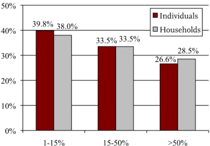
For this sample, the task is to calculate replace-ment rates first for Social Security and then for Social Security and employer-sponsored defined benefit and defined contribution plans, and to present the results for individuals who spent their entire career in the private sector and those who worked in the state-local sector. For those in the public sector, replacement rates are reported by the percent of career spent in that sector: 1-15 percent, 15-50 percent, and more than 50 percent.10_{As shown in Figure 1, roughly one} third of households and individuals are in the middle group, somewhat more in the short-tenure group, and somewhat fewer in the long-tenure group.

Figure 1. Distribution of State and Local Workers by Tenure 39.8% 33.5% 26.6% 38.0% 33.5% 28.5% 0% 10% 20% 30% 40% 50% 1-15% 15-50% >50% Individuals Households

Source: Authors’ calculations from the University of Michi-gan, Health and Retirement Study (HRS) (1992-2008).

The first step is to calculate total earnings just prior to retirement. The HRS restricted data con-tain only the covered earnings records for individual workers. Since earnings are top-coded at the Social Security maximum taxable earnings for each year, the calculation of actual career-average earnings for some individuals requires imputations. For individuals with coded earnings at the cap, their total earnings

(4)

are imputed using regression results from an estimat-ed wage equation.11_{The total earnings history is then} used to calculate the highest five in the last ten years adjusted for inflation for each individual.

The Social Security replacement rate is simply the benefits for the relevant retirement age divided by the calculated pre-retirement earnings. The results are shown in Table 2 below. Social Security alone pro-vides a median replacement rate for private workers of 29 percent and for state-local workers of 26 percent.

The next step is to include income from defined benefit and defined contribution plans. In both cases, income was calculated as the annuitized value of pen-sion wealth. The argument for taking this approach in the case of defined benefit as well as defined contribution plans is that simply reporting the first year benefit would understate the value of state-local defined benefit pensions since these benefits are ad-justed annually – at least partially – for inflation. Both defined benefit and defined contribution wealth come from data posted on the HRS website; these numbers are derived from the restricted pension data provided by the employer. The data are presented at ages 50, 55, 60, 62, and 65, and we selected the observation closest to the individual’s retirement age.12 Unfor-tunately, the wealth data were available only for a portion of our sample, so we had to calculate defined benefit pension wealth from reported benefits for the remaining individuals using the same assumptions about inflation and asset returns.13

Individuals were identified as having a defined contribution plan in one of two ways – either they have defined contribution wealth or they indicated in the first (1992) wave that they were covered by an employer-sponsored defined contribution plan. For

those with coverage but without a measure of defined contribution wealth, IRA balances are set equal to pension wealth because most of the assets in these accounts are rollovers from 401(k) plans and the earn-ings on those rollovers.14_{For those with wealth, IRA} balances are combined with defined contribution as-sets. For those without pension coverage, IRA assets are included in total financial wealth.15

The next step is to derive a stream of annual income by applying annuity factors to the defined benefit and defined contribution wealth. The annuity factors vary by gender and marital status. In addi-tion, an 18-percent increase in cost due to adverse selection, marketing, and other factors is applied to annuities purchased in the private market.16 Mar-ried men are assumed to opt for a joint-and-survivor annuity that provides 50 percent of the benefit to the surviving spouse. The replacement rates reported here are based on nominal annuities, under which the purchasing power of benefits will decline over time; replacement rates based on real (inflation-ad-justed) annuities, which produce lower initial levels of replacement, are reported in the Appendix.

Table 2 shows the impact of income from employ-er-sponsored plans on the replacement rates of single individuals for private sector and state-local work-ers. Adding the annuitized value of defined benefit and defined contribution wealth to Social Security brings the median replacement rate to 42 percent for private sector workers and to 54 percent for workers with some state-local employment. For those with state-local government experience, the replacement rate increases with the percent of career spent in the public sector.17

Table 2. Median Replacement Ratesa_{for Individual Workers by Employment History}

Retirement income source

Private sector State-local sector

All _pensionsWithout _pensionsWith All Percent of career spent in state-local sector

1-15% 15-50% >50 % Social Security 29.2 32.4 27.6 26.4 27.8 26.5 23.4 Social Security + 41.7 32.4 49.1 53.6 46.6 53.3 69.8 pensionsb Addendum: percent 76 35 41 24 10 8 6 of sample

a_{The denominator is the individuals’ top five years of earnings indexed for inflation.}

b_{For those with pension coverage, IRA assets are included in defined contribution wealth; for those without pension}

cover-age, IRA assets are classified as part of financial assets.

(5)

Table 3. Median Replacement Ratesa_{for Households by Employment History}

a. The denominator is the individuals’ top five years of earnings in the last ten years indexed for inflation.

b. For those with pension coverage, IRA assets are included in defined contribution wealth; for those without pension cover-age, IRA assets are classified as part of financial assets.

Source: Authors’ estimates from 1992-2008 HRS.

Household Replacement Rates

Household replacement rates from Social Security are determined by dividing household Social Security benefits calculated at the relevant retirement age by the earnings prior to retirement. Household income from the annuitized value of defined benefit and defined contribution assets (including IRAs for those with defined contribution coverage) is summed for individuals in the households. As before, household replacement rates are estimated at the first year in which both members of the household are retired.18 Dividing these values by the earnings measure pro-duces pension replacement rates.

Replacement rates for households by employ-ment status are shown in Table 3. All the replace-ment rates are slightly higher than those shown for individuals in Table 2, but the pattern remains the same. Replacement rates are higher in the state-local sector than in the private sector, primarily because almost 40 percent of private sector households have no employer-sponsored pension benefits. Within the public sector, replacement rates increase with tenure from 48 percent for households with a short-tenured employee to 72 percent for those with a long-tenured worker. Again, median replacement rates do not reach the 80 percent target for most households with state-local employment.

The Impact of Non-Pension

Financial Assets

The final exercise with the HRS explores the impact of non-pension financial assets on replacement rates. Financial wealth comes from the RAND subset of the HRS and includes stocks, bonds, savings and check-ing accounts, certificates of deposit, and any other account, minus non-housing debt.

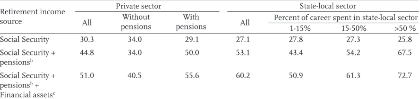
In order to make the calculations economically meaningful, the definition of pre-retirement income needs to be expanded to include a measure of pre-re-tirement income from financial assets. Non-pension financial wealth was not annuitized; rather income was derived by applying a nominal return to asset values. The nominal return on financial assets was 5.1 percent, consistent with the assumptions used throughout the analysis. The results are shown in Ta-ble 4 on the next page. Adding income from financial assets closes the gap somewhat, but still leaves most state-local households short of the 80-percent target.

(6)

Table 4. Median Replacement Ratesa_{for Households, Including Financial Assets, by Employment}

History

1-15% 15-50% >50 % Social Security 30.3 34.0 29.1 27.1 27.8 27.3 25.8 Social Security + 44.8 34.0 50.0 53.1 43.4 54.2 67.5 pensionsb Social Security + 51.0 40.5 55.6 60.2 50.9 61.3 72.7 pensionsb₊ Financial assetsc

a_{The denominator is the individuals’ top five years of earnings in the last ten years indexed for inflation plus income from}

financial assets.

c_{The real return on financial assets is assumed to be 2.3 percent.}

Source: Authors’ estimates from 1992-2008 HRS.

Insights from the Actuarial Data

To provide some insight on why actual replacement rates for workers with state-local experience are lower than generally thought, this section provides evidence on benefit status and replacement rates for those leaving some of the nation’s largest public pension systems in 2010. These systems are CalPERS, Con-necticut SERS, Florida RS, Kentucky TRS, New Jersey PERS, New Jersey TRS, Ohio Schools, Ohio Teachers, Texas ERS, Texas TRS, and Wisconsin RS. Together, these plans represent 18 percent of the nation’s liabili-ties and 22 percent of the members.

First, using each system’s actuarial valuation, it is possible to generate the population of those with at least one year of service who leave public sector employment in a given year, either by quitting before vesting, quitting with deferred benefits, or retiring. The valuations contain data on the demographics of active employees (sex, age, tenure, and salary) and on the probability of retirement – when an employee leaves active service and immediately begins receiv-ing benefits – and of separation – when an employee leaves state-local employment but does not immedi-ately claim benefits because they are not eligible or did not vest. Applying the probabilities of retirement and separation to the population of active members according to their sex, age, and tenure yields the population of those who left state-local active service. Those who leave with under five years of tenure are deemed as not vested. Figure 2 presents the distribu-tion by tenure and benefit status for the 11 large plans identified above.

Figure 2. Distribution of Leavers in Eleven Large Plans by Tenure and Benefit Status, 2011

0% 10% 20% 30% 40% 50% 1-5 5-10 10-15 15-20 20-25 30-35 35-40 40+ Years of service Retirees Deferred vested Non-vested

Note: See endnote 19.

Source: Authors’ estimates from various actuarial reports.

Of those who leave with at least one year of ser-vice, only 32 percent claim benefits immediately, 27 percent will receive a deferred benefit based on their earnings at termination, and 40 percent leave without any promise of future benefits (see Figure 3 on the next page).20

(7)

Figure 3. Percent of Leavers in Eleven Large Plans by Benefit Status

Non-vested, 40.4%

Retirees, 32.2%

Deferred vested, 27.4%

The next step is to estimate replacement rates for those who have left state-local employment. For this exercise, the focus is on a subset of plans where work-ers are covered by Social Security – CalPERS, New Jer-sey PERS, New JerJer-sey TRS, Texas ERS, and Wisconsin RS.21_{In the case of the non-vested, the answer is easy} – the replacement rate is zero.22_{For those who retire} immediately, the calculation is straightforward: the annual benefit divided by the last year’s salary. The annual benefit is calculated by applying the benefit formula to the relevant earnings base, usually the last three years.

For the deferred vested, the benefit calculation is also straightforward: the benefit formula applied to the earnings base in the three years before separa-tion. In order to understand the importance of these deferred benefits at retirement, however, it is neces-sary to compare them with earnings at that time. This calculation requires some assumptions. First, we assume that the separator will claim his benefit at the system’s normal retirement age, generally around age 60. Second, we apply each system’s salary growth assumption to estimate the separator’s salary at that age. Since the average age of those with deferred benefits is 44 (see Table 5), the value of these benefits is seriously eroded by inflation and salary growth.

Table 5. Age and Tenure of Leavers by Benefit Status, 2011

Characteristics Non-vested Deferred benefit Retired

Average age 37.7 44.3 61.0

Average tenure 2.2 11.7 22.8

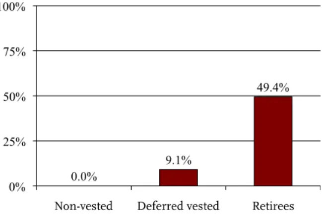
The average replacement rates for those with non-vested, deferred, and immediate benefits by tenure are presented in Figure 4. Those who leave without vesting usually receive only a refund of their contribu-tions with modest interest and no benefits from the plan. Those who leave mid-career receive deferred benefits that amount to less than 10 percent of earn-ings at retirement. And those who claim immediately around age 60 receive benefits equal to 49 percent of final earnings. These differentials are roughly consis-tent with the patterns that emerge from the HRS data.

Figure 4. Replacement Rates for State-Local Workers by Benefit Status

0.0% 9.1% 49.4% 0% 25% 50% 75% 100%

Non-vested Deferred vested Retirees

(8)

Conclusion

This study addresses the widespread perception that state-local workers have more than adequate income in retirement. The perception is consistent with mul-tiplying the 2-percent benefit factor in most plan for-mulae by a 35- to 40-year career and adding a Social Security benefit. But this calculation assumes that individuals spend enough of their career in the public sector to produce such a retirement outcome. Analy-sis of replacement rates of state-local workers in the HRS suggest that households with even long-career state-local employees fall short of the target replace-ment rate of 80 percent of pre-retirereplace-ment earnings.

The explanation for these lower-than-anticipated replacement rates is twofold. First, as the actuarial data show, only 32 percent of workers who leave state-local employment each year claim an immediate benefit. These individuals have more than 20 years of service on average and receive a benefit equal to 49 percent of their pre-retirement earnings. But another 27 percent leave state-local employment with a de-ferred benefit based on their earnings at termination, which will decline in value between termination and claiming as wages and prices rise, so it will amount to less than 10 percent of their projected earnings at retirement. And 40 percent leave without any prom-ise of future benefits. Second, most households with a state-local worker contain a person employed in the private sector, and replacement rates for private sector workers are considerably lower since many end up with nothing more than Social Security.

(9)

Endnotes

1 Munnell et al. (2011).

2 According to our calculations from the HRS, of married couples with a state-local worker, 23 percent include two state-local workers, 58 percent include a state-local and a private-sector worker, and 19 per-cent include a state-local worker and a non-worker. Roughly 40 percent of private sector households rely only on Social Security and receive no employer-spon-sored pension.

3 Technically people are interested in smoothing marginal utility, not consumption. To the extent that they get pleasure from leisure in retirement, they may maintain overall utility with lower levels of consumption after they stop working. The enjoyment of leisure may explain what the literature calls the “retirement-consumption puzzle” – namely, the fact that consumption appears to drop as people retire. See Bernheim, Skinner and Weinberg (2001); Banks, Blundell and Tanner (1998); and Hurd and Rohwed-der (2003).

4 In an extension of the replacement rate approach to test whether people are saving optimally for retire-ment, two recent studies (Engen, Gale, and Uccello (1999) and Scholz, Seshadri, and Khitatrakun (2004)) compare people’s actual behavior with the behav-ior that comes out of simulation models. In these simulations, households attempt to smooth their consumption over their remaining lives as they are buffeted by shocks to their wages, employment, and health. Because of these shocks, households with very similar characteristics can end up with very dif-ferent levels of wealth. These simulations have gener-ally produced results where households’ actual levels of preparedness look very much like the numbers generated by the simulations, suggesting that people respond rationally to life’s events.

5 The percent of Social Security benefits subject to personal income taxation is as follows. Individu-als with “combined income” between $25,000 and $34,000 include 50 percent of benefits; over $34,000 they include 85 percent. Couples with “combined income” between $32,000 and $44,000 include 50 per-cent of benefits; over $44,000 they include 85 perper-cent. “Combined income” is adjusted gross income as re-ported on tax forms plus nontaxable interest income plus one half of Social Security benefits.

6 For an array of pre-retirement earnings levels, they calculate federal, state, and local income taxes and Social Security taxes before and after retirement. They also use the Bureau of Labor Statistics Consumer Expenditure Survey to estimate consumer savings and expenditures for different earnings levels.

7 In the case of retirement, the AIME is determined in two steps. First, the worker’s annual taxable earn-ings after 1950 are updated, or indexed, to reflect the general earnings level in the indexing year, which is age 60. Earnings in years after 60 are not indexed but instead are counted at their actual value. A worker’s earnings prior to age 60 are indexed by multiplying them by the ratio of the average wage in the national economy for the indexing year to the corresponding average wage figure for the year to be indexed. Sec-ond, the AIME is calculated by taking the highest 35 years of wage-indexed earnings between ages 22 and 62 and dividing that total by the number of months in that period.

8 See Juster and Suzman (1995) for a detailed over-view of the survey.

9 The HRS expanded the sample dramatically in 1998 and 2004, with the addition of the War Babies (born between 1942 and 1947) and Early Boomers (born between 1948 and 1953), respectively. The lat-est sample addition, made in 2010, was the inclusion of the Mid Boomers (born between 1954 and 1959). Like the original sample, these three additional co-horts are interviewed every two years.

10 For couples with two state-local workers, the household is classified by the tenure of the longest tenure worker.

11 About 15 percent of the final sample of individuals used in this study required imputations for at least one year of earnings. To impute earnings for those at the maximum taxable earnings, a random-effects, Tobit regression is applied to all of the available data, with earnings below the cap as the dependent variable. The explanatory variables include age, age squared, categorical variables for gender, college de-gree and race, and dummies for each decade. 12 A small fraction (about two percent) of respon-dents in the HRS sample indicated having a pension plan with both defined benefit and defined contribu-tion characteristics. Data on defined contribucontribu-tion

(10)

assets in these “combined” plans were often not available, so they are grouped together with defined benefit plans.

13 The resulting numbers for both defined contri-bution and defined benefit plans are comparable to those reported by Gustman and Steinmeier (1999).

14 Increasingly, of course, IRA accumulations will also include rollovers from defined benefit and cash balance plans.

15 Median defined contribution wealth for those with coverage is $67,000 (excluding IRA assets) and me-dian defined benefit wealth is $97,000. These results are fully consistent with those from other studies. 16 Premium loads on annuities vary with annuity type and with the age of purchase. They also vary between companies and over time, and are somewhat sensitive to the choice of interest rate used to calculate expected present values. Mitchell et al. (1999), Table 3, report loads that are typically on the order of 18 percent.

17 The HRS reports the year that the individual began work in the state-local sector, and the year that state-local employment ended. Subtracting one year from the other provides the total years spent in the state-local sector; those years are then divided by the total length of the individual’s career, as reported in the RAND data.

18 This calculation is done by estimating the annu-ity value for defined benefit and defined contribution pensions for each member of the household starting at his or her retirement age and then projecting this value to the year in which the second member of the household retires.

19 New Jersey PERS and TRS are different from most plans. For most plans, the vesting period is five years. For New Jersey PERS and TRS, the vesting re-quirement depends on the type of retirement. Those who leave service before the normal retirement age must have ten years of tenure in order to claim a de-ferred benefit. Those who retire directly from active service at the normal retirement age have no mini-mum tenure requirement. These provisions result in a small number of retirees with less than five years of tenure, and some non-vested separators with over five years of tenure.

20 This pattern is similar to that found by the State of Maine Unified Retirement Plan Task Force (2010). 21 Connecticut SERS and Florida RS are omitted due to insufficient data.

22 Unlike private sector 401(k) plans, most state and local pensions feature mandatory participation. State-local employees who terminate without vesting in the plan receive a refund on their contributions with a modest rate of interest. Although these refunds are likely quite small, they do have the opportunity to grow over time.

(11)

References

Banks, J., Blundell, R. and S. Tanner, S. 1998. “Is There a Retirement-Savings Puzzle?” American Economic Review 88(4): 769–88.

Bernheim, D., Skinner, J. and S. Weinberg. 2001. “What Accounts for the Variation in Retirement Wealth among US Households?” American Eco-nomic Review 91(4): 832–57.

Engen, Eric, William Gale, and Cori Uccello. 1999. “The Adequacy of Retirement Saving.” Brookings Papers on Economic Activity 2: 65-165.

Gustman, Alan and Thomas Steinmeier. 1999. “Ef-fects of Pensions on Savings: Analysis with Data from the Health and Retirement Study.” Carnegie-Rochester Conference Series on Public Policy 50(June): P271-324.

Hurd, Michael and Susann Rohwedder. 2003. “The Retirement Consumption Puzzle: Anticipated and Actual Declines in Spending at Retirement.” Working Paper 9586. Cambridge, MA: National Bureau of Economic Research.

Juster, F. Thomas and Richard Suzman. 1995. “An Overview of the Health and Retirement Study.” Journal of Human Resources 30(Supplement): pp. S7-S56.

Mitchell, Olivia S., James M. Poterba, Mark J. War-shawsky, and Jeffrey R. Brown. 1999. “New Evi-dence on the Money’s Worth of Individual Annui-ties.” American Economic Review 89(5): 1299-1318. Munnell, Alicia H., Jean-Pierre Aubry, Josh Hurwitz, and Laura Quinby. 2011. “How Prepared Are State and Local Government Workers for Retirement?” Working Paper 2011-15. Chestnut Hill, MA: Cen-ter for Retirement Research at Boston College. Palmer, Bruce A. Palmer. 2008. “2008 GSU/AON

RE-TIRE Project Report.” Research Report Series No. 08-1 (June). Atlanta, GA: J. Mack Robinson College of Business, Georgia State University.

Scholz, John Karl, Ananth Seshadri, and Surachai Khitatrakun. 2004. “Are Americans Saving ‘Op-timally’ for Retirement?” Working Paper 10260. Cambridge, MA: National Bureau of Economic Research.

State of Maine Unified Retirement Plan Task Force. 2010. Task Force Study and Report: Maine State Employee and Teacher Unified Retirement Plan. Augusta, ME.

University of Michigan. Health and Retirement Study (HRS), 1992-2008. Ann Arbor, MI.

(12)

(13)

Replacement Rates Calculated on the Basis of Inflation-Adjusted

Annuities

Table A1. Median Replacement Ratesa_{for Individual Workers by Employment History}

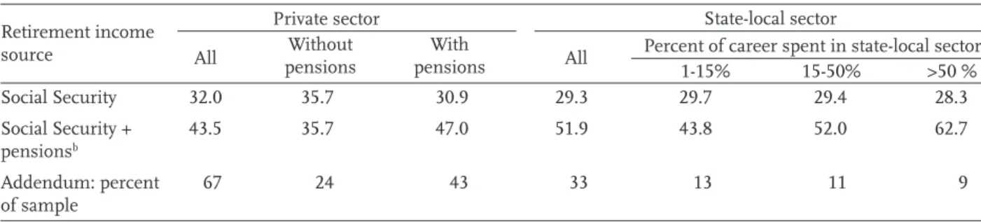
Table A2. Median Replacement Ratesa_{for Households by Employment History}

Table 4. Median Replacement Ratesa_{for Households, Including Financial Assets, by Employment}

History

1-15% 15-50% >50 % Social Security 30.3 34.0 29.1 27.1 27.8 27.3 25.8 Social Security + 41.5 34.0 44.6 48.3 40.6 48.9 58.3 pensionsb Social Security + 47.3 40.5 50.3 55.3 48.0 54.9 66.4 pensionsb₊ Financial assetsc

a_{The denominator is the individuals’ top five years of earnings indexed for inflation.}

c _{The real return on financial assets is assumed to be 2.3 percent.}

(14)

About the Center

The Center for Retirement Research at Boston Col-lege was established in 1998 through a grant from the Social Security Administration. The Center’s mission is to produce first-class research and educational tools and forge a strong link between the academic com-munity and decision-makers in the public and private sectors around an issue of critical importance to the nation’s future. To achieve this mission, the Center sponsors a wide variety of research projects, transmits new findings to a broad audience, trains new schol-ars, and broadens access to valuable data sources. Since its inception, the Center has established a repu-tation as an authoritative source of information on all major aspects of the retirement income debate.

Affiliated Institutions

American Enterprise Institute The Brookings Institution

Massachusetts Institute of Technology Syracuse University

Urban Institute

Contact Information

Center for Retirement Research Boston College Hovey House 140 Commonwealth Avenue Chestnut Hill, MA 02467-3808 Phone: (617) 552-1762 Fax: (617) 552-0191 E-mail: crr@bc.edu Website: http://crr.bc.edu

© 2011, by Trustees of Boston College, Center for Retirement Research. All rights reserved. Short sections of text, not to exceed two paragraphs, may be quoted without explicit permission provided that the authors are identified and full credit, including copyright notice, is given to Trustees of Boston College, Center for Retirement Research.

The CRR gratefully acknowledges Great-West Retirement Services for its support of this research. The opinions and conclusions expressed in this brief are solely those of the authors and do not represent the opinions or policy of the CRR or Great-West Retirement Services.