Dynamic Load Balancing in CP2K
Pradeep Shivadasan
August 19, 2014
MSc in High Performance Computing The University of Edinburgh
Abstract
CP2K is a widely used atomistic simulation package. Unlike other similar packages, CP2K uses the Quickstep algorithm for molecular dynamics simulation. Quickstep is an improvement over plane-wave implementation of DFT and uses a dual-basis approach to store data in different representation −wave functions are stored as sparse matrix and electronic density stored on distributed regular grids. A frequent conversion between the different representation is needed to find the ground state energy. A load balancing module is available in CP2K which optimizes the mapping of tasks to processes during the conversion from matrix to regular grids format. However, the module allocates O(P2) memory, where P is the number of MPI processes, and uses a serial algorithm to optimize load on all processes. The high memory requirement and serial load balancing task limits the scalability of the algorithm to high number of processors. This document describes a solution to the high memory requirement problem and shows the issues in parallelizing the serial load balancing task.
Contents
1 Introduction 1
2 Background 2
2.1 MPI . . . 2
2.2 Algorithm analysis framework . . . 4
2.2.1 Levels of parallelization . . . 4
2.2.2 Dependency Analysis . . . 6
2.3 Test data . . . 9
3 An overview of load balancing in CP2K 9 3.1 task data-structure initialization . . . 13
3.2 The list data-structure . . . 13
3.3 Load optimization . . . 14
3.4 Update task destination . . . 20
4 Issues with current implementation 20 4.1 High memory requirement . . . 20
4.2 Serial task . . . 22
5 Improvements 23 5.1 Resolving memory issues . . . 23
5.1.1 Computing global load . . . 24
5.1.2 Update local load list . . . 25
5.1.3 Parallel solution . . . 32
5.1.4 Checking program correctness . . . 33
5.1.5 Performance measurement . . . 37
5.2 Resolving serialization issues . . . 38
5.2.1 Existing implementation . . . 38
5.2.2 Algorithm analysis . . . 41
5.2.3 Parallel Implementation . . . 43
5.2.4 Checking program correctness . . . 48
5.2.5 Result comparison . . . 49
5.2.6 Performance measurement . . . 51
6 Retrospective 53 6.1 Project Goals and Objectives . . . 53
6.2 Major Milestone Achievement . . . 53
6.3 Risk Management . . . 54
6.4 Lessons Learnt . . . 54
7 Conclusions 56
List of Figures
1 Conversion between representations. . . 1
2 MPI communication modes . . . 3
3 5 stage pipeline . . . 4
4 SIMD architecture . . . 5
5 Task parallelism . . . 6
6 Data Dependency Scenarios . . . 8
7 Mapping of tasks on grid . . . 11
8 Cost model accuracy . . . 12
9 Flowchart of the load balance optimization process. . . 12
10 Example layout of the 3 dimensional list array . . . 14
11 Possible network arrangements . . . 15
12 Iterative load sharing . . . 17
13 Calculating global load - in serial . . . 18
14 Update list array . . . 21
15 High memory requirement warning in distribute_tasks routine . . . 22
16 Out of memory warning in optimize_load_list routine . . . 22
17 Memory needed vs number of processes . . . 23
18 Computing global load - in parallel . . . 26
19 Data Dependency Analysis . . . 27
20 Data Dependency Graph . . . 28
21 Data Dependency Graph with self dependency on S1 removed . . . 29
22 Data Dependency Analysis after loop transformation . . . 31
23 Data Dependency Graph after loop transformation . . . 31
24 Final parallel algorithm. . . 35
25 Sample assertion failure report produced by CPPrecondition function. . 36
26 Comparison of old vs new implementation . . . 38
27 Flowchart for global load optimization process . . . 39
28 Algorithm execution patterns . . . 43
29 Global load calculation - New method . . . 45
30 Output of CP2K regression test utility . . . 49
31 Performance comparison of the serial and the parallel load balancing algorithm. . . 50
32 Speedup of parallel implementation . . . 51
33 Parallel efficiency . . . 52
34 Profiler Output . . . 53
35 Risk impact matrix . . . 55
List of Algorithms
1 Compute load list . . . 16
2 Optimize load list . . . 19
3 Computation of global load . . . 24
4 Parallel computation of global load . . . 25
5 Global load distribution . . . 26
5a Parallel inner-loop . . . 30
5b Parallel outer-loop . . . 32
6 Final implementation . . . 33
7 Compute flux limits . . . 40
7a Find optimum flux . . . 41
7b Update global load . . . 42
8 Parallel computation of global load . . . 44
9 Compute parallel flux limits . . . 46
9a Parallel load optimization . . . 47
Acknowledgements
If I have seen further it is by standing on the shoulders of giants
Newton, 1675 I would like to express my deepest gratitude to my supervisor, Iain Bethune (EPCC), for his excellent guidance, patience, and encouragement in carrying out this project work.
1
Introduction
CP2K [1] is an open-source tool for atomistic simulation available under the GNU General Public License (GPL). It provides a broad range of models and simulation methodologies for large and condensed phase systems. The software is written in For-tran95 and parallelized for distributed memory architectures using MPI augmented with OpenMP for shared memory architectures. It uses various libraries like dense linear algebra packages (BLAS, LAPACK, ScaLAPACK); fast fourier transforms (FFTW); specialized chemical libraries like electron repulsive integrals (libint) and exchange cor-relation functionals (libxc) to decrease the complexity and enchance the efficiency and robustness of the code.
CP2K is mainly used to explore properties of complex systems. The methods avail-able in CP2K to explore the potential energy surface areStationary Points- to optimize atomic positions and cell vectors based on various algorithms like cubically scaling methods, Hessian and linear scaling methods;Molecular Dynamics- DFT based molec-ular dynamics simulation to simulate atoms and molecules in a system; Monte Carlo -alternative to MD for sampling purposes;Ehrenfest dynamics- to study the time depen-dent evolution of electric fields in a system and the response of the electronic structure to perturbation; andEnergy and force methods- to model materials usingClassic Force FieldsandElectronics Structure Methods. See [2] for examples of outstanding science performed with CP2K.
CP2K uses the Quickstep [3] algorithm, an efficient implementation of density function theory (DFT) based molecular simulations method. It uses a dual-basis approach where data is stored in two distinct representations - wave-functions stored in a sparse matrix and electronic density stored on distributed regular grids. Sparse matrix storage uses less memory and is faster to process while distributed regular grid helps in computing Hartree potential efficiently. However, the disadvantage of this representation is that to find the ground state energy of the system, the data needs to be converted between these two representations in every iteration of the Self-Consistent field (SCF) loop.
Figure 1 shows the conversion between various representations. The conversion from matrix to regular grids is called Collocation and the reverse conversion is called Inte-gration.
As mentioned earlier, the conversion between various representation is carried out in every iteration of the SCF loop hence it needs to be very efficient. A number of perfor-mance improvements, including matrix to regular grid conversion; FFT methods; load balancing of tasks transferred from real-space to planewave representation, were made to improve the performance of the Quickstep algorithm in dCSE [4] project.
The scope of this project is to improve the scalability of the existing load balancing algorithm by reducing its memory requirements and parallelizing the algorithm. The rest of the document describes the efforts to improve the existing load balancing module. Section 2 provides an overview of the tools and technologies used to ana-lyze and develop an improved solution for the problem. Section 3 describes the data-structures and algorithms used to implement the load balancing module. Section 4 lists the limitations of the existing implementation followed by a discussion of the new im-proved solutions in Section 5. Section 6 summarizes the lessons learned during the project development. Finally, Section 7 summarizes the work carried out during the project.
2
Background
CP2K version 2.4.0 was used for the development of the solution. The solution was developed on ARCHER [5] (Advanced Research Computing High End Resource), the UK National Supercomputing Facility. The ARCHER facility is based around a Cray XC30 supercomputer with 1.56 petaflops of theoretical peak performance. It consists of 3,008 nodes with each node having two 12-core 2.7 GHz Ivy Bridge multicore pro-cessors for a total of 72,192 cores. Each node contains 64 GB of DDR3 main memory, giving 2.6 GB of main memory per core. The nodes are interconnected via an Aries Network Interface Card. See [6] for full details of the system.
A brief overview of the tools and techniques used to develop the solution follows.
2.1
MPI
The Message Passing Interface (MPI) [7] is a message passing library used to program parallel computers mostly distributed memory system. MPI is a SPMD (Single Program Multiple Data) style of parallel programming where data is communicated between pro-cesses using messages. MPI provides two modes of communication: a) Point-to-point; and b) Collective . Point-to-point operation involves message passing between two different processes. One performs a send operation and the other process performs a matching receive operation. A collective communication involves all processes within the system. Collective operations are used for synchronization, data-movement (broad-cast, scatter/gather, all to all), and reduction operations (min, max, add, multiply, etc). Figure 2 shows modes of MPI communication diagrammatically. Parallel algorithms in CP2K are based on message passing using MPI.
0 1 2 3
(a) Point-to-point communication
1 2 3
0
(b) Collective communication
Figure 2: MPI communication modes. a) is a point-to-point communication between two processes. b) is a collective communication where the final result is available on a single process. Another form of collective communication is available where the result is made available on all processes in the group.
2.2
Algorithm analysis framework
2.2.1 Levels of parallelizationA modern processor provides support for different levels of parallelism at instruction level, data-level, and task level. The tools and techniques to exploit parallelism are different at different levels. The next sections provide a brief overview of parallelism support in a modern processor and techniques to exploit the available parallelism.
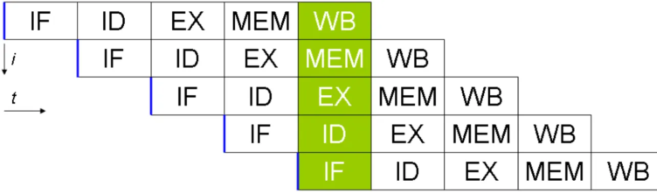
Instruction Level Parallelism or Pipeline Parallelism
A modern processor provides multiple ways to execute program instructions in paral-lel to reduce the program execution-time. Instruction Level Paralparal-lelism [8] (ILP) or Pipeline Parallelism is a technique where multiple independent instructions are exe-cuted simultaneously in a pipelined manner. Modern processors contain multi-stage pipelines where micro-instruction are executed in parallel. Figure 3 shows a 5 stage pipeline where a new independent instruction can start execution every cycle (provided the resources needed by the instruction are available). It is imperative that the proces-sor pipeline is issued new instructions on every clock cycle for efficient utilization of the processor. Independent instructions keep the pipeline busy and increase the pro-cessor performance, while dependent instructions stall the pipeline and reduce the per-formance. Optimizing compilers are good at exploiting ILP by finding independent instructions and scheduling them efficiently to execute in parallel. Another method to exploit ILP in software is loop unrolling which directly exposes independent operations to the compiler.
Figure 3: A 5 stage pipeline where an instruction is executed in stages and a new in-struction can start execution as soon as the resource used by the last inin-struction becomes available. The stages shown in the diagram are Instruction Fetch (IF), Instruction De-code (ID), Execute (EX), Memory (MEM), and Write Back (WB). Source [13].
Data-Parallelization or Vectorization
Modern hardware provides vector units to exploit level parallelism [9]. In data-parallelization, a single instruction is used to perform the same operation on multiple
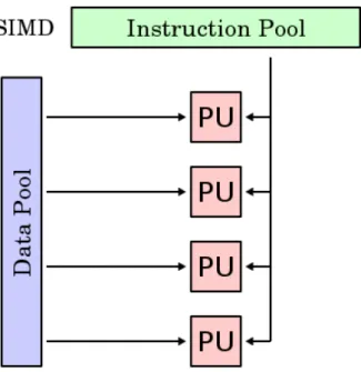
data points simultaneously. Vector units uses special instruction set called SIMD [10] (Single Instruction Multiple Data) instructions. SIMD instructions include instructions to perform arthimetic, data-movement, and bit-wise operations for both integer and floating point values. Some examples of SIMD instructions from different vendors are SSE, AVX from Intel; 3DNow! from AMD; AltiVec, SPE from IBM; MAX from HP; and NEON from ARM.
The vector instructions perform better than a SISD (Single Instruction Single Data) instruction due to the fact that only a single instruction is decoded and executed for multiple data points. The data access pattern also exhibits a strong locality of refer-ence. The data is accessed from consequent memory locations. This predictable pattern helps the hardware to prefetch data before the instruction requires it. Many optimiz-ing compilers are capable of producoptimiz-ing automatic vectorized code. These compilers checks for data dependencies between instructions and vectorize parts of code that are independent. Figure 4 shows a SIMD instruction working on multiple data points.
Figure 4: A SIMD architecture with multiple Processing Units (PU) processing multiple data points using a single instruction. Source [14].
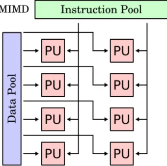
Task Parallelism
Task parallelism [11] is used to execute independent tasks in parallel. Independent task could be a print job working in the background and windows updating in the foreground. Independent task could also be iterations of a loop executing in parallel. Independent task could be executed on the same machine or on distributed machines. Tasks are cre-ated by Threads or Processes, abstractions provided by the operating system. They are optimally scheduled by the operating system to utilize the available resources. Hard-ware support for tasks are provided by multiple or multi-core processors. Operating
systems uses the concept of time-slicing where a single CPU is multiplexed between multiple Threads and Processes.
In performance programming, tasks are mostly iterations of loop running in parallel or program running on distributed systems. On a shared memory machine, OpenMP [12] is mostly used to parallelize iterations of a loop. Other commonly used threading li-braries are pthreads, Win32 threads, Boost etc. On a distributed cluster environment, the two typical approaches to communication between cluster nodes have been PVM, the Parallel Virtual Machine and MPI, the Message Passing Interface. However, MPI has now emerged as the de facto standard for message passing on a distributed environ-ment.
Compared to SIMD instruction, a thread or a process executes a MIMD (Multiple In-struction Multiple Data) type of inIn-struction. Figure 5 shows a MIMD inIn-struction work-ing on multiple instructions and multiple data points.
Figure 5: A MIMD architecture (Task parallel) with multiple Processing Units (PU) processing multiple data points using multiple instructions. Source [15].
2.2.2 Dependency Analysis
As shown in the Section 2.2.1, modern processors executes programs faster by execut-ing instructions in parallel. Instructions can only be executed in parallel if there are no execution-order dependency between statements/instructions. Dependent instructions inhibit parallelism and may introduce bubbles in the processor pipelines or serialize loop iterations. Dependency analysis techniques are available to check for dependen-cies between instructions and loops. The next sections discuss techniques available to check fordata dependenciesandloop dependenciesin a program.
Data Dependence Analysis
Understanding data dependencies is fundamental in implementing parallel algorithms. Data Dependence Analysis [17] determines whether or not it is safe to re-order or par-allelize statements. Bernstein’s conditions [18] describe when the instructions are inde-pendent and can be executed in parallel.
O(i)∩I(j) =∅ (1)
I(i)∩O(j) =∅ (2)
O(i)∩O(j) =∅ (3) Where:
O(i): is the set of (output) locations altered by instructioni I(i): is the set of (input) locations read by instructioni
∅: is an empty set.
A potential data-dependency exists between instruction i and a subsequent instruction j when at least one of the conditions fails.
A flow dependency (statement using results produced by its preceding statements) is introduced by the violation of the first condition. Ananti-dependencyis represented by the second condition, where the statementj produces a variable needed by statementi. The third condition represents anoutput dependency: When two statements write to the same location, the result comes from the logically last executed statement.
Figure 6 demonstrate several kinds of dependencies. In Figure 6(a), statement S2 cannot be executed before (or even in parallel with) statement S1, because statement S2 uses a result from statement S1. It violates condition 1, and thus introduces a flow dependency. Similarly, Figure 6(b) and Figure 6(c) violates condition 2 and condition 3 respectively. Table 1 shows the notations used in this document to describe data dependencies be-tween statements.
Flow dependence δ
Anti-dependence ¯δ
Output dependence δ◦
S1 :X = S2 : = X
(a) Flow or true dependency
S1 : = X S2 :X = (b) Anti dependency S1 :X = S2 :X = (c) Output dependency
Figure 6: Data Dependency Scenarios. a) shows X cannot be read in statement 2 until X is written to in statement 1. b) shows X cannot be written to in statement 2 until statement 1 has read the value in X. c) shows X cannot be written to in statement 2 until X is written to in statement 1.
Loop Dependency Analysis
A numerical application spends majority of its time executing instructions inside a loop. Hence, loops are potential candidates for parallelization. A well-designed loop can pro-duce operations that can all be performed in parallel. However, a single misplaced dependency in the loop can force it all to be run in serial. A Loop Dependency Analy-sis [17] is the task of determining whether statements within a loop body form a depen-dence, with respect to array access and modification. If the analysis can determine that no data dependencies exist between the different iterations of a loop then the iterations can be executed in parallel. The types of dependencies in loops are:
1. Loop-independent dependence. 2. Loop-carried dependence.
Loop-independent dependenceoccurs between accesses in the same loop iteration, whereas
loop-carried dependence occurs between accesses across different loop iterations. List-ing 1 shows example of loop dependencies.
DO I = 1 , N
S1 : A( I ) = A( I−1) + 1 S2 : B ( I ) = A( I )
ENDDO
In the given example, there is loop-carried dependence from statementS1ito statement
S1i+1. That is, the instruction that uses A(i-1) can only access the element after the
previous one computes it. Every iteration depends on the result of its previous iteration. Clearly, this is not a problem if the loop is executed serially, but a parallel execution may produce a wrong result. Similarly, there is a loop-independent dependency between statements S1i and S2i. The statement S2i depends on the output of statement S1i
hence the statements cannot be re-ordered or executed in parallel.
Another concept that is important in loop analysis is the Data Dependency Direction Vector. As the name suggests, direction vectors return the direction of the dependency: forward, backward or equal. In forward dependency the value is computed in iteration
iand used in iterationi+k. In backward dependency the vale is computed in iteration
i and used in iteration i-k. This is only possible in nested loops. Finally, in equal dependency the value is computed in iterationiand used in iterationi. These techniques will be examined in greater detail in the coming sections.
Table 2 shows the notations used in this document to show direction of loop dependency. Forward <
Backward >
Equal =
Table 2: Data dependency direction notations
2.3
Test data
The two test inputs used to check the performance and correctness of the modified algorithms are H2O-32 and W216. H2O-32 is a small benchmark which performs 10 MD steps on a system of 32 water molecules in a 9.85 Angstrom cubic cell. This small benchmark is used to quickly check the performance and correctness of the modified algorithms.
W216 is a large system of 216 molecules in a non-periodic 34 Angstrom cell. The atoms in the system are clustered in the center of the simulation cell. Because of large molecules some systems will have fewer tasks than others. This creates a load imbal-ance and is a good test case for testing the load balancing algorithm.
3
An overview of load balancing in CP2K
As discussed in the introduction section, CP2K uses Quickstep algorithm for molecular simulations. This algorithm uses dual basis approach and represents data in two differ-ent formats: sparse matrix and regular grid. The data needs to be converted between
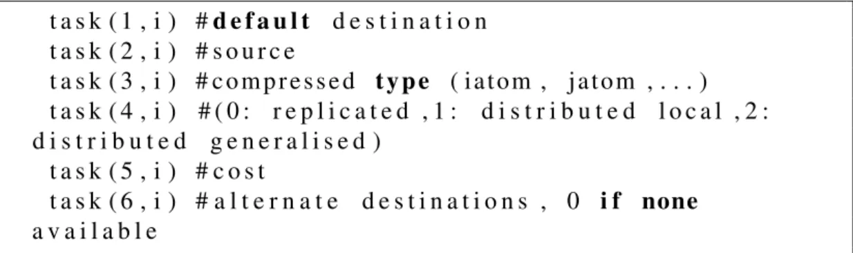
these two representations in every iteration of the SCF loop. Figure 1 shows the con-version between different representations. During the concon-version, the gaussian basis function stored in the sparse matrix form is distributed to the real-space grid (shown as the collocation step in Figure 1). The gaussian basis function is stored as a task list in the source process. Once distributed, the task may be executed by other process in the system. The function of the load balancing module is to optimize the choice of the destination process to balance the load of task across all processes in the system. The load balance is achieved by migrating tasks between the least loaded neighboring processes. The key information to migrate tasks between processes are the default desti-nation process of a task, its alternative destidesti-nations, and the cost of the task. The default destination of a task is the process where it will be executed. The alternate destinations are the processes where the task may be migrated for load balancing. Figure 7 shows the mapping of task destination and its alternate destinations on the real-space grid. The task is represented by thetaskdata-structure in CP2K. Listing 2 shows the fields of this data-structure. t a s k ( 1 , i ) #d e f a u l t d e s t i n a t i o n t a s k ( 2 , i ) # s o u r c e t a s k ( 3 , i ) # c o m p r e s s e d t y p e ( i a t o m , j a t o m , . . . ) t a s k ( 4 , i ) # ( 0 : r e p l i c a t e d , 1 : d i s t r i b u t e d l o c a l , 2 : d i s t r i b u t e d g e n e r a l i s e d ) t a s k ( 5 , i ) # c o s t t a s k ( 6 , i ) # a l t e r n a t e d e s t i n a t i o n s , 0 i f none a v a i l a b l e
Listing 2: Fields of the task data-structure. The alternate destinations field also contains the process ID of the default destination process.
As shown in Listing 2, the default destination is stored in task(1,i)field, the al-ternate destinations are stored in task(6,i)field, and the cost of the task is stored in task(5,i) field. The destination and the alternate destinations of the task are computed in thers_find_noderoutine. The cost of a task is computed as
((lmax+v1)∗(cmax+v2)3∗v3∗f raction+v4 +v5∗lmax7)/1000
Where:
cmax: measure of the radius in grid points of the gaussian
lmax: angular momentum quantum orbital for the particular gaussian
f raction: factor to split cost between processes for the generalized task type
vi: constant to account for other costs
Figure 8 shows accuracy of prediction of the cost model.
Figure 9 shows the flowchart summarizing the steps to optimize load balance between all processes. Every process maintains a list of tasks that it is responsible to execute, along with a list of alternate destinations where the task can be migrated for load balanc-ing. The idea of load balancing is to shift tasks to their least loaded alternate destination
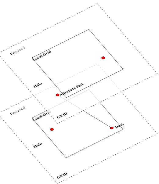
Process 0 Dest. Local Grid Halo GRID Process 1 Alter nate dest. Local Grid Halo GRID
Figure 7: Mapping of tasks on grid. Tasks are shown as red circles. A tasks default process is the one where it falls within the local grid. Alternate destinations are the process where the entire task falls within the halo region.
and even out load among all processes. The load of a process is calculated by summing the cost of the tasks that is assigned to it. Once the load on each process is calculated, the optimum load of all processes is found by iteratively shifting the load between the destination and alternate destination processes. Finally, the task is re-assigned to its least loaded possible destination.
The load balancing module is implemented in thetask_list_methods.f90 file.
load_balance_distributedis the driver routine that implements the load bal-ancing process. The driver routines callscreate_destination_list to allocate memory for thelistdata-structure (discussed in Section 3.2),compute_load_list
to add task load to thelist data-structure (discussed in Section 3.2) and update task destination after load optimization (discussed in Section 3.4), andoptimize_load_list
Figure 8: Cost model accuracy. Source [16].
The next sections show details of the implementation begining with the key data-structures used in the implementation.
Start
Compute destination, alternate destinations, and cost of tasks
Calculate load on processes
Optimize load
Reassign tasks to the least loaded process in their destination list
Stop
3.1
task data-structure initialization
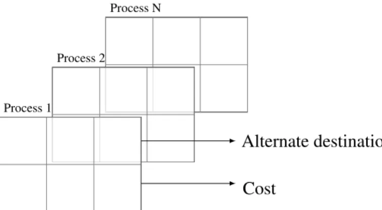
As discussed in the previous section, thetask data-structure contains the key infor-mation to migrate tasks between processes to optimize the load on every process. The task’s default destination and alternate destinations are found on the real space grid. The real space grid is decomposed into chunks (Grid) handled by different MPI processes. The default destination of the task is the process which have sections of the grid, in-cluding halos, that fully contain the grid-points required to process the current gaussian (task). Then the 6 neighbour nodes (+/- x,y,z) are checked to see if they fit the bounds of the task. If so these processes are set as the alternate destinations of the task. See Figure 7 for a 2D view of the task mapping process. See [4] for a detailed discussion of the grid layout.
The information stored in thetaskdata-structure is re-organized and stored as a map of task destination, alternate destinations and its cost. This new re-organized information is stored in a data-structure called list. The next section describes the list data-structure in detail.
3.2
The list data-structure
As discussed in the previous section, the list data-structure stores the re-organized information of thetaskdata-structure. From now onwards, the default task destination will be referred to as the source process and the alternate task destinations will be re-ferred to as the destination process. The term cost and load will be used interchangeably to refer to the load of the process.
Thelist data-structure is a 3 dimensional array. Figure 10 shows the layout of this data-structure. The Rank (process ID is referred to as Rank in MPI) of the destinations are stored in the first dimension of the array and the cost of the tasks that can be shifted to these destinations are stored in the second dimension. The third dimension is used to index the array for all processes in the system. For example, in an 8 process system, the statement dest = list(1,2,3)returns the rank of the 2nd destination of the
3rd source. Similarly, the statementload=list(2,2,3) returns the cost of task of the same example process. The total load of the source process is the sum of the cost of the task transferable to its destination process.
list initialization
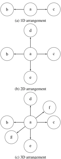
Thelist array is created in the routinecreate_destination_list. The size of the first and second dimension of the array is determined by the number of desti-nations a process has: 3 for 1D decomposition, 5 for 2D decomposition, and 7 for 3D decomposition. The different possible decompositions are shown in Figure 11. The size of the third dimension is determined by the number of processes in the system.
Process N
Process 2
Alternate destinations Cost
Process 1
Figure 10: Example layout of the 3 dimensional list array with the alternate task desti-nations of the process stored in the first dimension of the array and the corresponding task cost stored in the second dimension. The index of the third dimension (shown in the vertical direction) is used as the source process identifier.
first dimension of the listdata-structure with the Ranks of the task destination pro-cesses. The destination process information is found in thers_descsdata-structure. The destination processes are the neighboring process of the source process under con-sideration. Since the information stored inrs_descs is global and same in all pro-cesses, the first dimension values are same in all processes. A detailed discussion of
rs_descsdata-structure is beyond the scope of this document.
The second dimension of thelistis initialized with the cost of the tasks. The cost of the task stored in thetaskdata-structure is added to its destination process cost in the
listdata-structure. The initialization is done in thecompute_load_listroutine. The routine handles two cases: initializelistarray with cost of the task, and reassign task to optimum process after load optimization.
The pseudo-code for computing process load is shown in Algorithm 1. The algorithm groups all tasks into blocks that handles the computation of same atom pairs and thus depend on the same matrix block. A list of destination for every task in the block is created and for each task in the block, its alternative destinations are checked in the list. If alternative destinations are found in the list, the task is assigned to the least loaded destination in the list. Otherwise, the task is assigned to its default destination. This completes the initialization of the list data-structure. Next, using this information, the global load of all process is computed and optimized for load balancing.
3.3
Load optimization
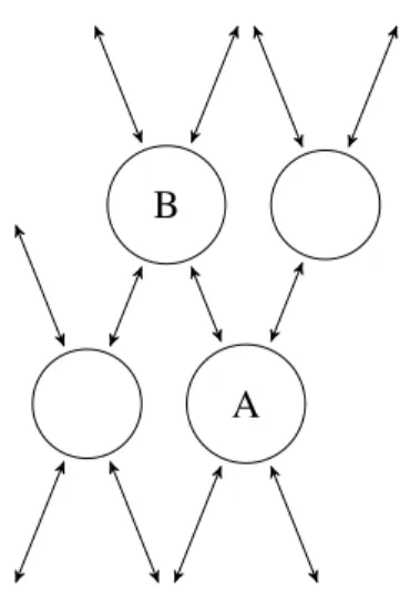
CP2K uses an iterative algorithm for load optimization. The load of processes are optimized and tasks are migrated to their possible destinations to balance the work load across processes. Figure 12 shows the load balancing process diagrammatically. The diagram shows two processes, Process A and Process B as load sharing processes. The process begins by Process A sharing its work load with Process B, Process B in-turn
b a c (a) 1D arrangement b a c d e (b) 2D arrangement b a c d e f g (c) 3D arrangement
Figure 11: Possible network arrangements. a) shows 1D arrangement where load can be shared between processes arranged in x dimension only. b) shows 2D arrangement where load can be shared between processes arranged in x and y dimensions. c) shows 3D arrangement where load can be shared between processes arranged in x, y, and z dimensions.
Algorithm 1Compute load list
Begin
for allblocksintasksdo .task blocks with same atom pairs
for alliinblocksdo destsi ←taski.dest
end for
for alliinblocksdo
for alldintaski.alt_destsdo
ifd∈AN Y(dests)then alt_opts←d
end if end for
ifalt_opts6=∅then
rank← LEAST_LOADED(alt_opts)
else
rank←taski.dest
end if
li←list_index(list, rank)
ifcreate_listthen .Case 1: init list
list(2, li, taski.dest) = list(2, li, taski.dest) +taski.cost
else .Case 2: update task dest
iflist(1, li, taski.dest)6=taski.destthen
iflist(2, li, taski.dest)≥taski.costthen
list(2, li, taski.dest) = list(2, li, taski.dest)−taski.cost
taski.dest←rank
end if end if end if end for end for End
A B
Figure 12: Iterative load sharing
shares its work load with its neighbors. The neighbors of Process B shares their work load with their neighbors and so on. This process is iteratively executed optimizing the load across the system. Once optimized, the tasks are migrated from overloaded process to the least loaded process.
The pseudo-code for load optimization is shown in Algorithm 2. The process is imple-mented in the optimize_global_list routine. The algorithm has three parts: calculate global load, optimize global load, and update local load (the list data-structure). Each part is explained next.
Calculating global load
All process store their task information locally in thelistdata-structure. These frag-mented local load information is accumulated on a single process (Rank 0) and pro-cessed to create the global load information. The global load information shows the total load on each process globally.
Algorithm 2 shows the pseudo-code to compute global load of each process. The local load information from all process is gathered on Rank 0. A temporary array,
load_per_source1, sufficient enough to store information from all processes is allocated to gather this information. The global load on each process is calculated by summing the local load gathered in the last step. The global load is stored in the
list_globalarray.
Figure 13 shows the steps to calculate global load diagrammatically. In the diagram, load of Process P0 and Process P1 is gathered on Process P0 and stored in the temporary arrayload_per_source. The values in the temporary array are added together to find the global load of each process.
1The load_per_source array is declared as a 1D array in the implementation. Here the array is shown as a 2D array for ease of explaination.
B
1B
2B
3P1
B
10B
20B
30P1
A
1A
2A
3P0
P0
A
01A
02A
03P0
P1
(a) Local load information in the list data-structure. Alternate destinations not shown.
A
1A
2A
3B
1B
2B
3A
01A
02A
03B
10B
20B
30P0
X
1X
2X
3Y
1Y
2Y
3+
+
+ + + +(b) Load gathered from all processes to Rank 0. Process wise load added to compute global load Figure 13: Calculating global load - in serial. a) shows load information stored in the list data-structure (alternate neighbors fields excluded from the diagram). b) shows load information gathered on Rank 0 and global load computed serially on Rank 0.
Algorithm 2Optimize load list
Begin
MPI_GATHER(list.load, load_per_source, . . .) .Gather Local loads
ifRAN K = 0then for alliinnP rocdo
for allj innP rocdo
load_allj ←load_allj +load_per_sourcei,j .Calculate global load
end for end for
list_global.dest←list.dest list_global.load←load_all
BALANCE_GLOBAL_LIST(list_global) .Optimize global load
for alliinnP rocdo for allj innP rocdo
tmp←MIN(list_globalj.load, load_per_sourcei,j)
load_per_sourcei,j ←tmp
list_globalj.load ←list_globalj.load−tmp
end for end for end if
MPI_SCATTER(load_per_source, list.load, . . .) .Update local load
End
Optimizing global load
The load optimization algorithm is implemented in the balance_global_list
routine. This algorithm works on the list_global data-structure described previ-ously. It finds the optimum flux (amount of work load) that could be shifted between the source and the destination process. The calculated optimum flux is used to normalize the load stored in thelist_globaldata-structure.
Similar to the list data-structure, the list_global array stores values in pairs of alternate destinations and task load. However, the load information stored in the
list_global array is that of the global load of all processes in the system. This values also sets a limit on the amount of load that could be shifted between the pairs of process. The limit is called the flux limits. Another concept used in the load bal-ancing module is that of a flux connections. The pair of the source and the destination process in thelist_global array forms aflux connections. The load optimization algorithm balances the load on processes by optimizing the load between the pairs in the
flux connections. See Section 5.2.1 for a detailed discussion on the load optimization process.
Updating local load list
The optimized global list, computed in the last step, is used to update the local load stored in the listarray. The new local load is computed by the Rank 0 process and
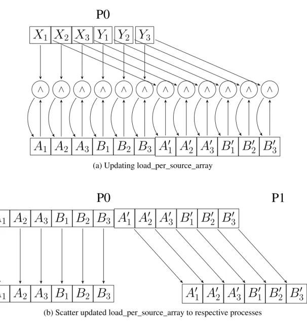
scattered to their respective processes. Processes gather this information and update theirlistarray with the new load information. The pseudo-code for the algorithm is shown in Algorithm 2. The algorithm reassigns local load array (load_per_source) with the minimum of existing values or the newly computed load. The updated load is scattered to the respective processes which updates the load values in theirlist ar-ray. The steps to update the local load information is shown diagrammatically in Figure 14. The diagram shows the updated local load information calculated in Rank 0 and scattered to their respective processes.
3.4
Update task destination
Finally, the updated list is used to reassign tasks to its optimum destinations. The pseudo-code for the task reassignment is shown in Case 2 of Algorithm 1. Thelist
data-structure contains optimized load from the last step. The algorithm searches for the least loaded process in the task’s alternate destination list. If the destination process can accommodate load of the task, the task is assigned to the process otherwise the task remains with its default process.
This concludes the discussion on existing implementation of the load optimization pro-cess. The next section discusses issues with the current implementation followed by solutions to the identified issues.
4
Issues with current implementation
4.1
High memory requirement
The first major issue with the current implementation is the amount of memory required to implement the load balancing module. The most expensive data-structure in terms of memory requirement is the temporary array load_per_process. Memory for this data-structure is allocated in the optimize_load_listroutine. The variable is used to gather local load information from all processes in the system. The load in-formation is retrieved from thelistdata-structure.listusesO(P)memory to store load information of all task in a process. In order to store this information centrally,
load_per_process allocatesO(P2) amount of memory. The amount of memory
needed is calculated as
sizeof int∗max_dest∗ncpu2
Where:
sizeof int: is the word size on the executing machine
max_dest: is maximum alternate destinations for a task
X
1X
2X
3Y
1Y
2Y
3P0
A
1A
2A
3B
1B
2B
3A
01A
02A
03B
10B
20B
30∧ ∧ ∧ ∧ ∧ ∧ ∧ ∧ ∧ ∧ ∧ ∧
(a) Updating load_per_source_array
A
1A
2A
3B
1B
2B
3A
01A
02A
03B
10B
20B
30P0
P1
A
1A
2A
3B
1B
2B
3A
01A
02A
03B
10B
20B
30 (b) Scatter updated load_per_source_array to respective processesB
1B
2B
3P1
B
10B
20B
30P1
A
1A
2A
3P0
P0
A
01A
02A
03P0
P1
(c) Update list data-structure with updated load information
Figure 14: Updating list array. a) shows distribution (using minimum (∧) operation) of optimized list_global to load_per_source array. b) shows the updated load_per_source scattered to the respective processes. c) shows the list data-structure updated with the new load information.
The usage of this variable is shown in Algorithm 2. Figure 15 and 16 shows warnings in the source code related to high memory usage.
Figure 15: High memory requirement warning in distribute_tasks routine
Figure 16: Out of memory warning in optimize_load_list routine
Figure 17 shows the memory requirement forload_per_sourcearray versus num-ber of processes. The memory requirement increases quadratically with increase in the number of processors. The high memory requirement limits the algorithm scala-bility beyond a certain number of processes. For example, on ARCHER, the amount of memory available per node is64GB. The number of processors per node is24, this gives 2.6GB of available memory per processor. The Operating system does not sup-port Virtual Memory hence2.6GB is the hard limit. This limits the algorithm to scale beyond 10,112 processes on ARCHER.2The load balancing function can be turned on
or off through the SKIP_LOAD_BALANCE_DISTRIBUTED switch provided in the input file. By default, the load balancing function is turned off. The function is also turned off for programs running on more than 1024 processes. Figure 15 shows the code snippet checking this flag to run the load balancing routine.
4.2
Serial task
The second major issue with the current implementation is the serial processing of the
balance_global_list routine. As discussed in Section 3.3, this routine opti-mizes the load of the system by iteratively shifting load between processes. The time complexity of the algorithm isO(N2)asnproc*nprocload shift operations are
per-formed by this algorithm. These operations are computed iteratively and could take 2In practice CP2K is not scalable beyond 10,000 processes due to memory requirements of other modules.
0 2,000 4,000 6,000 8,000 10,000 0 0.5 1 1.5 2 2.5 P rocesses M emor y N eeded ( GB )
Figure 17: Memory needed vs number of processes
many steps to converge making this a time consuming task. This is a good candidate task for parallelization. However, in the current implementation, the task is executed only by the Rank 0 process effectively making this a serial task. This limits the scal-ability of the algorithm because no matter how many processors are used only Rank 0 process executes the task.
The efforts to remove the issues identified in this section are described next.
5
Improvements
The two major issues with the current implementation identified in Section 4 are 1. High memory requirement
2. Serial processing of load optimization task
This section describes the solutions to the above identified issues. Section 5.1 describes the solution to resolve memory issues and Section 5.2 describes the solution to paral-lelize the serial load optimization task.
5.1
Resolving memory issues
The optimize_load_listroutine is the most memory consuming routine in the load balancing module. This routine is used to optimize the global load of all processes. As described in Section 4, the routine allocates O(P2) memory to gather local load
data from all processes in the system. The gathered data is stored in the variable called
a) global load of all processes in the system; and b) distribution of optimized load to source processes .
The computed global load is sent to thebalance_global_listroutine which op-timizes the global load values. The optimized global load is distributed to the list
array through theload_per_sourcevariable. A detailed discussion of this process is given in Section 3.3.
The need for this large array arises because the global load and optimum load values are computed sequentially on a single process (Rank 0). To compute this values the load information stored in other processes are required on Rank 0. The situation can be im-proved if the information can be calculated locally by all processes without transferring and storing large amount of system-wide global information.
Section 5.1.1 and Section 5.1.2 describes the attempt to compute the above mentioned information locally by all processes thus eliminating the need for the large memory for load balancing.
5.1.1 Computing global load
As mentioned in Section 5.1, the global load of all process is required to balance the work load between processes. The pseudo-code of existing implementation to compute the global load is shown in Algorithm 3. Algorithm 3 is a snippet from Algorithm 2. In order to compute the global load, the local loads from other processes are gathered on Rank 0 using the MPI collective routine MPI_GATHER. See Section 2.1 for in-formation on MPI collective routines. The gathered values are stored in the large array
load_per_source. The values in the array are added together to compute the global load on all processes. See Section 3.3 for details on computation of global load.
Algorithm 3Computation of global load
Begin
MPI_GATHER(list.load, load_per_source, . . .) .Gather on RANK 0
ifRAN K = 0then
for alliinnP rocessdo for allj innP rocessdo
load_allj ←load_allj +load_per_sourcei,j
end for end for . . . end if . . . End
In order to eliminate the use of the large array, the computation needs to be done col-lectively by all process and the final result needs to be communicated back to Rank 0.
The MPI collective operation MPI_REDUCE can be used to compute the global load collectively by all processes. This operation applies a global reduction operation on data from all processes in the system and places the result on a single process. The reduction operation is a polymorphic function that can be used to parallelize computa-tion of associative operacomputa-tions like min, max, sum, product, bit-wise operacomputa-tion etc. See Section 2.1 for information on MPI collective operations.
Algorithm 4 shows the parallel implementation of the global load computation using theMPI_REDUCEcollective routine. Compared to the existing solution, the new im-plementation computes the value collectively by all processes without the overhead of the large temporary arrayload_per_source. This eliminates the large array needed to store the global information required in serial computation.
Algorithm 4Parallel computation of global load
Begin
MPI_REDUCE(list.load, load_all, M P I_SU M, . . .) .Result on RANK 0 . . .
End
Figure 18 shows the process diagrammatically where process P0 and P1 collectively add the load of each process stored in the listdata-structure and stores the result in process P0.
5.1.2 Update local load list
As described in Section 5.1, the second usage of the large array is to distribute the optimized global load information to source processes. Source process uses this in-formation to update the list array and migrate their tasks to the optimum process. Algorithm 5 is a snippet from Algorithm 2 showing the distribution of global load. Thelist_globalarray contains the optimized global load values computed by the
balance_global_listroutine. The optimized values are distributed to thelist
data-structure through the load_per_source array. See Section 3.3 for a discus-sion on the global load optimization process. Similar to the computation of the global load values, this is also a sequential process and requires the large temporary array
load_per_sourcefor computation.
Similar to the solution presented in the previous section, the temporary array can be eliminated by computing the optimum local load values locally on every process. Un-like the previous solution, there are no ready made routines available to parallelize the algorithm. Hence, the algorithm needs to be analyzed and parallelized manually. Before parallelizing a serial algorithm, the algorithm needs to be analyzed for fitness of parallel execution. An algorithm can only be parallelized without any overhead if there are no dependencies between potential parallel tasks. Dependency analysis methods like the data dependency analysis and loop-dependency analysis are used to analyze the
B
1B
2B
3P1
B
10B
20B
30P1
A
1A
2A
3P0
P0
A
01A
02A
03P0
P1
(a) Load information in the list data-structure. Alternate destination information not shown.
A
1A
2A
3B
1B
2B
3P0
A
01A
02A
03B
10B
20B
30P1
A
1+
A
01A
2+
A
02A
3+
A
03B
1+
B
10B
2+
B
20B
3+
B
30P0
+ + + + + +(b) Collective computation of global load values
Figure 18: Computing global load - in parallel. a) shows the load values in the list data-structure used to compute the global load. b) shows the collective computation of global load values using MPI_REDUCE operation. The result is available in P0 only.
Algorithm 5Global load distribution
Begin
ifRAN K = 0then . compute sequentially on RANK 0 . . .
for alliinnP rocdo for allj innP rocdo
temp←MIN(list_globalj.load, load_per_sourcei,j)
load_per_sourcei,j ←temp
list_globalj.load ←list_globalj.load−temp
end for end for
. . .
end if
MPI_SCATTER(load_per_source, list.load, . . .) .scatter from RANK 0
temp=M IN(list_global1, load_per_source1,1) temp=M IN(list_global1, load_per_source2,1)
load_per_source1,1 =temp load_per_source2,1 =temp
list_global1 =list_global1 −temp list_global1 =list_global1−temp
temp=M IN(list_global2, load_per_source1,2) temp=M IN(list_global2, load_per_source2,2)
load_per_source1,2 =temp load_per_source2,2 =temp
list_global2 =list_global2 −temp list_global2 =list_global2−temp
1 2 5 4 3 6 7 j i 1:δ ==; 2: δ ==; 3: δ◦ <<; 4: ¯δ==; 5: δ¯==; 6: δ <=; 7: δ◦ <=
Figure 19: Data Dependency Analysis of Algorithm 5. Dependency #3 inhibits inner-loop parallelism and dependency #3,6,7 inhibits outer-inner-loop parallelism.
candidate parallel tasks for dependencies and opportunities for parallelization. Section 2.2 gives a background information on various dependency analysis methods.
The next section shows the analysis of Algorithm 5 using the framework described in Section 2.2. The information gathered during the analysis of the algorithm is used to safely convert the serial implementation to a parallel implementation.
Algorithm Analysis
The following section uses the dependency analysis framework described in Section 2.2. Figure 19 shows the dependency analysis of Algorithm 5. To understand the depen-dencies between loop iterations, the loop is unrolled twice in both dimensions. The outermost loop index iis shown as increasing from left to right and the innermost in-dexjis shown as increasing from top to bottom. For each iteration the scalar variable
tempis assigned a minimum oflist_globalorload_per_source. Then, ar-rayload_per_sourceis assigned the value oftempwhich is then subtracted from
list_global. Dependencies between statements and iterations are shown using ar-rows in the figure. The type and direction of dependencies are annotated using the notation shown in Table 1 and 2. Figure 20 shows the dependency graph of the loop under investigation.
The graph shows dependency from statementS1→S2, fromS1→S3and fromS3→
S1. There is also a self dependency on statementS1andS3. The type of data depen-dency fromS1 → S2isflow dependenceandanti-dependence. The value oftempis assigned toload_per_sourceinS2which is computed inS1, hence there is aflow
dependencebetween statementS1andS2. Similarly, the arrayload_per_source
is read in statementS1and written to inS2, hence there is also aanti-dependence de-pendency between statement S1 andS2. The data dependence direction (=,=) shows that both the dependencies occur in the same iteration of the loop hence the loop
depen-S1 δ◦ << S2 ¯ δ==,δ == S3 ¯ δ ==,δ== δ◦ <= δ <=
Figure 20: Data Dependency Graph of Algorithm 5.
dency is of typeloop-independent. Clearly, the statements could be executed simulta-neously in different iterations of the loop.
The type of data dependency from S1 → S3 isanti-dependence. The value of array
list_globalis read in statement S1and written to in statementS3. Similar to the previous dependency, the data dependence direction (=,=) shows a loop-independent equal dependenceand hence the statements could be executed simultaneously in differ-ent iterations of the loop.
The type of data dependence fromS3→S1isflow dependence. The data dependence direction (<,=) shows a forward dependencein the outer loop leveli. There is a loop-carrieddependence from iteration ito iteration i+k. The value of list_global is calculated in iteration i and used in iteration i+k. The loop-carried dependency pro-hibits the outer loop to run in parallel.
The type of self loop dependency inS3isoutput dependence. Similar to the previous dependency, the type of data dependence direction (<,=) isloop-carried forward depen-dencein the outer loop level. The variable list_global is assigned a value in all iterations of the loop and hence the statement cannot be run in parallel.
The type of self loop dependency inS1isoutput dependenceand the type ofdata de-pendency direction (<,<) is loop-carried forward dependency. The variable temp is assigned value in all iterations of the loop. However, as temp is a temporary scalar variable, the dependence can be removed by making it an auto or thread private vari-able. An auto variable is a variable which is allocated and deallocated in the program’s stack memory when the program flow enters and leaves the variable’s context. Vari-ables passed as function arguments, declared as local variVari-ables inside a function are classified as auto variables. Variables on the stack however are local to threads, because each thread has its own stack residing in a different memory location. Sometimes it is
S1 S2 ¯ δ==,δ == S3 ¯ δ ==,δ== δ◦ <= δ <=
Figure 21: Data Dependency Graph with self dependency on S1 removed
desirable that two threads referring to the same variable are actually referring to differ-ent memory locations, thereby making the variable thread-private, a canonical example being theOpenMP private clausecreating the loop index variable private to the thread. The next section describes the methods to remove the dependencies identified during the analysis of the algorithm to help parallelize the algorithm.
Loop transformation
In this section, the loop transformation process is illustrated using OpenMP. The trans-formed loop is parallelized using MPI in the final implementation of the algorithm. As discussed in the previous section, the inner-loop could be parallelized by making the temporary variable tempan auto or thread private variable. Algorithm 5a shows the pseudo-code parallelizing the inner-loop of of Algorithm 5 using theOpenMP directive. The variabletempis made thread private using theopenMP private clause. Figure 21 shows the new dependency graph after the modification.
However, parallelization of the inner-loop is not sufficient to parallelize the algorithm for a distributed environment. The inner-loop effectively updates elements of per pro-cess data (listvalues stored inload_per_source) in parallel but for a distributed parallel algorithm per process data, not elements, needs to be updated in parallel. For example, the inner-loop updates the elements of array of process 0 in parallel then elements of process 1 and so on. In order for this algorithm to run efficiently in a distributed environment, both process 0 and process 1 needs to process their arrays in parallel. This could only be done through parallelization of the outer-loop. But the dependency constraints identified in the previous section prevents the outer-loop from running in parallel.
The outer-loop can be parallelized by transforming the loop into a suitable form that can be parallelized without breaking the dependency constraints. Some of the methods that can transform a loop into a more suitable form required by the algorithm areloop
Algorithm 5aParallel inner-loop
Begin
. . .
ifRAN K = 0then for alliinnP rocdo
#pragma omp parallel for private(temp) .C notation
for allj innP rocdo
temp←MIN(list_globalj.load, load_per_sourcei,j)
load_per_sourcei,j ←temp
list_globalj.load ←list_globalj.load−temp
end for end for . . . end if . . . End
unrolling, loop fission, loop fusion, and loop interchange. Loop unrolling limits the loop overhead by increasing the number of instructions executed per iteration. Loop fusion also limits the loop overhead by combining multiple loops into a single loop. Loop fission is used to split loop into multiple loops to expose more parallelism. Loop interchange exchanges the order of two iteration variables used by a nested loop. The variable used in the inner loop switches to the outer loop, and vice versa. It is often done to improve the memory access pattern of a multidimensional array. However, here it can be used to remove the loop carried dependency and parallelize the outer-loop. Figure 22 shows the data dependency analysis of the loop after application of the loop interchange transformation. Figure 23 shows the data dependency graph of the newly transformed loop.
It can be seen from the dependency graph shown in Figure 23 that the loop-carried dependency in the outermost loop no longer exists. Also, Figure 22 shows that the data dependencies are preserved and array elements are accessed and updated in correct order. Algorithm 5b shows pseudo-code for the parallel implementation of global load computation using OpenMP.
Though the array access pattern is not suitable for a shared memory machine, the algo-rithm can be made to run efficiently on a distributed memory machines. Section 5.1.3 discuss the implementation of the parallel algorithm for a distributed environment using MPI. In the MPI implementation thelistarray is transposed to get the same effect of loop transformation in a distributed environment.
temp=M IN(list_global1, load_per_source1,1) temp=M IN(list_global2, load_per_source1,2)
load_per_source1,1 =temp load_per_source1,2 =temp
list_global1 =list_global1 −temp list_global2 =list_global2−temp
temp=M IN(list_global1, load_per_source2,1) temp=M IN(list_global2, load_per_source2,2)
load_per_source2,1 =temp load_per_source2,2 =temp
list_global1 =list_global1 −temp list_global2 =list_global2−temp
1 2 5 4 3 6 i j 1:δ ==; 2: δ ==; 3: δ◦ =<; 4: ¯δ==; 5: δ¯==; 6: δ =<
Figure 22: Data Dependency Analysis after loop transformation. Note the loop index variables are swapped. The temp variable is private hence no dependency on temp variable on the outer-loop. Compared to Figure 19, the outer-loop dependencies no longer exists. S1 δ◦ =< S2 ¯ δ==,δ == S3 ¯ δ ==,δ== δ =<
Figure 23: Data Dependency Graph after loop transformation. The first dimension of the data direction vectors shows an equals dependency - the dependency is in the inner loop, the outer loop can now be parallelized safely.
Algorithm 5bParallel outer-loop
Begin
. . .
ifRAN K = 0then
#pragma omp parallel for private(temp) .C notation
for allj innP rocdo for alliinnP rocdo
temp←MIN(global_loadi, load_per_sourcei,j)
load_per_sourcei,j ←temp
global_loadi ←global_loadi−temp
end for end for . . . end if . . . End 5.1.3 Parallel solution
The section began with the goal to eliminate the large array list_per_sourceand in the process transformed various parts of Algorithm 2 from serial implementation to parallel implementation. The motivation of the parallel implementation was to process the data locally on every process avoiding the need for the large temporary array. This section puts together all the parallel algorithms developed in the previous sections and develops the final parallel solution for Algorithm 2 using MPI.
Figure 24 shows the steps of the new parallel algorithm diagrammatically. The below list walks through the steps shown in diagram.
1. The local load of each process stored in thelist data-structure is collectively added together to compute the global load of each process. Having eliminated the need for the list_per_source array, the collectively computed values are stored in thelist_globalarray. The process is shown diagrammatically in Figure 24(a). Algorithm 4 is used to compute this global sum in parallel. See Section 5.1.1 for a detailed discussion on parallel computation of global load. 2. The local load from all process is transposed to gather load information of
indi-vidual process in one place. For example, load of process 0 stored in thelist
array in all processes is gathered on process 0. Similarly, load of process 1 is gathered in process 1 and so on. This process is shown diagrammatically in Fig-ure 24(b).
3. The global load is optimized for load balancing by thebalance_global_list
routine. See Section 5.2.1 for a detailed discussion of the existing implementa-tion (serial) of the global load optimizaimplementa-tion process. A parallel implementaimplementa-tion of the algorithm is developed in Section 5.2.3
4. The optimized global list is divided into chunks and scattered to other processes to update the load values locally in parallel. The process is shown diagrammatically in Figure 24(c).
5. The local load list is optimized using the global list chunk from step 4. The process is shown diagrammatically in Figure 24(d).
6. The optimized values are restored to their original process by transposing the array again. The process is shown diagrammatically in Figure 24(e).
Algorithm 6 shows the final implementation of parallel algorithm in MPI. The next section discusses the correctness of the new algorithm.
Algorithm 6Final implementation
Begin
MPI_REDUCE(list.load, list_global.load, M P I_SU M, . . .) .on RANK 0 MPI_ALLTOALL(list.load, load_t, . . .) .Transpose list
ifRAN K = 0then
list_global.dest←list.dest
BALANCE_GLOBAL_LIST(list_global) .Still serial
end if
MPI_SCATTER(list_global.load, list_local) .from RANK 0
for alliinnP rocessdo
new_load ←MIN(list_locali, load_ti)
load_ti ←new_load
list_locali ←list_locali−new_load
end for
MPI_ALLTOALL(list_t, list.load, . . .) .Restore list
End
5.1.4 Checking program correctness
A good way to check program correctness is to run the modifications against a set of unit tests. Unfortunately, no automated unit tests were available for this module in CP2K. However, the software provides a function to assert run-time state of the program using the CPPrecondition routine. The routine takes a predicate as its argument and evaluates the condition during run-time. If the predicate evaluates to false, the program aborts and prints useful diagnostic information like the program call stack, name of the routine where the assertion failed, name of the source file containing the failed function, line number in the source file where the assertion failed, and the process Rank where the assertion failed. Figure 25 shows output of an assertion failure in process 0 in
optimize_load_listroutine at line 1066 in task_list_methods file.
In order to check for the program correctness, output from both the existing serial im-plementation and the newly developed parallel imim-plementation were compared using
A
1A
2A
3B
1B
2B
3P0
A
01A
02A
03B
10B
20B
30P1
X
1X
2X
3Y
1Y
2Y
3 + + + + + +(a) Step 1: Compute global load collectively
A
1A
2A
3B
1B
2B
3P0
A
01A
02A
03B
10B
20B
30P1
A
1A
2A
3A
01A
02A
03B
1B
2B
3B
10B
20B
30 (b) Step 2: Transpose load in the list array to collect data of corresponding processes in one locationX
1X
2X
3Y
1Y
2Y
3P0
P1
X
1X
2X
3Y
1Y
2Y
3P0
P1
A
1A
2A
3A
01A
02A
03B
1B
2B
3B
10B
20B
30∧ ∧ ∧ ∧ ∧ ∧ ∧ ∧ ∧ ∧ ∧ ∧
(d) Step 5: Optimize the local load locally
A
1A
2A
3A
01A
02A
03P0
B
1B
2B
3B
10B
20B
30P1
A
1A
2A
3B
1B
2B
3A
01A
02A
03B
10B
20B
30(e) Step 6: Restore transposed load back to orignal process
Figure 24: Final parallel algorithm. a) shows the collective computation of global load. MPI_REDUCE operation is used in the final implementation. b) shows collection of load of corresponding process on one location. MPI_ALLTOALL is used for this op-eration. The third step - optimizing global load is not shown here. c) shows optimized global load values scattered to other processes. MPI_SCATTER is used for this opera-tion. d) shows the optimization of local load locally in parallel. e) shows the optimized local load values restored back to its original process.
Figure 25: Sample assertion failure report produced by CPPrecondition function.
theCPPreconditionroutine. Listing 3 shows the code snippet comparing the out-put of the global load calculation using both the collective operation and the existing serial operation. Listing 4 shows the code snippet comparing the output of parallel and serial local load normalization process.
l o a d _ g l o b a l _ s u m = l o a d _ a l l CALL mp_sum ( l o a d _ g l o b a l _ s u m , 0 , g r o u p ) ! P a r a l l e l s u m m a t i o n IF ( my_pos ==0) THEN l o a d _ a l l =0 DO i c p u = 1 , n c p u ! S e r i a l s u m m a t i o n l o a d _ a l l = l o a d _ a l l + & l o a d _ p e r _ s o u r c e ( m a x d e s t∗n c p u∗( i c p u−1) + & 1 : m a x d e s t∗n c p u∗i c p u ) ENDDO !∗∗ A s s e r t o l d and new v a l u e s a r e m a t c h i n g ∗ ∗! DO i c p u = 1 , n c p u∗m a x d e s t C P P r e c o n d i t i o n ( & l o a d _ g l o b a l _ s u m ( i c p u ) == l o a d _ a l l ( i c p u ) , & c p _ f a i l u r e _ l e v e l , r o u t i n e P , & e r r o r , f a i l u r e ) ENDDO
Listing 3: Testing correctness of parallel global load computation. Output of both the serial and parallel implementation is compared using the CPPrecondition function.
i =1 ! t a s k p e r f o r m e d by a l l p r o c e s s i n p a r a l l e l DO i c p u = 1 , n c p u DO i d e s t = 1 , m a x d e s t i t m p =MIN ( l o a d _ l o c a l _ s u m ( i d e s t ) , l o a d _ t ( i ) ) l o a d _ t ( i ) = i t m p l o a d _ l o c a l _ s u m ( i d e s t ) = l o a d _ l o c a l _ s u m ( i d e s t )−i t m p i = i +1 ENDDO ENDDO ! l o a d _ t i s o u t p u t o f p a r a l l e l t a s k CALL m p _ a l l t o a l l ( l o a d _ t , l o a d _ t t , m a x d e s t , g r o u p ) ! l o a d _ p e r _ s o u r c e i s o u t p u t o f s e r i a l t a s k CALL m p _ s c a t t e r ( l o a d _ p e r _ s o u r c e , l o a d _ a l l , 0 , g r o u p ) !∗∗ A s s e r t o l d and new v a l u e s a r e m a t c h i n g ∗ ∗! DO i c p u = 1 , n c p u∗m a x d e s t C P P r e c o n d i t i o n ( l o a d _ t t ( i c p u ) == l o a d _ a l l ( i c p u ) , c p _ f a i l u r e _ l e v e l , r o u t i n e P , e r r o r , f a i l u r e ) ENDDO
Listing 4: Testing global load distribution (Serial calculation not shown). The modifications passed all tests confirming that the new parallel implementation re-sult confirms to that of the existing serial implementation.
5.1.5 Performance measurement
Figure 26 compares the execution timings of the new and the old implementation of the
optimize_load_listroutine . The timings are collected using the CP2K in-built profiler.
The W216 test input was used to generate the timings. It can be observed from the graph that as the number of processes increases the performance of the algorithm also increases. It can be noted that for 1024 processes the algorithm achieved a 4.75X speedup. The reason being the overhead to allocate heap memory is eliminated and the computation to calculate the global load, and optimization of the local load are col-lectively done by all processes. In the new implementation process time is utilized in computation rather than waiting for synchronization with Rank 0.
This completes the discussion of solution to the high memory requirement issue. The next section begins the discussion of solution to the second problem: serial task.
![Figure 8: Cost model accuracy. Source [16].](https://thumb-us.123doks.com/thumbv2/123dok_us/1566673.2710332/18.892.200.688.158.515/figure-cost-model-accuracy-source.webp)