Optimal control of step frequency transitions in a phaselock loop.

University of Windsor University of Windsor

Scholarship at UWindsor

Scholarship at UWindsor

Electronic Theses and Dissertations Theses, Dissertations, and Major Papers

1-1-1967

Optimal control of step frequency transitions in a phaselock loop.

Optimal control of step frequency transitions in a phaselock loop.

George J. Tomko University of Windsor

Follow this and additional works at: https://scholar.uwindsor.ca/etd

Recommended Citation Recommended Citation

Tomko, George J., "Optimal control of step frequency transitions in a phaselock loop." (1967). Electronic Theses and Dissertations. 6502.

https://scholar.uwindsor.ca/etd/6502

OPTIMAL CONTROL OP STEP FREQUENCY TRANSITIONS

IN A PHASELOCK LOOP

ty

GEORGE J. TQMKO

A Thesis

Submitted to the Faculty of Graduate Studies through the Department of Electrical Engineering in Partial Fulfillment

of the Requirements for the Degree of Master of Applied Science at the

University of Windsor

Windsor, Ontario

196t

UMI Number: EC52684

INFORMATION TO USERS

The quality of this reproduction is dependent upon the quality of the copy

submitted. Broken or indistinct print, colored or poor quality illustrations and

photographs, print bleed-through, substandard margins, and improper

alignment can adversely affect reproduction.

In the unlikely event that the author did not send a complete manuscript

and there are missing pages, these will be noted. Also, if unauthorized

copyright material had to be removed, a note will indicate the deletion.

UMI

Copyright 2008 by ProQuest LLC.

All rights reserved. This microform edition is protected against

unauthorized copying under Title 17, United States Code.

ProQuest LLC 789 E. Eisenhower Parkway

APPROVED:

177158

ABSTRACT

Pontryagin's maximum principle has been used to derive the conditions

of optimality for minimum time frequency transitions in a 2nd order

phaselock loop with a loop filter transfer function of the form

nTS ^ l)' The equations were solved on a digital computer using an

analogue simulation program. The results were implemented in a preliminary

design for controlling a microwave phaselocking oscillator. Tests have

highlighted the need for specific refinements and means of providing them

ACOOVLEDGEMEirrS

The author wishes to express his appreciation to Mr. P.H. Alexander,

who supervised this work, for his suggestions and encouragement, and to

Dr. S.N. Kalra for his advice during the course of this work.

Acknowledgement must also go to the National Research Council for the

financial aid which made this project possible.

ill

table of contents

Page

ABSTRACT... 11

ACKNOWLEDGEMENTS... ill TABLE OF C O N T E N T S ... iv

LIST OF T A B L E S ... vl LIST OF ILLUSTRATIONS... vil GLOSSARY OF S Y M B O L S ... viil Chapter I . INTRODUCTION ... 1

1.1 The General P r o b l e m ... 1

1.2 Application to a Phaselock Loop... 3

II. T H E O R Y ... 5

2.1 A Review of the Phaselock Loop... 5

2.2 Analysis of Loop Equations... 7

1. Linear Analysis of Transient Phase Error... II 2.3 State Variable Analysis of Loop... 12

1. Optimum Frequency Control... 16

2. Linear Analysis of Frequency Control... 18

3. Optimum Phase Control... 21

4. Analysis of Optimum Phase Control... 23

III. ANALOGUE COMPUTER S I M U L A T I O N ... 26

3.1 Procedure... 26

3.2 Locking Without External Control... 26

Page

IV. SYSTEM DESIGN... 38

U.l Experimental Setup... 38

h.2 Method of Introducing Frequency Step and Control Function Input... 41

U.3 Design of Frequency Control Function... 43

V. EXPERIMENTAL RESULTS ... 45

5.1 Response of Loop to Step Frequency Changes... 45

5.2 Controlled Step Frequency Changes... 45

VI. DISCUSSION OF RESULTS... 51

6.1 Theoretical... 51

6 .2 Experimental... 52

6.3 Conclusions... 52

APPENDIX I - FUNDAMENTALS OF PONTRYAGIN'S MAXIMUM PRINCIPLE . . 55

APPENDIX II - VALUE OF LOOP P A R A M E T E R S ... 60

APPENDIX III - PACTOLUS ANALOGUE SIMULATION PROGRAM ... 61

REFERENCES... 63

VITA A U C T O R I S ... 65

LIST OF TABLES

TABLES Page

3-1 Transient Decay T i m e s... 29

LIST OF ILLUSTRATIONS

Figure Page

2.1 Basic Phaselock L o o p ... 5

2.2 Analytic Block Diagram of Phaselock L o o p ... 6

2.3 Signal Sou r c e ... 13

2,k Phaselock L o o p ... 14

2.5 State Variable Diagram of Loop... 15

3.1 Analogue Block Diagram of Uncontrolled L o o p ... 31

3.2 Trajectories for A« * 0.5 32 3.3 Trajectories for Aw = 34 3.U Analogue Block Diagram of Controlled L o o p ... 36

3.5 Control Vector Waveform... 37

U.l DY-265OA Oscillator Synchronizer Block Diagram... 39

U . 2 Experimental Setup Block Diagram... 40

U.3 Negative Feedback L o o p ... 41

U.U Revised State Variable Diagraat,... 42

U.5 Generation of Frequency Control Function... 44

5.1 Phase Transient Trajectories ... 48

5.2 Control Function Input ... 49

5.3 Application of Distorted Control Function... 50

vti

GLOSSARY OF SYMBOLS

T = RC time constant of loop filter

Cl + Cg

a - ---=--- a capacitance ratio of the loop filter ^1

VCO = Voltage - controlled oscillator

= Input phase (radians)

= VCO output phase (radians)

Vg » Amplitude of the input (volts)

= Amplitude of the VCO output (volts)

e = Error output of the phase comparator (volts)

= Phase comparator constant of proportionality

= Phase comparator gain (volts/rad.)

= DC gain of loop filter

Kg = VCO gain (rad/sec/volt)

K = Overall loop gain, K^K^Kg , (rad/sec)

» VCO center frequency (rad/sec) 0.1

c

® d dt

s' = d

dt

B = Laplace operator

Vg = Output of loop filter (volts)

^ = Steady state value of phase error due to step change in frequency (radians)

= Magnitude of frequency control

= Phase error (radians)

Xg = Frequency error (rad/sec)

= Performance criterion to be minimize (time) (sec)

Y = Phase of phase error at t ■ o (radians)

* = Input signal phase state variable (radians)

V = Filter output frequency state variable (rad/sec)

(j)^^ = VCO output phase state variable (radians)

A = State variable matrix

B = State control matrix

“1

L = Inverse Laplace transformation

I = Identity matrix

<j) = Error phase (radians)

Ç « Damping factor

= Undamped natural frequency of loop (rad./sec.)

Aw = Step change in frequency (rad./sec.)

u (t) ■ Heaviside step function

^ = Control vectors

Up = Frequency control vector (volts)

üp = Phase control vector (volts)

P = Pontryagin's function

Rj^ = Constraint placed on system

y = Lagrange multiplier

ix

» Final time

t ' = Simulated time

t ■ Time of first switch for control vector 8

H = Hamiltonian

2 = Costate vector

U = Amplitude of control signal

e » State transition matrix

T ' ■ Dummy time variable

CHAPTER I

INTRODUCTION

1.1 The General Problem

During the past ten years a considerable amount of work has been

carried out on the application of methods of optimization* to a wide

range of physical and engineering problems. One field of research

which has shown promise in this regard is the area of communications.

By applying the methods of optimal control to communication systems a

wide variety of problems are being solved which in the past were too

difficult to solve by normal methods.

This paper studies the methods of optimal control - specifically

the application of the classical calculus of variations applied to a

phaselock receiver with the object of minimizing the criterion of phase

and frequency error settling time when a step change in frequency is

introduced into the input.

The mathematical theory of optimal control presupposes that the

equations which describe the behaviour of the dynamic system to be

controlled are in the form of either vector differential equations or

vector difference equations. This necessitated the return to the time

domain and the development of the state space description of a dynamical

system. The two main approaches to the control optimization problem

have been Bellman's dynamic programming method which is based on the

principle of optimality and Pontryagin's maximum principle (l) which is

an extension and application of the classical calculus of variations to

the optimal control problem.

*A simple explanation of the meaning of optimization is that a system is designated to operate in such a fashion that some criterion is a minimum or maximum. The criterion used depends on the application. The most commonly used are minimum time, minimum fuel, maximum range and minimum energy.

1

The dynamic programming method was originally developed for discrete

time problems, and later it was applied to continuous time problems,

being referred to as the Hamilton-Jacobi-Bellman theory. Its major

disadvantage lies in the large computer memory requirements.

The maximum principle was originally developed for continuous

time problems. Its major disadvantage is that it provides, in general,

only local necessary conditions for optimality. Its computational

requirements are not as severe as those associated with dynamic

programming.

It must be noted that the maximum principle gives only a set of

necessary conditions on the existence of optimal controls. If a

control satisfies the maximum principle it is classified as an

extremal control. Only in special cases does the maximum principle

provide a sufficiency condition. Extremal controls are usually locally,

but not globally^, optimal. To find the globally optimal control,

the value of the performance criterion for each extremal control is

calculated. The extremal control which gives the optimum value for the

performance criterion is the optimal control, for if an optimal control

exists, then it is, of course, an extremal control.

Under certain conditions, however, the maximum principle is both

a necessary and sufficient condition for optimality. It is for these

types of systems that the maximum principle offers a decisive advantage

over other methods.

3.

1.2 Application to a Phaselock Loop

A common method used in tracking the frequency of an external

signal is the phaselock loop. Criteria of interest in the performance

of the loop are the lock-in range, and the time required for a loop to

lock to a change in frequency of the input signal.

Both transients in phase and frequency take place in the loop as

the frequency of the loop voltage controlled oscillator makes the

frequency transition corresponding to the change in the frequency of

the input signal. The times for these transients to decay determine the

time to achieve lock. Therefore it would be desirable to control the

phase or frequency of the input signal during the frequency transition

in an optimum manner, so that the transients settle more rapidly.

Jaffe and Rechtin (2) performed the optimization of a second order

loop in response to a white noise input plus a step change in the

frequency of the input signal using Wiener filtering theory. The

performance criterion minimized was the variance of the noise error

with the transient integral squared error constrained. This procedure

resulted in the type II second order loop having a damping ratio of 0.707.

Gupte and Sanneman (3) used this type II second order loop with a

step change of frequency in the input signal in an analysis which

utilized the maximum principle in decreasing the phase and frequency

transients to zero in minimum time.

In the present work the lock-in time of a second order loop with a

phase lag filter of the form 1 + t s is minimized for a step change in

1 + a Ts

frequency of the input signal. It is assumed that the phaselock loop

initially tracks the input signal with zero phase error and that the

input signal is noise free. The frequency of the signal source will he

controlled such that transients in the loop decay to zero In minimum

time as the loop VCO changes frequency by am amount equal to the signal

source frequency change. Phase control of the input signal is analyzed

theoretically, but only frequency control is experimentally implemented.

The phaselock loop incorporated in the experimental portion operates

CHAPTER II

THEORY

2.1 A Review of the Phaselock Loop

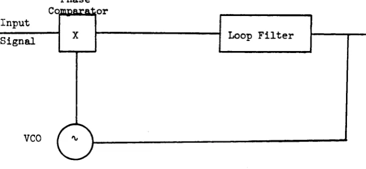
A phaselock loop (U) contains three basic components (Figure 2.1);

a phase conq)arator, a low pass filter and a voltage-controlled

oscillator (VCO).

Input

Phase Comparator

Signal Loop Filter

VCO

Ô

Fig. 2.1 Basic Phaselock Loop

The phase comparator compares the phase of a periodic input signal

against the phase of the VCO. When the phase differs from 90° (a

condition which will exist when the input signal tries to change

frequency) the phase comparator will immediately sense the phase

difference and provide a dc error output voltage proportional to the

cosine of the phase difference. The phase comparator does not permit

a steady state frequency error to be developed between the VCO and the

input signal. This is due to the integration of the frequency changes

by the phase comparator which produces the error voltage proportional to

phase difference.

This error voltage is applied to a low pass filter where high

frequency components are suppressed. This filter also determines the

dynamic performance of the loop.

The output of the loop filter is applied to the VCO to control its

frequency about the center frequency. The center frequency of the

klystron oscillator is determined by a mechanical tuner and by the

reflector voltage. The error voltage output from the filter is summed

with the reflector voltage from the klystron power supply and fed to the

reflector of the klystron oscillator to control the output frequency of

the klystron.

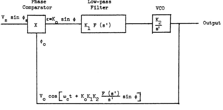
An analytic block diagram showing the operations of a phaselock

loop is illustrated in Figure 2.2 (5).

Phase Comparator

Low-pass

Filter VCO

Output

sin

2.2 Analysis of Loop Equations

Consider the loop shown in Figure 2.2. The input signal has a

phase of *g(t), and the VCO output has a phase (t). It is assumed

that the loop is locked and the phase comparator is a perfect multiplier.

Suppose that the input signal is

(t) ■ Vg sin (*g)

and the VCO waveform** is

Vq (t) - V^ cos (+o)

Output of the phase comparator (neglecting double frequency terms that

will be removed by the loop filter) is:

V o \ CO. [90» - (*, - *,)]

or

where is a constant of proportionality of phase comparator output,

i.e., the output of the phase comparator is

Using the notation of Figure 2.2

K = K V V

o m s o

Therefore,

e = sin (*g

-* sin * (2-2 )

**Note that v^ and v^ are really 90° out of phase with one another.

The input has been written as sine and the VCO output is a cosine. The two phases and are referred to these quadrature references.

or E = K_ sin (*_ (t) - w_ t - K_K,K„ F(s') sin 4») (2-3)

0 S C O X & 0

8

Comparison of equations (2-2) and (2-3) yields

* = *g (t) - w^t - KgK^Kg F(s) sin *

differentiating with respect to time and defining K ■ K^K^K^, the overall

loop gain, gives

$ + K F(s) sin <t> “ 4>g - Ug (2-4)

The transfer function for the loop filter in the present system is

F (s') = 1 + TS*

1 + a TS*

where t is a time constant and a is a factor of proportionality greater

than one.

Equation (2-4) becomes

$ (l + a TS*) + K (l + t s) sin <|i = ({i^ - w^) (l + a t s)

or

<}) + + lia. sin 4i + K sin <p ^ (p + (* - w ) 1^ (2-5)

OT a OT ® ® ° aT

Since it was assumed that the loop was locked the linear approximation

sin 4» 4" can be made. This gives

+ / K + 1 ^ ^ — (^g + (^g — ) 1 (2—6)

\a OT/ OT OT

The left hand side of equation (2-6) can be compared to the second order

•# * 2 $ + 2 c w t + w 6

n n

Equating appropriate terms gives

u - ^ (2-7)

and

w / Kt + A ~ ^ J

(2-8)

substituting into equation (2-5) gives

y + ^1 + T cos *) * + sin 4> * 4» + (♦ - w )

(2-° \iT / s 8 c n 9)

The input frequency $g is composed of the initial frequency plus the step

change of frequency

^s * (2-10a)

where u (t) = 1 t v 0

« 0 t < 0

differentiating (2-lOa) with respect to time gives

4> * A(i) du (t) (2-lOb)

® dt

On substitution of equations (2-lOa and b) into equation (2-9) one

obtains

4» + 10^ (1 + T cos (f) 4* ♦ sin 4* * du du (t) + u^ u (t)

" K " dt ^

or upon integrating with respect to time.

10

sin * dt .

• r 2

"1

3

4» ■ Auj u(t) + w t j - o ) 4> - w T I cos ^ 4> dt - w n

1? 4 ” J

Integrating the third term on the R.H.S. we obtain

* 1 2 T 2 2 2 ^

6#,|u(t) + u^ t - T sin * - rsin 4» dt (2-11)

Î T k“ 4

where integration has eliminated the "infinite discontinuity" ^ (t) . dt

Equation (2-ll) is programmed on a digital computer using analogue

simulation and the resulting phase plane and time trajectories for an

11

2,2.1 Linear Analysis of Transient Phase Error

The output of the phase comparator is given as (equation 2-2)

c » sin (*g - *^) (2-12)

now ■ Kg Vg (2-13)

where Vg is the output of the filter.

Transposing to the frequency domain gives

K, V (s) (2-14)

♦c <') - - 4 ^

Referring to Figure 2.2 the output of the filter is given as

Vg (s) = F (s) E (s)

» (s) - (s)j F (s) (2-15)

where the linear approximation sin * + * for ♦ << £ is included. 2

Substituting equation (2-15) into (2-l4) and performing the required

algebra yields

i (s) K K F (s)

O O c

and

à (s) " s + K K- F (s)

S O c

4^ (s) - (s) 4 (s) 8 (2-16)

*g (s) “ ♦g (s) “ 8 + K^Kg F (s)

where * is the phase error.

For a step change of frequency of magnitude Aw

<P (s) Aw (2-17)

8 ■

12

Substituting equation (2-17) into (2-l6 ) and applying equations (2-7)

and (2-8 ) gives

4> (s)

Aw (s + )

(s + 2Ç W s + w 2 )

n n

Transforming back into the time domain yields

4 (t) = Aw 1 . 1 r v "n + n

_ K2 " K

-ll/2

e-c w^t

. sin ( \J~1 - 'w^t + Y T[

(2-16)

where

Y =^tan"^ ^

n

T"he steady state value of phase error is

. Aw

♦ss " r

The time for the transient phase error to decay to zero varies with

the values of ç and w^, the loop parameters. Once the loop is chosen

the decay time depends only on the magnitude of the frequency step Aw.

Therefore to obtain small lock in times a compromise has to be made in

the size of the frequency step. This would handicap most communication

systems dependent on step frequency transitions.

2.3 State Variable Analysis of Loop

13

of the output of the signal source following a step change in frequency.

The second method, frequency control, consists of controlling only the

frequency of the signal source. The emphasis is centered on the latter

method of control in this paper. The two methods of control are

illustrated in Figures (2.3a and h)++

Aw

Frequency Control

-

o

Phase Control

Phase

Shifter _______ To

Phaselock Loop

(a)

Aw _To

Loop

u

(h)

Fig. 2.3 Signal Source (a) Physical System (h) Voltage Analogue

++

Up, (t). Aw, Up (t) and v (o) may he considered as voltages which are

summed and fed into a VCO. The dimension of the gain constant for the VCO is me .

volt

14

During phase control, the oscillator frequency is stepped hy an

amount Aw at t - o, the oscillator output is phase shifted by an amount

Up(t) for t ^ o, and Uy(t) ■ o. During frequency control, the

oscillator frequency is stepped by an amount Aw at t * o, and is

additionally changed by Up,(t) for t ^ o. In this case u^(t) ■ o.

For frequency control, the frequency of the oscillator is

Ab) + Up(t), t > o

For phase control, the phase of the phase shifter output is

V

= u^(t) + ((Aw + V (o) ) dt

= u^(t) + (Aw + V (o) ) t, t > o .

The initial frequency of the input signal v (o) is made equal to the

VCO center frequency w^ in order to eliminate tuning error from the

analysis.

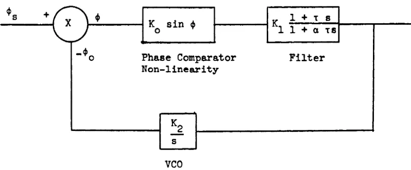
A block diagram showing the input phase and the phase comparator

non-linearity is illustrated in Figure 2.U.

Phase Comparator Non-linearity

Filter

15

The loop shown in Figure 2.U is reconstructed with the signal source

included as shown in Figure 2.5. This representation is known as the

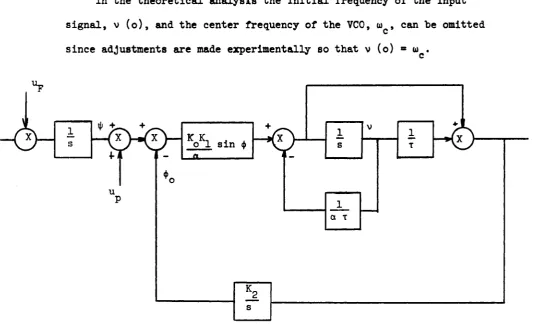
state veuriable diagram (6), and the output of each integrator is called

a state variable. The state variables chosen are i}», v and as

shown in Figure 2.5. The loop filter has been represented in terms of

summers, amplifiers euid integrators using the method of direct

programming (6).

In the theoretical analysts the initial frequency of the input

signal, V (o), and the center frequency of the VCO, w^, can be omitted

since adjustments are made experimentally so that v (o) = w^.

1 V 1

s T

o 1 sin d)

Fig. 2.5 State Variable Diagram of Loop

16

2.3.1. Optimum Frequency Control

Writing the differential equations of the loop by inspection of

Figure 2.5 gives

* = Aw + Up (2-19a)

K K,

*o = ^2 T + sin (2-19b)

. K K

V = — — sin (* - * ) - — - (2-19c)

a O QT

These equations are the state differential equations for the loop.

Initially * (o) = o .

The problem is to find ty, such that <}i (t^) = o and the frequency

error at the terminal time, t^, is zero, t^ being a minimum.

In order to simplify equation (2-12) the definition

^ (2-20a)

Eind

K

Xg = Aw - [^1 - V (2-20b)

is made, where x^ and Xg are phase and frequency error respectively.

Substituting equations (2-20) into (2-19) and utilizing the servo

terminology of equations (2-7) and (2-8) yields

x^ = - w^^ T sin x^ + Xg + u^, (2-21a)

^ 2 ^ 2

Xg = - w ^ ^ sin X., - -s— x_ +

zp—

17

with initial and final conditions

(o) = o , Xg (o)=Au) and x^ (t^) * Xg (t^) = o .

Pontryagin's maximum principle, as outlined in Appendix I, is now

*

applied to equations (2-21) in order to find the control, u^ , which

minimizes t^ .

A new state variable

Xg = ^ dt * t (2-22)

is defined such that Xg = 1, and Xg (o) = o .

The Pontryagin function P is given by

P = x^ (tj) + Wg Xg (tj) + Xg (2-23)

The optimum design problem now reduces to the determination of the

admissable control, Up ^ |Up| so that the Pontryagin function is

minimized.

The hamiltonian for the system is

^ g-1 sin Xj a

2 w

+ ( Aw - Xp))+ p., (2-2U)

where the costate (or adjoint) vectors p^, Pg and Pg are related by the

canonical equations

18

2

• 3H

P2 = - Pi + — P2 (2-25b)

P3 = - ■ O (2-25c)

which describe the adjoint system, subject to the boundary conditions

Pi (tj) = and Pg (t^,) = y^. Since pg (t) « o and Pg (t^) = -1,

Pg (t) = -1.

Examination of the hamiltonian H reveals that it is a maximum with

respect to Up if

Up* = |Up| sgn p^ (2-26)

In order to obtain u*p with respect to time, equations (2-21) and

(2-25) are solved in conjunction with (2-26).

The above equations are readily adaptable to an analogue computer.

A trial and error method of finding the initial conditions of the costate

vectors p^ and pg must be used. The initial conditions p^ (o) and

p_ (o) must be chosen so that the final conditions x. (t.) ■ x (t ) = o

d i 2

are satisfied. The final conditions on the costate vectors p^ (t^) and

Pg (t^) are open since in Pontryagin's function the final conditions on

x^ and Xg are zero.

2 .3.2 Linear Analysis of Frequency Control

Allowing Aw = 0.5 w^ and |u| = w^ it may be assumed with small

error that

sin x^ « x^

19

equations (2-21) are normalized. With these assumptions equations (2-21)

become

(2-27a)

with (o) ■ o, and Xg (o) ■ “ • n

In matrix notation this is

(2-27b)

where

and

; _{X = *1} ; u =

*2 _• Aw_m

g-1 “n

g "K

B = 1 “n

o Aw

(2-28)

“n

Using the state transition method (7) of solution and solving by means of

Laplace transforms yields

^ (s ^ L ^ (s) X (o) + 8 (s) B u (s)J

\-l X (t) = L

where 0 (s) = (si - A)'

and I is the identity matrix. The solutions to equations (2-27) in terms

20

of normalized time, w^t are

(t) ■ Aw

. sln(J 1 - ê " V . ^l) + l'^

where

and

^ (s)

2 ’

s + 2c 8 + 1

(2-29a)

1 1

“ «f

(l - a )*- G 4|l - ç 2 ' + y^)

1 - Ç

+ L-1

a - 1

***n g (s)

8 + 2Ç 8 + 1

(2-29b)

Yg = tan-1

These equations for phase and frequency error illustrate that when

the loop parameters have been fixed, and a specified step in frequency

introduced into the input that the decay times of x^(t) and Xg(t) can

still be controlled by applying a control Up. Since |up| = * U, it is

observed from equations (2-29) that Up can be switched in a manner, so as

to have a direct effect on the values of x^ and Xg.

Comparison of equation (2-29a) with (2-l8) demonstrates that applying

21

2.3.3 Optimum Phase Control

Setting Up » o and writing the differential equations of the state

variable diagram illustrated in Fugure 2.5 yields

i = Aw (2-30a)

K K

= Kg Q " sin + Up)j (2-30b)

K K

V = — — sin - * + u \ - —

a ^o pJ oT

Substituting State Variables and Xg from equation (2-20) gives

x^ = -“n^T gin( x^ + u ) + Xg (2-31a)

X- = - % 2 “ - — sin (X- + u ) - % 2 % + "^n^ Aw (2-31b)

2 a V 1 p; _ 2 —

The initial and final conditions are the same as before:

x^ (o) = o , Xg (o) = Aw , x^ (t^) = Xg (tp) = o

The problem is to determine u^ such that t^ is minimized. Again the

Pontryagin function is

with

P = (t^) + Wg Xg (t^) + Xg (t^) (2-32)

Xg = ^ dt = t . (2-33)

The hamiltonian, as shown in Appendix I is

22

H - [Pi + Pj u.^2 (1 - i) ]sln (Xj^ . u^) * _Xg

0) 2

+ Pg jj A(Ü + Pg (2-34)

The adjoint equations are then

Pi = " p i “n. " * P2 “n < p - a ''‘l * “p> '=-35»>

0)2

Pg = - i;- = -Pi + K^- P2 (2-35b)

Pg = o (2-35c)

with the final conditions on the costate vectors p^ and P g open as in

frequency control. The hamiltonian, H, is maximized with respect to u^ if

sin (x^ + Up) = - sgn (p^ wf ? + pg ( 1 - ^ ))

or

7T 2 2 1

U» » - x^ - — sgn (p^ T + P g (1 - — )) (2-36)

With this value of u^, the system state variable differential

equations (2-3l) and the adjoint equations (2-35) reduce to

X, = + uf T s g n (p, wf T + p „ o)f (l - % )) + X g (2-37a)

i n i n c n a d

* 2 g-1 f 2 2 . 1\% w 2

23

= o or p^ = p^ (o) (2-37c)

w 2

Pg = (°) + K— Pp (2-37d)

Solving equation (2-37d) gives

w^2 .

Kp Kp (o) =—

P2 (t) - ^Tg - Pg (o) - --- e (2-38)

n n

where p^ (o) and Pg (o), the costate vector initial conditions, are

chosen by a trial and error method to give the optimum control u* .

An interesting feature to note in the above analysis is that the

introduction of phase control has eliminated the sine non-linearity in

the State Variables and Xg . The above system may now be analyzed by

ordinary linear methods without incurring the restrictions due to the

use of a linear approximation.

2.3.4 Analysis of Optimum Phase Control

Rewriting equations (2-37a) and (2-37b) in terms of normalized

time, w^t, yields

x^ = Xg + w^T sgn q (2-39a)

Xg = Xg + sgn q + ^ (2-39b)

where

q - V * Pg

which in matrix notation becomes

24 -w n K 0-1 a

1

X * Ax + Bu

Solution by state transition method (8) gives

X = G (t) x^ + ^ 8(t-f) Bu dT

where

0 sgn q

; u =

All) Au)

(I) n

0 (t) = L~^ (sI-A) ^ , the transition matrix

Expansion of equation (2-4l)yields

x^(t) = 8g + d^ sgn q + dg Au) n

(2-4l)

(2-42a)

%2(t) = *4 + *2 *60 q + % Aü) (2-42b)

where

= J Ç s i „ _ p t • 8^ = COS I — t

nr\

f '

di = U - l  ( % ) ' sln f|]n t

25

K

'"(F'

d. ^ ( l - 008 j ^ t j .

with

sin ^ w

r g-1 _2_ I 5 _

h ‘ tan-1 ^

f-n

As in frequency control, sgn q, has an effect on the phase and

frequency transients.

Phase trajectories of equation (2-42) can be plotted for sgn q = 1

Euid sgn q = -1. The optimum trajectory may be determined from these

trajectories.

17715

M ÏER SITY OF MOSQR UBRARl

CHAPTER III

ABALOGUE COMPUTER SIMULATION

3.1 Procedure

The differential equations for phase and frequency error derived in

Chapter II, autonomous for t > o allow an accurate solution to be obtained

by analogue methods. The state variable system is simulated in

conjunction with the adjoint system which supplies the control vector.

The trajectories of the system are obtained by Pactolus Digital

Analogue Simulator Program (9). The program is incorporated into an

IBM 1620 MK II digital computer and the trajectories are plotted by a

CALCOMP on-line plotter. Pactolus allows direct control of the costate

initial conditions via an on-line typewriter.

The equations are simulated in terms of normalized time, w^t, in

order to avoid exceeding the numerical bounds on the computer.

3.2 Locking Without External Control

Rewriting equation (2-11) in terms of normalized time yields

^ ^ ^ ^ ^ - X 0)^ sin ♦ - ^sin ^ dt (3-1)

An analogue block diagram of equation (3-1) which consists of

integrators, summers, amplifiers, inverters and other blocks which are

elements of the Pactolus program is shown in Figure 3.1. The parameter

values for the loop are given in Appendix II. The related Pactolus program

for Figure 3.1 is given in Appendix III.

27

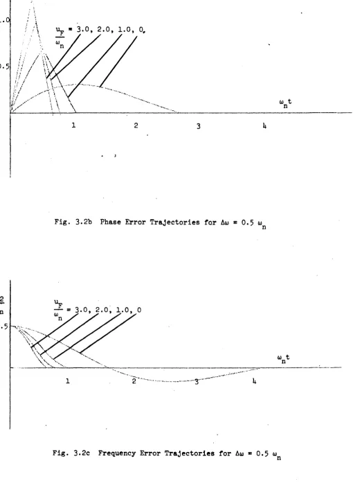
Figure 3.2a shows the phase plane trajectories® for step frequency

inputs of Aw = 0.5 . Figure 3.2b and c illustrate a plot of phase

and frequency error versus time.respectively. Figures 3.3 show the

above curves for Aw * w n

The phase plots of the uncontrolled systems (Figures 3.2a and 3.3a)

start at a frequency error of Aw at time t ■ o and spiral to a point of

zero frequency error and positive phase error. This point is the steady

state phase error of the system which is 0.032 (radians) for Aw = 0.5 w^

and 0.064 (radians) for Aw * w n

When the size of the step frequency input was doubled from 0.5 w^

to w^ the time for the frequency transients to decay from their maximum

values to within 5% of their steady state values increased from 8.15 to

8.50 units of normalized time.

3.3 Locking with Frequency Control

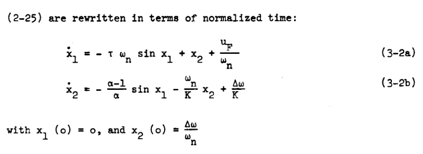
For convenience, equations (2-21) along with the adjoint equations

(2-25) are rewritten in terms of normalized time:

X, = - T w sin X, + X- + (3-2a)

1 n 1 2 w

n

with x^ (o) = o, and Xg (o) = ^ n

°Phase plane trajectories are a plot of frequency error versus phase error with time a parameter along the path length.

28

Pi = cos jp2 ^ Pp ^ (3-2c)

w

Pg “ “Pi i f P2 (3-2d)

These equations are simulated for Pactolus programming by the

analogue block diagram of Figure 3.4. The corresponding program is given

in Appendix III.

Figure 3.2a shows the phase trajectories for a step frequency input

of Aw = 0.5 and control vector amplitudes of Up« w^, 2w^ and 3w^ .

Figure 3.2b and c show the corresponding plots for phase and

frequency error respectively, versus time.

Figure 3.3a shows the phase trajectories for a step frequency

input of Aw = w with control vector amplitudes of 0.5 w , w_ and

^ n F n n

1.5

Figure 3.3b and c show the corresponding time domain plots for phase

and frequency error respectively. Superimposed on the above curves are

plots of uncontrolled trajectories for comparison.

Figure 3.5 illustrates the shape of the control vy* . The

numerical values for the parameters in Figure 3.5 are given in Table 3.1.

Table 3.1 gives the resulting switching times t^, and t^. It is observed

that as the magnitude of the control is increased, the decay times of

2Q

% "n t. "n tf

0.0 8.150

1.0 0.650 1.330

2.0 0.510 _0.995

3.0 0.1*50 0.850

(a)

% “n \ “n tf

0.0 —— 8.500

0.5 0.790 2 .UOO

1.0 0.800 1.850

1.5 0.750 1.620

(t)

Table 3.1 Transient Decay Times, (a) ^

u 0.5 — - 1.0

It was found that for Aw = w^ the loop could not achieve lock for

Up > 2w^ . This occurs because the phase error has surpassed the lock

range of the loop.

The portion of the phase plane curve prior to the first switch

occurring at time t^ is found to be identical for all combinations

of costate initial conditions tried with Aw and U.^ remaining constant.

The costate initial conditions determine only the time of the first

30

switch tg. In addition the portion of the curves following the switching

time tg are nearly linear translations of the same curve.

This allows the optimal initial conditions to he found with relative

ease; in fact five trials of different initial conditions prove to be

sufficient to find the optimal control.

Table 3.1 illustrates the great improvements possible in minimizing

31

CO •H 00

LTV

\o

I

"O 0)

0 k

1

ê 4-,

o

Ad

0

W

1

on

Û •H

32

(radians)

"F j \

z- - ° — \

1.0

(radians) .

1

.

0

.

Fig. 3.2b Phase Error Trajectories for Aw = 0.5 w

X

2

w n

0.5

Fig. 3.2c Frequency Error Trajectories for Aw » 0.5 w

34

(radians)

m

1.0

(radians)

1.0

35

«

l.C

Fig. 3 .3b Phase Error Trajectories for Aw = w_

2

n

1.0

Fig. 3.3c Frequency Error Trajectories for Aw = w

36

OJ

m

.

CO

VÛ

CM

rH

cn

o\

o

& o

'Ü (U

0 k

1

o «M

o

u 0 iH PQ (U

1

cn

%

•H

37

Fig. 3.5 Control Vector Waveform

CHAPTER IV

SYSTEM DESIGN

U .1 Experimental Setup

The phaselock loop utilized in the experiment is incorporàted in a

Dymec Oscillator Synchronizer Model DY-2650A. The DY-265OA is used to

stabilize a voltage controlled oscillator in the frequency range of

1 to 12.U Gc. The VCO used is a Varian X-13 reflex klystron which

operates in the x band (8.2 - 12.h Gc). A small sample of the klystron's

signal is mixed with a harmonic of the signal from a

temperature-stabilized crystal r-f reference oscillator, either internal or external,

to produce a 30 me i-f signal. (See Figure 4.1). This i-f signal is

then phase compared to an i-f reference signal. When lock is obtained

any attempts by the klystron to shift frequency will produce a phase

error and a phase comparator output voltage which is applied in series

with the reflector supply to stop the frequency shift.

The approach taken to obtain experimental results is to first

lock the klystron to a known frequency, ensuring that the phase error

is zero. The output of the phase comparator is monitored on eui

oscilliscope. The step change in frequency plus the control are fed

to the reflector via the external modulation terminals on the klystron

power supply. These voltages are fed repetitively so that a visible

trace can be observed on the oscilliscope. The repetition rate is set

to give the loop time to relock to its initial state.

39

X

=! = >-<o uo c: °

go u < c o < Ô % Ü

3

z

o

z

g

o

I

40

§

§ 0 ■p k a;

1

+3 CQ

V 0) A C

CO b

0) §* o

Ü o «

&

t

CO

CÔ

I

I

C\j

41

h.2 Method of Introducing Frequency Step and Control Function Input

In the theoretical analysis the frequency control is summed with

the step frequency change and applied to the phase comparator. It was

assumed that there is zero tuning error, i.e. that a condition is set

up so that the input initial frequency is equal to the VCO centre

frequency. In a practical system this requires a very stable rf

generator which could be frequency modulated with a pulse and have an

output which could furnish the required amplitude of at lease one volt

to the VHF terminal of the harmonic mixer.

The rf reference circuit which consists of a crystal oscillator,

provides the stability necessary to give zero tuning error, but it is

not possible to frequency modulate the rf reference circuit. This

difficulty is avoided by applying the step change in frequency at a

portion of the loop other than the input.

Figure U.3a illustrates a simple negative feedback control loop

(a)

(b)

Fig. 4.3 Negative Feedback Loop

'H

it

42

The output of the summer is given as

6 (s) = r (s) - h (s) ■ - (-r (s) + h (s) ) (k-l)

now h (s) is given as c (s) G (s). Therefore equation (U-l) becomes

6 (s) = - (-r (s) g + c (s) G (s) )

or

6 (s) = - (c (s) - G (s) (U-2)

In other words, the output of the summer will not change if the

input, r, is summed with the output, c, in the manner shown in Figure U.3b.

Applying this technique to Figure 2.5 results in Figure U.1+, where the

filter is lumped into one block.

o ~ .

43

Au) and u* will have their amplitudes changed by a factor of 1_ .

It is now possible to add 1_ (Aw + u_,) in series with the reflector

supply. This gives the required conditions of experimental analysis.

k.3 Design of Frequency Control Function

The control function of Figure 3.5 can be broken down into the

addition of two pulses, one positive and one negative, of equal amplitude.

The negative pulse is delayed by t^ seconds before being summed with

%

the positive pulse. The positive pulse is obtained from an

emitter-coupled monostable multivibrator whose pulse duration is made equal to

t . A second multivibrator furnishes a pulse of duration t_ - t to

s ^ f s

%

an inverter circuit. This second multivibrator is triggered by a

delayed trigger. This delay is equal to t^. The step change of

frequency Aw is obtained from a third monostable multivibrator with a

long duration pulse and a magnitude of Aw. All three pulse are

algebraically summed by a high gain dc amplifier. The output of the

high gain amplifier is fed in series with the reflector power supply.

The delay of t seconds is obtained by passing a pulse through the

required number of feet of transmission line. The above circuit

implementation is summarized in the block diagram of Figure U.5.

üfflïEaSITY OF WfflBSQR lIBRMï

44

i

Trigger

MV 1

MV 2

Delay

MV 3

Long Durât ion

Pulse

CHAPTER V

EXPERIMENTAL RESULTS

5.1 Response of Loop to Step Frequency Changes

A step change in frequency was obtained by turning off the first

and second multivibrators, MVl and MV2 in Figure U.5. An exact replica

of a step change can not be obtained since there is capacitance in the

leads leading from the summer to the reflector, and approximately 20 pf

of capacitance shunting the reflector to ground. This causes a large

increase in rise time of the desired step change.

Table 5*1 gives the values of phase error settling times obtained

by analogue and experimental methods for Aw = 0.5 w and w . The

n n

experimental results are accurate to within 20%. The reason for this is

poor definition of waveforms available on the oscilloscope (see Figures 5-1)■

The thickness of the waveform is due to 30 Me leaking through the phase

comparator.

Although there is no direct method of measuring the decay time of the

frequency error, or, the exact amount of frequency change by the klystron

oscillator, an indication of frequency change is noticed when the repetitive

pulse returns to its initial condition by a disturbance of the phase error.

This disturbance in phase error approaches that due to a quasi-static

change because of the long decay time of the switch to the stable state.

5.2 Controlled Step Frequency Changes

When the step change plus control (Figure 5.2a) is applied to the

45

46

reflector of the klystron, the waveform visible at the reflector

(Figure 5.2b) is distorted and attenuated. This distortion due to

capacitance of leads and reflector to ground capacitance can be removed

by using a compensated probe to apply the signal from the summer amplifier

to reflector. Since the compensated probes have an attenuation factor of

10:1, the amplitude of the pulses at the summer have to be magnified by a

factor of 10 which causes saturation of the summer amplifier.

Another method of applying the control signals to the reflector is by

an active probe using an emitter or cathode follower configuration. The

emitter follower is not applicable since it is required to be able to

follow a signal which switches between * 20 volts.

A cathode follower circuit was constructed using a pentode tube.

This circuit can not follow the speed of switching of the control signal

which has a rise time of 20 nanoseconds.

When the signal is applied using the cathode follower circuit

the waveform which appears at the reflector is shown in Figure 5.3a. The

output of the phase comparator is not an optimum response. This is

expected since the control signal is not the optimum control designed.

Application of the distorted control signal does indicate that the

phase error response is changed by a significant amount (Figure 5.3b)

from a simple frequency step. The phase error response does not approach

the response calculated by analogue methods since the control

47

n

1.0

*^n

Experimental ^ 2 5 ys ^ 27 ys

Results

Computer 21.5 ys 22.U ys

Results

Table 5.1 Experimental Decay Time for Step Change in Frequency

48

(a)

(b)

Fig. 5-1 Phase Transient Trajectories (a) Aw = 0.5 w

49

(a)

(b)

Fig. 5*2 Control Function Input (a) Control Generated

(b) Control After Applying to Reflector

(Time scale of (b) is tripled)

50

(a)

(b)

Fig. 5.3 Application of Distorted Control Function (a) Pulse Applied to Reflector

CHAPTER VI

DISCUSSION OF RESULTS

6.1 Theoretical

Application of the maximum principle to a second order phaselock

loop has produced an extremal frequency control which is locally optimal

for a specified magnitude of control vector U_. The theoretical

derivation was relatively straightforward.

Optimum phase control has removed the sine non-linearity in the

state variable equations allowing a linear analysis approach to the

problem. Although phase control is less difficult to handle theoretically,

it would be an experimental problem of considerable magnitude. The

construction of a phase control vector being the main problem, for

although it would switch in the same manner as u* , its amplitude between

switching depends on x^.

The results from analogue simulation illustrate that a considerable

improvement in minimizing transient decay times is obtained. (See Table 3.1)

The optimum control vectors are u* = 3 sgn p^ for Aw = 0.5 w^

and XI* = 1.5 w sgn p. for Aw = w . This leads one to the obvious

conclusion that the optimal control is obtained by increasing the magnitude

Up, to maximum limits without the loop going out of lock.

Solution of the boundary value problem to obtain p^(t) is accomplished

by a trial and error method of searching for the costate initieü. conditions

which satisfy the final conditions on x^ and Xg. The trial and error

method of search is made easier if an on-line plot of phase trajectories is

available to allow visualization of the effect of changing p^(o) and Pg(o)

51

52

has on the switching times of the control vector.

6.2 Exper iment al

The difficulty encountered in the acquisition of experimental results

is the "state of the art" problem of transferring a fast rise pulse from

point a to b with minimum distortion at b. The most logical approach to

this problem is construction of an active probe which presents a very

high impedence to the output of the summer amplifier and a low output

impedence which is capable of driving the klystron reflector.

The results that were obtained demonstrate the feasibility of this

type of control if experimental problems can be overcome. These problems

are construction of the control cycle waveform, introducing the control,

and an accurate method of measuring the results of application of a

control signal.

By applying the control of the input of the VCO as shown in Figure U.3b

a degree of adaptability is obtained. Since the adjoint system which

generates the control vector depends only on the cosine of the phase error

and costate initial conditions, a black box could be constructed with the

input being phase error and the output being the control signal which has

a predetermined maximum amplitude. The input signal could then change

frequency and the control would change its switching time appropriately

to minimize the settling time of the transients.

6.3 Conclusions

This paper has investigated the method of optimal control using the

53

it has been shown that a control vector can be constructed and that it

does effect the performance criteria.

The theoretical derivation of optimality does not present any major

difficulties aside from handling cumbersome equations. The control vector

obtained is optimal. This is shown by the analogue computational results.

An application of this work would be to minimize the time required to

change the frequency of the transmitter by an amount greater than the lock

range of the loop. This could be done by changing the frequency of the

transmitter in discrete steps,each step being the maximum lock-in range

for a step change in frequency. This would produce a staircase transition

from one frequency level to the next.

A particular extension of this work would be to find the relation

of the magnitude of the step change in frequency and optimal control

vector to the value of the costate initial conditions. Such information

would lay the path for a completely adaptable receiver for frequency

transitions of the input. Such a receiver would be applicable to following

a frequency pulse modulated signal.

In general it is very difficult to design an optimal system in

accordance with the mathematical theory. The reason for this is that the

design of a system involves many engineering Judgements regarding such

facts as simplicity, reliability, cost, etc., which cannot be neatly

expressed in a mathematical statement. Although the exact optimal system

is seldom constructed, knowledge of the truly optimal system will provide

the engineer with a well defined starting point and a yardstick for ultimate

performance.

A peurticular advantage of the necessary conditions for optimality

54

provided by the maximum principle is that, vith very little analytical

effort, one can often deduce certain properties of the optimal control and

of the structure of the optimal control system, without ever going through

APPENDIX I

FUNDAMENTALS OF PONTRYAGIN'S MAXIMUM PRINCIPLE

Consider a nth-order control process characrerized by

X = f (x, u, t)

where x is the n x 1 state vector and u is the input n x 1 control

vector.

At each moment the control signals u^ must satisfy the inequality

constraint g (u) ^ o which reflects the restriction imposed upon the

control system. The control vectors which satisfy the constraint

condition are referred to as admissable control vectors.

The above process is optimized by forming a criterion of performance

for the above system and maximizing or minimizing this criterion by an

external control inaccordance with given constraints.

This criterion of performance is measured in terms of some

functional

n

P = I b. X. (t_) i=l

or P = ]b/ :K (t^)

where b is a n x 1 column vector. P is called Pontryagin's function.

When the final state of the process is constrained by

\ (^f)^ “ ° k = 3,^. • VÎ V £ n

Pontryagin's function takes the form

P = b X (t^) + U R Qc (t^)J

where £ is the vector lagrange multiplier.

55

56

The maximum principle states that if the control vector u is

optimum, i.e., if it extremizes the Pontryagin function P, then the

hamiltonian for the system is extremized in the opposite direction with

respect to u over the control interval.

The hamiltonian is defined as

H (x, 2 , u,t ) = Z P. f,

j - 1

(A 1-1)

where p analagous to the canonical momenta in classical mechanics, will

be defined later. The f^'s are the system’s state variable equations.

The above statement implies that maximum H will give minimum P and

vice-versa. Thus a necessary condition for the control vector u to

optimize the Pontryagin function is the fulfillment of the maximum

condition for H.

To apply the maximum principle in the solution of optimum-control

problems, the design procedure is initiated with the maximization of

hamiltonian H with respect to the control vector u.

This results in an optimum control vector u* as a function of the

momentum vector £. In order to find u* as a function of x or t ,

equations providing the relationships between u and £ must be

established.

We first define the momentum vector £ as the solution to the

differential equation

n

p. = - Z p 3f. i = 1,2, ....n. (a 1-2)

V

57

Pi (tj) " - (A l-3b)

where b^ is a known constant specified by the designer in the Pontryagin

function P and

* fj (x u t) (A 1-U)

Differentiating equation (A l-l) with respect to yields

3H = fj ( X u t ) (A 1-5)

Differentiating equation (A l-l) with respect to gives

n

3H = I P 3f (A 1-6)

Making use of these two equations reduces equations (A 1-2) and (A 1-U) to

the Hamilton canonical form

X, = 3H (A l-7a)

‘ â T

p. - - 3H_ (A 1-Tb)

^ 3x,

subject to the boundary conditions on (t^) and p^ (t^).

The minimum time problem may be stated as the determination of an

admissable control vector u so that the process is taken frcxn a

specified initial state x to a desired final state ^ in the shortest

— o — T

possible time. The control signals being subject to the constraint

H

where U is the largest magnitude available for u.

58

By introducing a new co-ordinate

X . (t) - \dt " t - t

n+i 1 o

to

the optimum control problem becomes a minimization of the new co-ordinate

which is our criterion of performance. The differential equations of

the system are now

^1 ■ q &

^

subject to the initial conditions x (t ) * x

— o o

The Pontryagin function will be

(tf) * 5 . 1 "j *3

V i ■ ^ •

This gives (see equation A 1-3)

Pi (tfj = o ,

*0+1 •

59

Maximizing the hamiltonian with respect to u euid applying equation

(A 1-Th) to (A 1-8) furnishes the proper relations between u and t.