Which Ring Based Somewhat Homomorphic Encryption Scheme is Best?

Which Ring Based Somewhat Homomorphic

Encryption Scheme is Best?

Ana Costache and Nigel P. Smart

Dept. Computer Science, University of Bristol,

Bristol, UK.

[email protected],[email protected]

Abstract. The purpose of this paper is to compare side-by-side the NTRU and BGV schemes in their non-scale invariant (messages in the lower bits), and their scale invariant (message in the upper bits) forms. The scale invariant versions are often called the YASHE and FV schemes. As an additional optimization, we also investigate the ffect of modulus reduction on the scale-invariant schemes. We compare the schemes using the “average case” noise analysis presented by Gentry et al. In addition we unify notation and techniques so as to show commonalities between the schemes. We find that the BGV scheme appears to be more efficient for large plaintext moduli, whilst YASHE seems more efficient for small plaintext moduli (although the benefit is not as great as one would have expected).

1

Introduction

Some of the more spectacular advances in implementation improvements for Somewhat Homomorphic Encryption (SHE) schemes have come in the context of the ring based schemes such as BGV [3]. The main improvements here have come through the use of SIMD techniques (first introduced in the context of Gentry’s original scheme [7] by Smart and Vercauteren [17], but then extended to the Ring-LWE based schemes by Gentry et al [3]). SIMD techniques in the ring setting allow for a small overall asymptotic overhead in using SHE schemes [8] by exploiting the Galois group to move data between slots. The Galois group can also be used to perform cheap exponentiation via the Frobenius endomorphism [9]. Other improvements in the ring based setting have come from the use of modulus switching to a larger modulus, so as to perform key switching [9], the use of scale invariant versions [6, 1], and the use of NTRU to enable key homomorphic schemes [14].

The scale invariant schemes, originally introduced in [2], are particularly interest-ing, they place the message space in the “upper bits” of the decryption equation, as opposed to the lower bits. This enables a more effective noise control mechanism to be employed which does not on the face of it require modulus switching to keep the noise within bounds. However, the downside is that they require a more complex rounding operation to be performed in the multiplication procedure.

scheme [5, 14], and its scale invariant version YASHE [1], rarely, if at all, make men-tion of the use of SIMD techniques. Papers working on scale invariant systems [6, 1] usually focus on plaintext moduli of two, and discount larger moduli. But many appli-cations, e.g. usage in the SPDZ [4] MPC system, require the use of large moduli.

We have therefore conducted a systematic study of the main ring-based SHE schemes with a view to producing a fair comparison over a range of possible application spaces, from low characteristic plaintext spaces through to large characteristic ones, from low depth circuits through to high depth ones. The schemes we have studied are BGV, whose details can be found in [3, 8, 9], and its scale-invariant version [6] (called FV in what follows), the basic NTRU scheme [5, 14], and its scale-invariant version YASHE [1]. A previous study [12] only compared FV and YASHE, restricted to small plaintext spaces (in particular characteristic two), and did not consider the various variants in relation to key switching and modulus switching which we consider. Our results are broadly in line with [12] (where we have a direct comparison) for YASHE, but our estimates for FV appear slightly better.

On the face of it one expects that YASHE should be the most efficient, since it is scale invariant (which often leads to smaller parameters) and a ciphertext consists of only a single ring element, as opposed to two for the BGV style schemes. Yet this initial impression hides a number of details, wherein one can find a number of devils. It turns out that which is the most efficient scheme depends on the context (message characteristic and depth of admissible circuits).

To compare all four schemes fairly we apply the same API to all schemes, and the same optimizations. In particular we also investigate applying modulus switching to the scale invariant schemes (where its use is often discounted as not being needed). The use of modulus switching can be beneficial as it means ciphertexts become smaller as the function evaluation proceeds, resulting in increased performance. We also examine two forms of key switching (one based on the traditional decomposition technique and one based on raising the modulus to a larger value). For the decomposition technique we also examine the most efficient modulus to take in the modular decomposition, which turns out not to the two often seen in many treatments.

To compare the schemes we use the average distributional analysis first introduced in [9], which measures the noise in terms of the expected size in the canonical embed-ding norm. The use of the canonical embedembed-ding norm also deviates from some other treatments. For general rings the canonical embedding norm provides a more accurate measure of noise growth, over norms in the polynomial embedding, when analysed over a number of homomorphic operations. The noise growth of all of our schemes is anal-ysed in the same way, and this is the first time (to our knowledge) that all schemes have been analysed on an equal footing.

Lindner-Peikert analysis [13]. To also afford a fair comparison we use similar distributions for the various parameters for each scheme; e.g. small Hamming weight for the secret key distributions etc.

The next question is how to measure what is “better”. In the context of a given spe-cific scheme we consider one set of parameters to be better than another, for a given plaintext modulus, level bound and security parameter, if the number of bits to repre-sent a ring element is minimized. After all this corresponds directly to the computational overhead when implementing the scheme. When comparing schemes one has to be a little more careful, as ciphertexts in the BGV family consist of two ring elements and in the NTRU family they consist of one element, but still ciphertext size is a good crude measure of overall performance. In addition, the operations needed for the scale invari-ant schemes are not directly compatible with the efficient double-CRT representation of ring elements introduced in [9], thus even if ciphertext sizes for the scale invariant schemes are smaller than for the non-scale invariant schemes, the actual computation times might be much larger.

As one can appreciate much of the analysis is an intricate following through of various inequalities. The full derivations can be found in the Appendice of this paper. We find that the BGV scheme appears to be more efficient for large plaintext moduli, whilst YASHE seems more efficient for small plaintext moduli (although the benefit is not as great as one would have expected).

2

Preliminaries

In this section we outline the basic mathematical background which forms the basis of our four ring-based SHE schemes. Much of what follows can be found in [8, 9], we recap on it here for convenience of the reader. We utilize rings defined by cyclotomic polynomials,A=Z[X]/Φm(X). We letAqdenote the set of elements of this ring re-duced modulo various (possibly composite) moduliq. The ringAis the ring of integers

of themth cyclotomic number fieldK=Q(ζm). We let[a]qfor an elementa∈A

de-note the reduction ofamoduloq, with the set of representatives of coefficients lying in

(−q/2, . . . , q/2], hence[a]q ∈Aq. Assignment of variables will be denoted bya←b, with equality being denoted by=or≡.

Plaintext Slots: We will always usepfor the plaintext modulus, and thus plaintexts will be elements ofAp, and the polynomialΦm(X)factors modulopinto`irreducible factors, Φm(X) = F1(X)·F2(X)· · ·F`(X) (modp), all of degree d = φ(m)/`. Just as in [3, 8, 17, 9] each factor corresponds to a “plaintext slot”. That is, we view a polynomiala∈Apas representing an`-vector(amodFi)`i=1. We assume thatpdoes not dividemso as to enable the slots to exist. In a number of applicationspis likely to split completely inA, i.e.p≡1 (modm). This is especially true in applications not

requiring bootstrapping, and hence only requiring evaluation of low depth arithmetic circuits.

embedding of a ∈ _A into Cφ(m) is the φ(m)-vector of complex numbers σ(a) = (a(ζi

m))i whereζmis a complex primitivem-th root of unity and the indexesirange over all of(_Z/m_Z)∗. We call the norm ofσ(a)the canonical embedding normofa, and denote it bya

can

∞ =

σ(a)

∞. We will make use of the following properties of

·

can

∞:

– For alla, b∈_Awe havea·b can

∞ ≤

a

can

∞ ·

b

can

∞. – For alla∈Awe havea

can

∞ ≤

a₁.

– There is a ring constantcm(depending only onm) such that

a_∞≤cm·

a

can

∞ for alla∈A.

wherea

∞and

a₁refer to the relevant norms on the coefficient vectors ofain the

power basis. The ring constantcmis defined bycm=

CRT−1_m

∞whereCRTmis the CRT matrix form, i.e. the Vandermonde matrix over the complex primitivem-th roots of unity. Asymptotically the valuecmcan grow super-polynomially withm, but for the “small” values ofmone would use in practice values ofcmcan be evaluated directly. See [4] for a discussion ofcm.

Sampling FromAq: At various points we will need to sample fromAqwith different distributions, as described below. We denote choosing the elementa ∈ Aaccording

to distribution D by a ← D. The distributions below are described as overφ(m) -vectors, but we always consider them as distributions over the ringA, by identifying a

polynomiala∈Awith its coefficient vector.

The uniform distributionUq: This is just the uniform distribution over (Z/qZ)φ(m),

which we identify with(Z∩(−q/2, q/2])φ(m)).

The “rounded Gaussian”DGq(σ2): LetN(0, σ2)denote the normal (Gaussian) distri-bution on real numbers with zero-mean and varianceσ2_{, we use drawing fromN(0, σ}2₎ and rounding to the nearest integer as an approximation to the discrete Gaussian dis-tribution. The distributionDGqt(σ

2_{)draws a realφ-vector according toN(0, σ}2₎φ(m)_,

rounds it to the nearest integer vector, and outputs that integer vector reduced moduloq

(into the interval(−q/2, q/2]).

Sampling small polynomials,ZO(p)andHWT(h): These distributions produce

vec-tors in{0,±1}φ(m)_.

– For a real parameterρ∈[0,1],ZO(p)draws each entry in the vector from{0,±1}, with probabilityρ/2for each of−1and+1, and probability of being zero1−ρ. – For an integer parameterh ≤φ(m), the distributionHWT(h)chooses a vector

uniformly at random from{0,±1}φ(m)_{, subject to the condition that it has exactly}

hnonzero entries.

distributions above, as well as products of such polynomials. Following the work in [9] we use a heuristic approach, which we now recap on.

Leta ∈ _A be a polynomial that was chosen by one of the distributions above, hence all the (nonzero) coefficients inaare independently identically distributed. For a complex primitivem-th root of unityζm, the evaluationa(ζm)is the inner product between the coefficient vector ofaand the fixed vectorzm = (1, ζm, ζm2, . . .), which has Euclidean norm exactlypφ(m). Hence the random variablea(ζm)has variance

V = σ2_{φ(m), whereσ}2 _{is the variance of each coefficient ofa. Specifically, when}

a ← Uq then each coefficient has variance(q−1)2/12≈q2/12, so we get variance

VU =q2·φ(m)/12. Whena← DGq(σ2)we get varianceVG ≈σ2·φ(m), and when

a← ZO(ρ)we get varianceVZ =ρ·φ(m). When choosinga← HWT(h)we get a variance ofVH =h(but notφ(m), sinceahas onlyhnonzero coefficients).

Moreover, the random variablea(ζm)is a sum of many independent identically dis-tributed random variables, hence by the law of large numbers it is disdis-tributed similarly to a complex Gaussian random variable of the specified variance.1 We therefore use

6√V (i.e. six standard deviations) as a high-probability bound on the size ofa(ζm). Since the evaluation ofa at all the roots of unity obeys the same bound, we use six standard deviations as our bound on the canonical embedding norm of a. (We chose six standard deviations since erfc(6)≈2−55, which is good enough for us even when using the union bound and multiplying it byφ(m)≈216_.)

In this paper we model all canonical embedding norms as if from a random distribu-tion. In [9] the messages were always given a norm ofm

can

∞ ≤p·φ(m)/2, i.e. a worst case bound. We shall assume that messages, and similar quantities, behave as if selected uniformly at random and hence estimatem

can

∞ ≤6·p·

p

φ(m)/12 =p·p

3·φ(m). This makes our bounds better, and does not materially affect the decryption ability due to the larger effect of other terms. However, this simplification makes the formulae somewhat easier to parse.

In many cases we need to bound the canonical embedding norm of a product of two or more such “random polynomials”. In this case our task is to bound the magnitude of the product of two random variables, both are distributed close to Gaussians, with variances σ2

a, σ2b, respectively. For this case we use16·σa ·σb as our bound, since erfc(4) ≈ 2−25, so the probability that both variables exceed their standard deviation by more than a factor of four is roughly2−50. For a product of three variables we use

40·σa·σb·σc, since erfc(3.4)≈2−19, and3.43≈40.

3

Ring Based SHE Schemes

We refer to our four schemes as BGV, FV, NTRU and YASHE. The various schemes have been used/defined in various papers: for example one can find BGV in [3, 8, 9], FV in [6], NTRU in [5, 14] and YASHE in [1]. In all four schemes we shall use a chain of moduli for our homomorphic evaluation2 _{by choosing L “small primes”}

1

The mean ofa(ζm)is zero, since the coefficients ofaare chosen from a zero-mean distribu-tion.

2

p0, p1, . . . , pL−1and thetthmodulus in our chain is defined asqt=Q t

j=0pj. A chain of Lprimes allows us to performL−1 multiplications. The primespi’s are chosen so that for alli,_Z/piZcontains a primitivem-th root of unity, i.e.pi ≡1 (modm). Hence we can use the double-CRT representation, see [9], for all_Aqt.

For the BGV and NTRU schemes we additionally assume thatpi ≡ 1 (modp). This is to enable the Scaling operation to work without having to additionally scale by

pi (mod p), which would result in slightly more noise growth. A disadvantage of this is that the modulipi will need to be slightly larger than would otherwise be the case. The two scale invariant schemes (FV and YASHE) will make use of a scaling factor∆q

defined by∆q =

j_q

p

k

= q_p−q, where0≤q <1.

3.1 Key Generation

We utilize the following methods for key generation, they sample the secret key in all cases, from a sparse distribution, this follows the choices made in [9]. This leads to more efficient homomorphic operations (since noise growth depends on the size of the secret key in many situations). However, such choices might lead to security weaknesses, which would need to be considered in any commercial deployment.

KeyGenBGV(): Samplesk← HWT(h),a← UqL−1, ande← DGqL−1(σ

2_{). Then set}

the secret key asskand the public key aspk←(a, b)whereb←[a·sk+p·e]qL−1.

KeyGenFV(): Samplesk ← HWT(h),a ← UqL−1, ande ← DGqL−1(σ

2_{). Then set}

the secret key asskand the public key aspk←(a, b)whereb←[a·sk+e]qL−1.

KeyGenNTRU(): Samplef, g← HWT(h). Then set the secret key assk ←p·f + 1

and the public key aspk ←[p·g/sk]qL−1. Note, ifp·f + 1is not invertible inAqL−1

we repeat the sampling again until it is.

KeyGenYASHE(): Samplef, g← HWT(h). Then set the secret key assk←p·f+ 1

and the public key aspk←[p·g/sk]qL−1. Again, ifp·f + 1is not invertible inAqL−1

we repeat the sampling until it is.

3.2 Encryption and Decryption

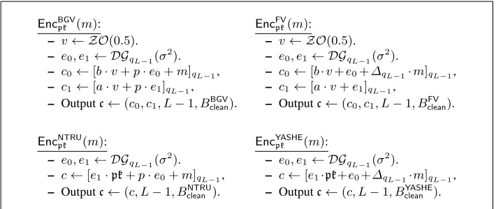
The encryption algorithms for all four schemes are given in Fig. 1. As for key generation we select slightly simpler distributions than the theory would imply so as to ensure noise growth is not as bad as it would otherwise be. The output of each algorithm is a tuplec consisting of the ciphertext data, the current level, plus a bound on the current “noise”

EncBGVpk (m):

– v← ZO(0.5). – e0, e1← DGq_L−1(σ

2₎

. – c0←[b·v+p·e0+m]qL−1,

– c1←[a·v+p·e1]qL−1,

– Outputc←(c0, c1, L−1, BcleanBGV).

EncNTRUpk (m):

– e0, e1← DGqL−1(σ

2_).

– c←[e1·pk+p·e0+m]qL−1,

– Outputc←(c, L−1, BcleanNTRU).

EncFVpk(m):

– v← ZO(0.5). – e0, e1← DGq_L−1(σ

2₎

.

– c0←[b·v+e0+∆qL−1·m]qL−1,

– c1←[a·v+e1]qL−1,

– Outputc←(c0, c1, L−1, BcleanFV ).

EncYASHEpk (m):

– e0, e1← DGqL−1(σ

2_).

– c←[e1·pk+e0+∆qL−1·m]qL−1,

– Outputc←(c, L−1, BYASHEclean ).

Fig. 1:Encryption Algorithms for BGV, FV, NTRU and YASHE

To understand the critical quantity we have to first look at the decryption procedure in each case. Then we can apply our heuristic noise analysis to obtain an upper bound on the canonical embedding norm of the critical quantity for a fresh ciphertext, and so obtainB∗_clean; a process which is done in the Appendix.

DecBGVpk (c): Decryption of a ciphertext(c0, c1, t, ν)at levelt is performed by setting

m0 ← [c0−sk·c1]qt, and outputtingm

0_{modp. If we define the critical quantity to}

bec0−sk·c1 (modqt), then this procedure will work whenνis an upper bound on the canonical embedding norm of this quantity andcm·ν < qt/2. Ifν satisfies this inequality then the value ofc0−sk·c1 (mod qt) will be produced exactly with no wrap-around, and will hence be equal tom+p·v, ifc0=sk·c1+p·v+m (modqt). Thus we must pick the smallest primeq0 =p0large enough to ensure that this always holds.

DecFVpk(c): Decryption of a ciphertext(c0, c1, t, ν)at leveltis performed by setting

m0←lp

qt

·[c0−sk·c1]qt

k ,

and outputtingm0modp. Consider the value of[c0−sk·c1]qt computed during

de-cryption, suppose this is equal to (over the integers before reduction modqt)m·∆qt+

w+r·qt. Then another way of looking at decryption is that we perform rounding on the value

p·∆qt·m

qt

+p·w qt

+p·r·qt qt

= p·(

qt

p −qt)·m

qt

+p·w qt

+p·r

=m+p·w−qt·m

qt

+p·r

w−qt·m

can

∞. The decryption procedure will then work whencm·ν < ∆qt/2, since

in this case we have

p·

w−qt·m

qt

_∞≤

cm·p

qt

·w−qt·m

can

∞ ≤

∆qt·p

2·qt

<1 2.

Thus again we must pick the smallest prime q0 = p0 large enough, to ensure that

cm·ν < ∆qt/2.

DecNTRU_pk (c): Decryption of a ciphertext(c, t, ν)at leveltis performed by settingm0←

[c·sk]qt, and outputtingm

0_{modp. Much as with BGV the critical quantity is[c·sk]} qt.

Ifν is an upper bound on the canonical embedding norm ofc·sk, and we havec = a·pk+p·e+mmoduloqt, for some values ofaande, then over the integers we have

[c·sk]qt =m+p·(a·g+e+f·m) +p

2 ·e·f,

which will decrypt tom. Thus for decryption to work we require thatcm·ν < qt/2.

DecYASHE_pk (c): Decryption of a ciphertext(c, t, ν)at leveltis performed by setting

m0←lp

qt

·[c·sk]qt

k ,

and outputtingm0modp. Following the same reasoning as for the FV scheme, suppose

c·skis equal to (again over the integers before reduction modqt)m·∆qt+w+r·qt.

Then for decryption to work we requireν to be an upper bound onw−qt ·m

can

∞ andcm·ν < qt/2.

3.3 Scale

These operations scale a ciphertext, reducing the corresponding level and more impor-tantly scaling the noise. The syntax is Scale∗(c, tout)wherecis at level tin and the output ciphertext is at level tout withtout ≤ tin. The noise is scaled by a factor of approximatelyqtin/qtout, however an additive term ofB

∗

scaleis added. For each of our

variants see the Appendix for a justification of the proposed method and an estimate on

B∗

scale.

For use in one of theSwitchKey∗variants we also use a Scale which takes a cipher-text with respect to modulusQand produces a ciphertext with respect to modulusq, whereq|Q. The syntax for this isScale∗(c, Q); the idea here is thatQis a “temporary” modulus unrelated to the actual leveltof the ciphertext, and we aim to reduceQdown toqt. The former scale function can be defined in terms of the latter via

Scale∗(c, tout):

– Writec= (c, t, ν).

ScaleBGV(c, Q):

– Writec= ((c0, c1), t, ν).

– Fixδi such that δi ≡ −ci (modP)

andδi≡0 (modp). – Writec0i←(ci+δi)/P. – ν0←ν/P+BBGV

scale. – Output((c00, c01), t, ν0).

ScaleNTRU(c, Q): – Writec= (c, t, ν).

– Fixδsuch thatδ ≡ −c (modP)and δ≡0 (modp).

– Writec0←(c+δ)/P. – ν0←ν/P+BNTRU

scale . – Output(c0, t, ν0).

ScaleFV(c, Q):

– Writec= ((c0, c1), t, ν).

– Fixδisuch thatδi≡ −ci (modP). – Writec0i←(ci+δi)/P.

– ν0←ν/P+BFVscale. – Output((c00, c

0

1), t, ν

0

).

ScaleYASHE₍

c, Q): – Writec= (c, t, ν).

– Fixδsuch thatδ≡ −c (modP). – Writec0←(c+δ)/P.

– ν0←ν/P+BYASHE Scale . – Output(c0, t, ν0).

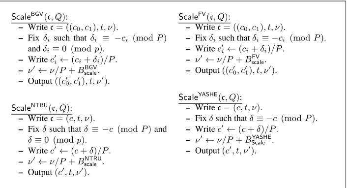
Fig. 2:Scale Algorithms for BGV, FV, NTRU and YASHE. In all methodsQ=qt·P, and for the BGV and NTRU schemes we assume thatP ≡1 (modp).

TheScale∗function was originally presented in [3] as a form of noise control for the non-scale invariant schemes. However, the use of such a function within the scale invariant schemes can also provide more efficient schemes, as alluded to in [6]. This is due to the modulus one is working with which decreases as homomorphic operations are applied. It is also needed for our second key switching variant. We thus present a

Scale∗function for all our four schemes in Fig. 2.

3.4 Reduce Level

For all schemes we can define aReduceLevel∗ operation which reduces a ciphertext level from levelt0 to leveltwheret0 ≥ t. For the non-scale invariant schemes when we reduce a level we only perform a scaling (which could be an expensive operation) if the noise is above some global bound B. This is because for small noise we can easily reduce the level by just dropping terms off the modulus, since the modulus is a product of primes. For the scale invariant schemes we actually need to perform aScale

operation since we need to modify the∆qt term. See the Appendix for details. In our

parameter estimation evaluation we examine the case, for FV and YASHE, of applying modulus switching to reduce levels and not applying it. In the case of not applying it all ciphertexts remain at levelL−1, andReduceLevel∗becomes a NOP.

3.5 Switch Key

– One based on decomposition modulo a general modulusT. See [11] for this method explained in the case of the BGV scheme. Unlike prior work we do not takeT = 2, as we treatT as a parameter to be optimized to achieve the most efficient scheme. Although to ease parameter search we restrict toTbeing a power of two.

– Our second method is based on the raising the modulus idea from [9], where it was applied to the BGV scheme. Here we adopt a more complex switching opera-tion, and a potentially larger parameter set, but we gain by reducing the size of the switching “matrices”.

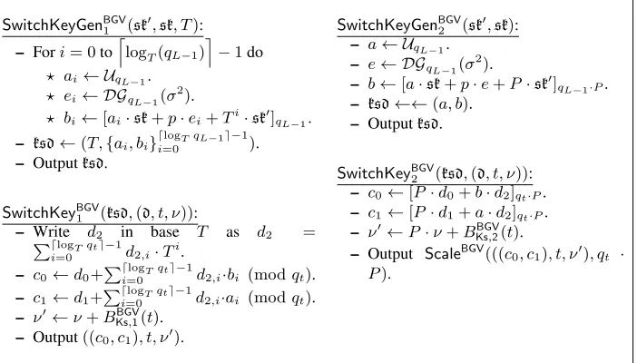
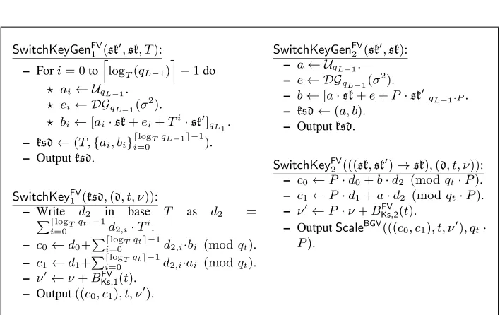
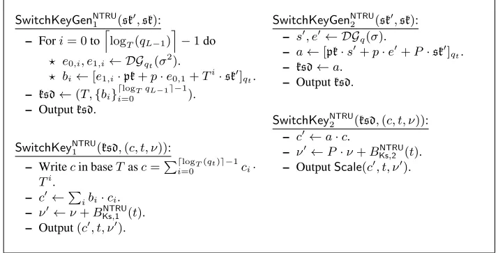
For each variant we require algorithmsSwitchKeyGenandSwitchKey; the first gener-ates the public switching “matrix”, whilst the second performs the actual switch key. In the BGV and FV schemes we perform a general key switch of the underlying decryp-tion equadecryp-tion of the formd0−sk·d1+sk0·d2 −→ c0−sk·c1. For the NTRU and YASHE schemes the underlying key switch is of the formc·sk0 −→ c0·sk. In Fig. 3 we present the key switching methods for the BGV algorithm. See the Appendix for the methods for the other schemes, plus derivations of upper bounds on the constants

BKs,∗∗(∗).

SwitchKeyGenBGV

1 (sk

0 ,sk, T): – Fori= 0tollogT(qL−1)

m

−1do ? ai← UqL−1.

? ei← DGq_L−1(σ2).

? bi←[ai·sk+p·ei+Ti_·sk0

]qL−1.

– ksd←(T,{ai, bi}dlogTqL−1e−1

i=0 ).

– Outputksd.

SwitchKeyBGV1 (ksd,(d, t, ν)):

– Write d2 in base T as d2 =

PdlogTqte−1

i=0 d2,i·Ti. – c0←d0+P

dlogTqte−1

i=0 d2,i·bi (modqt).

– c1←d1+P

dlogTqte−1

i=0 d2,i·ai (modqt).

– ν0←ν+BKsBGV,1(t). – Output((c0, c1), t, ν0).

SwitchKeyGenBGV

2 (sk

0 ,sk): – a← Uq_L−1.

– e← DGq_L−1(σ

2

).

– b←[a·sk+p·e+P·sk0]qL−1·P.

– ksd←←(a, b). – Outputksd.

SwitchKeyBGV₂ (ksd,(d, t, ν)): – c0←[P·d0+b·d2]qt·P.

– c1←[P·d1+a·d2]qt·P.

– ν0←P·ν+BBGVKs,2(t).

– Output ScaleBGV(((c0, c1), t, ν0), qt ·

P).

Fig. 3:The two variants of Key Switching for BGV.

In the context of BGV the first method requires us to storelogT(qL−1) “encryp-tions” ofsk0, each of which is an element inR2qL−1. The second method requires us to

store a single “encryption” ofP·sk0, but this time as an element inR2

P·qL−1. The

for-mer will require more space than the latter as soon aslog2P < logT(qL−1). In terms of noise the output noise of the first method is modified by an additive constant of

BKsBGV,1(t) = 8

√

3 ·p· l

logTqt

m

whilst the output noise of the second method is modified by the additive constant

BBGV Ks,2(t)

P +B

∗

scale=

8·p·qt·σ·φ(m) √

3·P +B

∗

scale.

As the level decreases this becomes closer and closer to B_scale∗ , as theP in the de-nominator will wipe out the numerator term. Thus the noise will grow of the order of

O(pφ(m))using the second method and asO(φ(m))using the first method. A sim-ilar outcomes arises when comparing the two methods with respect to the other three schemes.

3.6 Addition and Multiplication

We can now turn to presenting the homomorphic addition and multiplication operations. For reasons of space we give the addition and multiplication methods in the Appendix. In all methods the input ciphertextscihave levelti, and recall our parameters are such that we can evaluate circuits with multiplicative depthL−1.

3.7 Security and Parameters

In this section we outline how we select parameters in the case whereReduceLevel∗

is not a NOP (a no-operation). An analysis, for the FV and YASHE schemes, where

ReduceLevel∗ is a NOP we defer the analysis to the Appendix. We let B denote an upper bound onν at the output of anyReduceLevel∗operation. Following [9] we set

B= 2·B_scale∗ . We assume that operations are performed as follows. We encrypt, perform up toζadditions, then do a multiplication, then doζadditions, then do a multiplication and so on, where we assume decryption occurs after a multiplication.

Security: We assume, as a heuristic assumption, that if we set the parameters of the ring and modulus as per the BGV scheme then the other schemes will also be secure. We follow the analysis in [9], which itself follows on from the analysis by Lindner and Peikert [13]3_{. We therefore have one of two possible lower bounds forφ(m), for}

security parameterk

φ(m)≥



 

 

log(qL−1/σ)·(k+110)

7.2 If the first variant ofSwitchKeyis used,

log(P·qL−1/σ)·(k+110)

7.2 If the second variant ofSwitchKeyis used. (1)

Note thelogs here are natural logarithms.

Bottom Modulus: To ensure decryption correctness at level zero we require that

4·cm·B∗scale= 2·cm·B <



  

  

p0 For BGV and NTRU

j_p 0

p

k

For FV and YASHE.

(2)

3

Top Modulus: At the top level we take as input a ciphertext with noiseB_clean∗ , perform

ζ additions to produce a ciphertext with noise B1 = ζ·Bclean∗ . We then perform a

multiplication to produce something with noise

B2=



 

 

F∗(B1, B1) +BKs∗,1(L−1) If the first variant ofSwitchKeyis used,

F∗_(B

1, B1) + B∗

Ks,2(L−1)

P +B

∗

scale If the second variant ofSwitchKeyis used.

We then scale down a level to obtain something at the next level down. Thus we obtain something with noise bounded byB3 = _pB2

L−1 +B

∗

scale. We require, for our invariant, B3≤B= 2·B∗scale. Thus we require,

pL−1≥

B2

B∗

scale

. (3)

Middle Moduli: A similar argument applies for the middle moduli, but now we start off with a ciphertext with boundB = 2·B_scale∗ as opposed toB_clean∗ . Thus we form

B0(t) = 

 

 

F∗(ζ·B, ζ·B) +B∗_Ks,1(t) First variant ofSwitchKey,

F∗(ζ·B, ζ·B) +B ∗

Ks,2(t)

P +B

∗

scale Second variant ofSwitchKey.

after which aScaleoperation is performed. Hence, the moduluspt fort 6= 0, L−1 needs to be selected so that

pt≥

B0(t) B∗

scale

. (4)

Note, in practice we can do a bit better in the second variant ofSwitchKeyby merging the final two final scalings into one.

Putting It All Together: We are looking for parameters which satisfy equations (1), (2), (3) and (4), and which also minimize the size of data being processed, which is

φ(m)· L−1

X

t=0

pt

!

.

To do this we iterate through all possible values oflog2qL−1andlog2T(resp.log2P). We then determineφ(m), as the smallest value which satisfies equation (1). Here, we might need to take a larger value than the right hand side of equation (1) due to appli-cation requirements onpor the amount of packing required.

We then determine the size ofpL−1from equation (3), via

pL−1≈

l B₂ B∗_scale

We can now iterate downwards fort=L−2, . . . ,1by determining the size oflog₂qt, via

log₂qt= log2qt+1−log2pt+1.

If we obtainlog₂qt<0then we abort, and pass to the next pair of(log2qL−1, T)(resp.

(log₂qL−1,log2P)) values. The value ofptbeing determined by equation (4), via

pt≈

lB0(t) B_scale∗ m

.

Finally we check whether a primep0the size oflog2q0, will satisify equation (2), if so we accept this set of values as a valid set of parameters, otherwise we pass to the next pair of(log₂qL−1, T)(resp.(log2qL−1,log2P)) values.

0 2 4 6 8 10 12 14 4.5

5 5.5 6 6.5 7

log2(p)

log

2

(

|

c

|

)

kBytes

BGV, KS=1 BGV, KS=2 FV, KS=1 FV, KS=2 NTRU, KS=1 NTRU, KS=2 YASHE, KS=1 YASHE, KS=2

0 50 100 150 200 250 6

8 10 12 14 16

log2(p)

log

2

(

|

c

|

)

kBytes

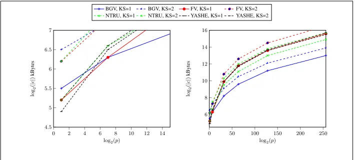
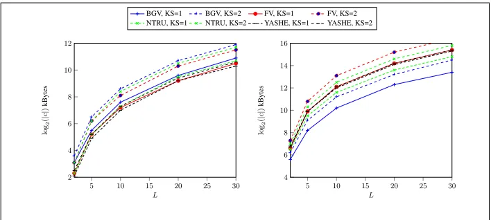
Fig. 4:Size of required ciphertext for various sizes of plaintext modulus whenL= 5. The graph on the left zooms into the portion of the right graph for small values oflog₂p.

4

Results

In the Appendix one can find a full set of parameters for each scheme, and variant of key switching, for various values of the plaintext moduluspand the number of levels

0 2 4 6 8 10 12 14 10

11 12 13

log2(p)

log

2

(

|

c

|

)

kBytes

BGV, KS=1 BGV, KS=2 FV, KS=1 FV, KS=2 NTRU, KS=1 NTRU, KS=2 YASHE, KS=1 YASHE, KS=2

0 50 100 150 200 250 10

12 14 16 18 20

log2(p)

log

2

(

|

c

|

)

kBytes

Fig. 5:Size of required ciphertext for various sizes of plaintext modulus whenL= 30. The graph on the left zooms into the portion of the right graph for small values oflog₂p.

For all schemes we used a Hamming weight ofh= 64to generate the secret key data, we used a security level ofk= 80bits of security, a standard deviation ofσ= 3.2

for the rounded Gaussians, a tolerance factor ofζ= 8and a ring constant ofcm= 1.3. These are all consistent with the prior estimates for parameters given in [9]. The use of a small ring constant can be justified by either selectingφ(m)to be a power of two, or selectingmto be prime, as explained in [4]. As a general conclusion we find that for FV and YASHE the use of modulus switching to lower levels results in slightly bigger parameters to start for large values ofL; approximately a factor of two forL= 20or30. But as a homomorphic calculation progresses this benefit will drop away, leaving, for most calculations, the variant in which modulus switching is applied the most efficient. Thus in what follows we assume that modulus switching is applied in all schemes.

Firstly examine the graphs in Figures 4 and 5. We see that for a fixed number of levels and very small plaintext moduli the most efficient scheme seems to be YASHE. However, quite rapidly, as the plaintext modulus increases the BGV scheme quickly outperforms all other schemes. In particular for the important case of the SPDZ MPC system [4] which requires an SHE scheme supporting circuits of multiplicative depth one, i.e.L= 2, for a large plaintext modulusp, the BGV scheme is seen to be the most efficient.

Examining Fig. 6 we see that if we fix the prime and just increase the number of levels then the choice of which is the better scheme is be very consistent. Thus one is led to conclude that the main choice of which scheme to adopt depends on the plaintext modulus, where one selects YASHE for very small plaintext moduli and BGV for larger plaintext moduli.

Acknowledgements

agree-5 10 15 20 25 30 2

4 6 8 10 12

L

log

2

(

|

c

|

)

kBytes

BGV, KS=1 BGV, KS=2 FV, KS=1 FV, KS=2 NTRU, KS=1 NTRU, KS=2 YASHE, KS=1 YASHE, KS=2

5 10 15 20 25 30 4

6 8 10 12 14 16

L

log

2

(

|

c

|

)

kBytes

Fig. 6:Size of required ciphertext for various values of L whenp= 2andp≈232_.

ment number ICT-644209. The authors would like to thank Steven Galbraith for com-ments on an earlier version of this manuscript.

References

1. J. W. Bos, K. E. Lauter, J. Loftus, and M. Naehrig. Improved security for a ring-based fully homomorphic encryption scheme. In M. Stam, editor,Cryptography and Coding - 14th IMA International Conference, IMACC 2013, Oxford, UK, December 17-19, 2013. Proceedings, volume 8308 ofLecture Notes in Computer Science, pages 45–64. Springer, 2013.

2. Z. Brakerski. Fully homomorphic encryption without modulus switching from classical gapsvp. In Safavi-Naini and Canetti [16], pages 868–886.

3. Z. Brakerski, C. Gentry, and V. Vaikuntanathan. Fully homomorphic encryption without bootstrapping. InInnovations in Theoretical Computer Science (ITCS’12), 2012. Available athttp://eprint.iacr.org/2011/277.

4. I. Damg˚ard, V. Pastro, N. P. Smart, and S. Zakarias. Multiparty computation from somewhat homomorphic encryption. In Safavi-Naini and Canetti [16], pages 643–662.

5. Y. Dor¨oz, Y. Hu, and B. Sunar. Homomorphic AES evaluation using the modified LTV scheme.Des. Codes and Cryptography, XXXX:XXXX–XXXX, 2015.

6. J. Fan and F. Vercauteren. Somewhat practical fully homomorphic encryption.IACR Cryp-tology ePrint Archive, 2012:144, 2012.

7. C. Gentry.A fully homomorphic encryption scheme. PhD thesis, Stanford University, 2009. crypto.stanford.edu/craig.

8. C. Gentry, S. Halevi, and N. Smart. Fully homomorphic encryption with polylog over-head. InEUROCRYPT, volume 7237 ofLecture Notes in Computer Science, pages 465–482. Springer, 2012. Full version athttp://eprint.iacr.org/2011/566.

9. C. Gentry, S. Halevi, and N. P. Smart. Homomorphic evaluation of the AES circuit. In Safavi-Naini and Canetti [16], pages 850–867.

11. K. Lauter, M. Naehrig, and V. Vaikuntanathan. Can homomorphic encryption be practical? InCCSW, pages 113–124. ACM, 2011.

12. T. Lepoint and M. Naehrig. A comparison of the homomorphic encryption schemes FV and YASHE. In D. Pointcheval and D. Vergnaud, editors,Progress in Cryptology -AFRICACRYPT 2014 - 7th International Conference on Cryptology in Africa, Marrakesh, Morocco, May 28-30, 2014. Proceedings, volume 8469 ofLecture Notes in Computer Sci-ence, pages 318–335. Springer, 2014.

13. R. Lindner and C. Peikert. Better key sizes (and attacks) for lwe-based encryption. In CT-RSA, volume 6558 ofLecture Notes in Computer Science, pages 319–339. Springer, 2011. 14. A. L`opez-Alt, E. Tromer, and V. Vaikuntanathan. On-the-fly multiparty computation on the

cloud via multikey fully homomorphic encryption. InSTOC. ACM, 2012.

15. V. Lyubashevsky, C. Peikert, and O. Regev. On ideal lattices and learning with errors over rings. InEUROCRYPT, volume 6110 ofLecture Notes in Computer Science, pages 1–23, 2010.

16. R. Safavi-Naini and R. Canetti, editors. Advances in Cryptology - CRYPTO 2012 - 32nd Annual Cryptology Conference, Santa Barbara, CA, USA, August 19-23, 2012. Proceedings, volume 7417 ofLecture Notes in Computer Science. Springer, 2012.

17. N. P. Smart and F. Vercauteren. Fully homomorphic SIMD operations.Des. Codes Cryptog-raphy, 71(1):57–81, 2014.

A

Estimating

B

BBGV

clean: The initial value ofνfor a fresh ciphertext isBcleanBGV, where our invariant is thatν

is an upper bound on the canonical embedding norm of the valuec0−sk·c1 (modqt). We have, using our above estimates for bounding the norm of random variables, for a fresh ciphertext,

c0−sk·c1

can

∞ =

((a·s+p·e)·v+p·e0+m−(a·v+p·e1)·sk

can

∞

=m+p·(e·v+e0−e1·sk)

can

∞

≤ m

can

∞ +p·

e·v can

∞ +

e0

can

∞ +

e1·sk

can

∞

≤p·p3·φ(m) +16·σ√·φ(m)

2

+ 6·σ·pφ(m) + 16·σ·ph·φ(m)

=B_cleanBGV.

BFV

clean: For a fresh ciphertext we need to upperbound the canonnical embedding of w−qt·m, namelyv·e+e0+e1·sk−qL−1·m. We have

w−qL−1·m

can

∞ ≤p·

m

can

∞ +

v·e

can

∞ +

e0

can

∞ +

e1·sk

can

∞ ≤p·p3·φ(m)

+16·σ√·φ(m)

2 + 6·σ· p

≤p·p

3·φ(m)

+ 2·σ·8·√φ(m)

2 + 3· p

φ(m) + 8·ph·φ(m)

=BFV_clean.

Note, compared to theBBGV

cleanwe do not have a dependence onpin the latter terms, but

we still have a dependence onpin the first term.

BNTRU

clean : For a fresh ciphertext we have, assumingpkis distributed as a uniformly

ran-dom element inAqt,

c·sk

can

∞ =

e1·pk·sk+ (p·e0+m)·(1 +p·f)

can

∞ ≤p·

e1·g

can

∞ +p·

e0

can

∞ +

m

can

∞

+p2· e0·f

can

∞ +p·

m·f

can

∞

≤16·p·σ·ph·φ(m) + 6·p·σ·pφ(m) +p·p3·φ(m)

+ 16·p2·σ·ph·φ(m) + 16·p2·ph·φ(m)/12

=

16·p·(1 +p)·σ+√8

3·p

2

·ph·φ(m)

+p·(6·σ+√3)·pφ(m)

=BNTRU_clean .

BYASHE

clean : For a fresh ciphertext we have that

w−qL−1·m= (e1·pk+e0)·sk−qL−1·m

=e1·p·g+e0·sk−qL−1·m.

Hence, we have

w−qL−1·m

can

∞ ≤

m

can

∞ +p·

e1·g

can

∞

+e0·(1 +p·f)

can

∞ ≤p·p3·φ(m) +p·16·σ·ph·φ(m)

+e0

can

∞ +p·

e0·f

can

∞ ≤p·p3·φ(m) + 16·p·σ·ph·φ(m)

+ 6·σ·pφ(m) + 16·p·σ·ph·φ(m)

= (6·σ+p·√3)·pφ(m) + 32·p·σ·ph·φ(m)

B

Estimating

B

ScaleBGV(c, Q): For correctness of the method presented we appeal to the proof of Lemma 13 in the full version of [8]. Basically the idea is that we have thatc0−sk·c1=

m+p·v+Q·u. Now adding onδ0−sk·δ1to both sides makes no difference modulo

p, sinceδi ≡ 0 (modp). In addition it makes the left hand side divisible exactly by

P over the integers. When dividing byP we do not affect the output modulop, since

P ≡1 (modp).

If we let (τ0, τ1) denote the rounding error τi = c0i −ci/P = δi/P, then the coefficients ofτi will behave as if they are drawn from a uniform distribution modulo

p. We then have that

c00−sk·c01

can

∞ =

1 P ·

c0−sk·c1+δ0−sk·δ1

can

∞

≤ ν

P +

τ0−sk·τ1

can

∞

≤ ν

P +

τ0

can

∞ +

sk·τ1

can

∞.

Thus we set

B_scaleBGV= 6·p·pφ(m)/12 + 16·p·pφ(m)·h/12

=p·p3·φ(m) + 8·pφ(m)·h/3.

ScaleFV(c, Q): We assume thatQ=qt·P, note we make no assumption onP. To show correctness we supposecdecrypts correctly moduloQ, i.e. ifc= ((c0, c1), t, ν)then

c0−sk·c1=m·∆Q+w+r·Q

where

∆Q=

jQ

p k

=Q

p −Q= qt·P

p −Q =P·(∆qt+qt)−Q

and

w−Q·m

can

∞ ≤ν.

The output ciphertext satisfies

c0₀−sk·c0₁= 1 P ·

c0+δ0−sk·c1−sk·δ1

= 1 P ·

m·∆Q+w+r·qt·P+δ0−sk·δ1

=∆qt·m+r·qt+qt·m+

1 P

−Q·m+w+δ0−sk·δ1

=∆qt·m+r·qt+w

As the left hand side is exactly divisible byP, and hence so must the right hand side be. To bound the noise of the output ciphertext we need to bound

w0−qt·m

can ∞ =

qt·m+

1 P

−Q·m+w+δ0−sk·δ1

−qt·m

can ∞ = 1 P ·

w−Q·m+δ0−sk·δ1

can ∞ ≤ 1 P ·

ν+δ0

can

∞ +

sk·δ1

can ∞ ≤ 1 P ·

ν+P·p3·φ(m) + 16·P·ph·φ(m)/12.

Thus

BFV_scale=p3·φ(m) + 8·p

h·φ(m)/3.

ScaleNTRU(c, Q): For showing correctness we note that we havec·sk=m+p·v+Q·u. Addingδ·skto both sides make no difference to the value modulop, asδ≡0 (modp)

and in addition it makes the left hand side divisible byP. When dividing byP we do not affectm (mod p)sinceP ≡1 (modP).

All that remains is to establish the value ofB_scaleNTRU. We let τ denote the round-ing errorτ = c0 −c/P = δ/P. The coefficients of τ will act like they are drawn from a uniform distribution modulo p, since the coefficients of δ are in the range

[−p·P/2, . . . , p·P/2]. We then have that

c0·sk

can ∞ = 1

P ·(c·sk+δ·sk) can ∞ ≤ ν P + τ·sk

can

∞

= ν

P +

τ·(1 +p·f) can ∞ ≤ ν P + τ can ∞ +

p·τ·f can

∞

≤ ν

P + 6·p· p

φ(m)/12 + 16·p2·ph·φ(m)/12

= ν P +p·

p

3·φ(m) +√8

3 ·p

2

·ph·φ(m)

= ν P +B

NTRU scale .

ScaleYASHE(c, Q): To show correctness we assume thatc= (c, t, ν)decrypts correctly moduloQ, i.e. we havec·sk=m·∆Q+w+r·Q, where∆Qis as above and

w−Q·m

can

∞ ≤ν.

We then have that

c0·sk= 1

= 1

P ·(m·∆Q+w+r·Q+δ·sk)

=m·∆qt+r·qt+m·qt+

1

P ·(w+δ·sk−m·Q) =m·∆qt+r·qt+w

0_.

To bound the noise of the output ciphertext we need to bound

w0−m·qt

can ∞ ≤

m·qt+

1

P(w+δ·sk−m·Q)−m·qt

can ∞ ≤ 1 P ·

w+δ·sk−m·Q can ∞ ≤ 1

P · ν+ δ·sk

can

∞

≤ 1

P · ν+

δ·(1 +pf) can

∞

≤ 1

P · ν+ δ

can

∞ +p·

δ·f

can ∞ ≤ 1 P ·

ν+P·p3·φ(m) + 16·P·pph·φ(m)/12

= ν

P +

p

3·φ(m) +√8

3 ·p· p

h·φ(m)

= ν P +B

YASHE Scale ,

on lettingBYASHE Scale =

p

3·φ(m) +√8 3·p·

p

h·φ(m).

C

Reduce Level

TheReduceLevel∗operations for our four schemes are presented in Fig. 7.

D

Switch Key

D.1 BGV

In each of the variants we switch from a keysk0 to a keysk. The input ciphertext will involve both keys; thus we aim a switch of the form

d0−sk·d1+sk0·d2−→c0−sk·c1.

For ease of reference we recap on the algorithms in Fig. 8.

SwitchKeyFirst Variant: This is the bit-decomposition method generalised for an ar-bitrary decomposition modulusT. We first establish that the output ciphertext encrypts the same message as the input ciphertext.

c0−sk·c1=d0+





dlogTqte−1

X

i=0

d2,i·bi



−d1·sk−sk·





dlogTqte−1

X

i=0

d2,i·ai



ReduceLevelBGV(((c00, c10), t0, ν), t):

– Ift0≤tthen abort. – Ifν > Bthen

? c←ScaleBGV_(((c0

0, c

0

1), t

0 , ν), t)

– Else

? c0 ←c00 (modqt).

? c1 ←c01 (modqt).

? c←((c0, c1), t, ν).

– Returnc.

ReduceLevelFV(((c00, c10), t0, ν), t):

– Ift0≤tthen abort.

– c←ScaleFV(((c00, c01), t0, ν), t)

– Returnc.

ReduceLevelNTRU((c0, t0, ν), t): – Ift0≤tthen abort. – Ifν > Bthen

? c←ScaleNTRU_((c0

, t0, ν), t)

– Else

? c←c0 (modqt). ? c←(c, t, ν). – Returnc.

ReduceLevelYASHE_((c0

, t0, ν), t): – Ift0≤tthen abort. – c←ScaleYASHE_((c0

, t0, ν), t)

– Returnc.

Fig. 7:TheReduceLevel∗Operations for BGV, FV, NTRU and YASHE.

SwitchKeyGenBGV

1 (sk

0 ,sk, T): – Fori= 0tollogT(qL−1)

m

−1do ? ai← Uq_L−1.

? ei← DGq_L−1(σ

2

).

? bi←[ai·sk+p·ei+Ti·sk0]qL−1.

– ksd←(T,{ai, bi}dlogTqL−1e−1

i=0 ).

– Outputksd.

SwitchKeyBGV

1 (ksd,(d, t, ν)):

– Write d2 in base T as d2 =

PdlogTqte−1

i=0 d2,i·Ti. – c0←d0+P

dlog_Tqte−1

i=0 d2,i·bi (modqt).

– c1←d1+P

dlog_Tqte−1

i=0 d2,i·ai (modqt).

– ν0←ν+BKsBGV,1(t). – Output((c0, c1), t, ν0).

SwitchKeyGenBGV

2 (sk

0 ,sk): – a← Uq_L−1.

– e← DGq_L−1(σ

2₎

.

– b←[a·sk+p·e+P·sk0]qL−1·P.

– ksd←(a, b). – Outputksd.

SwitchKeyBGV2 (ksd,(d, t, ν)):

– c0←[P·d0+b·d2]qt·P.

– c1←[P·d1+a·d2]qt·P.

– ν0←P·ν+BBGV Ks,2(t). – OutputScaleBGV_(((c

0, c1), t, ν0), qt·

P).

=d0−d1·sk+

dlog_Tqte−1

X

i=0

(d2,i·bi−d2,i·ai·sk)

=d0−d1·sk+

dlogTqte−1

X

i=0

p·ei+Ti·sk0

·d2,i

=d0−d1·sk+d2·sk0+p·

dlog_Tqte−1

X

i=0

d2,i·ei.

So assuming no wrap around the two ciphertexts encrypt the same value. We also have, for the noise term, that

c0− ·skc1

can

∞ ≤

d0−d1·sk+d2·sk0

can

∞ +p·

dlog_Tqte−1

X

i=0

d2,i·ei

can

∞

≤ν+√16

12·p· l

logTqt

m

·σ·φ(m)·T.

So we set

B_KsBGV_,1(t) = √8

3 ·p· l

log_Tqt

m

·σ·φ(m)·T.

Note, that the size of this term depends on the size of the current modulusqtas well as

T.

SwitchKeySecond Variant: Our second variant uses the raising the modulus idea. A large primePis selected which is congruent to one modulop. Note that unlike [9] the keyswitch constantBBGV

Ks,2(t)is the additionbeforethe scaling takes place, thus it will

look larger than in [9].

Again, we establish that the output ciphertext encrypts the same message as the input ciphertext. We look at the ciphertext before the scaling operation.

c0−sk·c1=P·(d0−sk·d1) +b·d2−a·d2·sk

=P·(d0−sk·d1) +d2·(p·e+P·sk0)

=P·(d0−sk·d1+sk0·d2) +p·e·d2.

So we will encrypt the same thing as long as the noise termp·e·d2 does not create wrap around moduloP·qt. The largePis to cater for the large value ofd2. We have

c0−sk·c1

can

∞ ≤P·

d0−sk·d1+sk0·d2

can

∞ +p·

e·d2

can

∞

≤P·ν+√16

12·p·qt·σ·φ(m).

So we set

B_KsBGV_,2(t) = √8

D.2 FV

In each of the variants we switch from a keysk0 to a keysk. The input ciphertext will involve both keys; thus we aim a switch of the form

d0−sk·d1+sk0·d2−→c0−sk·c1.

The two variants are described in Fig. 9.

SwitchKeyGenFV1 (sk

0 ,sk, T): – Fori= 0to

l

log_T(qL−1)

m

−1do ? ai← UqL−1.

? ei← DGq_L−1(σ2_).

? bi←[ai·sk+ei+Ti·sk0]qL₁.

– ksd←(T,{ai, bi}dlogTqL−1e−1

i=0 ).

– Outputksd.

SwitchKeyFV

1 (ksd,(d, t, ν)):

– Write d2 in base T as d2 =

PdlogTqte−1

i=0 d2,i·Ti. – c0←d0+P

dlog_Tqte−1

i=0 d2,i·bi (modqt).

– c1←d1+P

dlog_Tqte−1

i=0 d2,i·ai (modqt).

– ν0←ν+BKsFV,1(t). – Output((c0, c1), t, ν0).

SwitchKeyGenFV2 (sk

0 ,sk): – a← UqL−1.

– e← DGq_L−1(σ2).

– b←[a·sk+e+P·sk0]qL−1·P.

– ksd←(a, b). – Outputksd.

SwitchKeyFV2 (((sk,sk

0

)→sk),(d, t, ν)): – c0←P·d0+b·d2 (modqt·P).

– c1←P·d1+a·d2 (modqt·P).

– ν0←P·ν+BKsFV,2(t).

– OutputScaleBGV(((c0, c1), t, ν0), qt·

P).

Fig. 9:The two variants of Key Switching for FV.

SwitchKeyFirst Variant: This is the bit-decomposition method generalised for an ar-bitrary decomposition modulust. Note that the(ai, bi)do not even “look like” encryp-tions ofTi·sk0in the FV scheme. As before, we first establish that the output ciphertext encrypts the same message as the input ciphertext. We writed0−d1·sk+d2·sk0 =

m·∆qt+w+r·qt

c0−sk·c1=d0+





dlogTqte−1

X

i=0

d2,i·bi



−d1·sk−sk·





dlogTqte−1

X

i=0

d2,i·ai





=d0−d1·sk+

dlog_Tqte−1

X

i=0

(d2,i·bi−d2,i·ai·sk)

=d0−d1·sk+

dlogTqte−1

X

i=0

ei+Ti·sk0

=d0−d1·sk+d2·sk0+

dlog_Tqte−1

X

i=0

d2,i·ei

=m·∆qt+w+r·qt+

dlogTqte−1

X

i=0

d2,i·ei

=m·∆qt+w

0_+r·q t.

So assuming no wrap around the two ciphertexts encrypt the same value. We also have, for the noise term, that

w0−qt·m

can

∞ ≤

w−qt·m

can

∞ +

dlogTqte−1

X

i=0

d2,i·ei

can

∞

≤ν+√16

12· l

log_Tqt

m

·σ·φ(m)·T.

So we set

BFV_Ks,1(t) =√8

3· l

log_Tqt

m

·σ·φ(m)·T.

Note, that the size of this term depends on the size of the current modulusqtas well as

T.

SwitchKey Second Variant: Our second variant uses the raising the modulus idea from [9], hence a large primeP is selected. Note as we are using a scale invariant version we do not requireP ≡1 (modp), and again note that(a, b)does not “look like” an encryption ofP·sk0. To establish that the output ciphertext encrypts the same message as the input ciphertext, we writed0−d1·sk+d2·sk0=m·∆qt+w+r·qt.

We look at the ciphertext before the scaling operation.

c0−sk·c1=P·(d0−sk·d1) +b·d2−a·d2·sk

=P·(d0−sk·d1) +d2·(e+P·sk0)

=P·(d0−sk·d1+sk0·d2) +e·d2

=P·(m·∆qt+w+r·qt) +e·d2

=m·P·∆qt+P·w+P·r·qt+e·d2

=m·(∆P·qt+Q−P·qt) +P·w+P·r·qt+e·d2

=m·∆P·qt+w

0_+r0_·q t

We have

w0= (Q−P·qt)·m+P·w+e·d2,

and we know by our invariant thatw−qt·m

can

∞ ≤ν. This leads us to consider the inequalities

w0−P·qt·m

can

∞ =

P·w−P·qt·m+e·d2

can

≤P·

w−qt·m

can

∞ +

e·d2

can

∞

≤P·ν+√16

12·qt·σ·φ(m).

So we set

B_KsFV_,2(t) = √8

3 ·qt·σ·φ(m).

D.3 NTRU

Letc0 be a ciphertext with respect to the secret key sk0. In both variants, we want to obtain a ciphertextcwith respect to another secret keysksuch that both decrypt to the same message. The two variants are described in Fig. 10.

SwitchKeyGenNTRU1 (sk

0 ,sk): – Fori= 0to

l

log_T(qL−1)

m

−1do ? e0,i, e1,i← DGqt(σ

2

).

? bi←[e1,i·pk+p·e0,1+Ti·sk0]qt.

– ksd←(T,{bi}dlogTqL−1e−1

i=0 ).

– Outputksd.

SwitchKeyNTRU1 (ksd,(c, t, ν)):

– Writecin baseTasc=PdlogT(qt)e−1

i=0 ci·

Ti. – c0←P

ibi·ci. – ν0←ν+BKsNTRU,1 (t). – Output(c0, t, ν0).

SwitchKeyGenNTRU2 (sk

0 ,sk): – s0, e0← DGq(σ).

– a←[pk·s0+p·e0+P·sk0]qt.

– ksd←a. – Outputksd.

SwitchKeyNTRU2 (ksd,(c, t, ν)):

– c0←a·c.

– ν0←P·ν+BKsNTRU,2 (t). – OutputScale(c0, t, ν0).

Fig. 10:The two variants of Key Switching for NTRU.

SwitchKeyFirst Variant: Recall we havepk= [p·g/sk]qt (seeKeyGen NTRU

) andc, sk0are such thatc·sk0 =m+p·e (modqt). we then see that

sk·c0=X

i

e1,i·pk+p·e0,i+Ti·sk0·ci·sk

=c·sk0·sk+p· X i

e1,i·g·ci+

X

i

e0,i·ci·sk

!

= (m+p·e)·(1 +p·f) +p· X i

e1,i·g·ci+

X

i

e0,i·ci·sk

=m+p· e+f·(m+p·e) +X

i

e1,i·g·ci+

X

i

e0,i·ci·sk

!

.

Thus assumingsk·c0

can

∞ is suitably small we will obtainmupon decryption. All that remains is to boundν0, by deriving an estimate forBNTRU

Ks,1 (t),

sk·c0

can ∞ = c·sk

0

·sk+p· X i

e1,i·g·ci+

X

i

e0,i·ci·sk

! can ∞ ≤ c·sk

0_+p·c·sk0_·f can ∞ + p· X i

e1,i·g·ci+

X

i

e0,i·ci+p·

X

i

e0,i·ci·f

! can ∞

≤ν+p·6·ν·√h+ 40·llog_T(qt)

m

·T·σ·φ(m)·ph/12

+ 16·llogT(qt)

m

·T·σ·φ(m)·p1/12

+ 40·p·llog_T(qt)

m

·T ·σ·φ(m)·ph/12

≤ν+p·6·ν·√h+√20

3 ·(1 +p)· l

log_T(qt)

m

·T·σ·φ(m)·√h

+√8

3· l

logT(qt)

m

·T·σ·φ(m).

So we let

B_KsNTRU_,1 (t) =p·6·ν·√h+√20

3·(1 +p)· l

log_T(qt)

m

·T ·σ·φ(m)·√h

+√8

3 · l

log_T(qt)

m

·T·σ·φ(m).

Note thatBNTRU

Ks,1 (t)depends onν, which is not the case for the BGV and FV schemes.

SwitchKeySecond Variant: Sincecdecrypts undersk0, letc·sk0 = m+p·e. We look at the ciphertext before the scaling operation, and see

c0·sk= (pk·s0+p·e0+P·sk0)·c·sk

=pk·s0·sk·c+ (p·e0+P·sk0)·c·(1 +p·f)

=P·sk0·c+p·g·s0·c+p·e0·c+p2·e0·c·f +p·P·sk0·c·f

Thus we will obtain, assuming no wrap around, the “message”P·m=mmodulop. To guarantee no wrap around we need to boundc0_·sk

can

∞

c0·sk

can

∞ =

P·sk

0_·c+p·g·s0_·c+p·e0_·c+p2_·e0_{·c·f+p·P·sk}0_·c·f

can

∞ ≤P·

c·sk0 can

∞ +p·

g·s0·c can

∞ +p·

e0·c

can

∞ +p 2_·

e0·c·f can

+p·P·

sk0·c·f

can

∞ ≤P·ν+ 40·p·qt·σ·φ(m)·

p h/12

+√8

3 ·p·qt·σ·φ(m)

+ 40·p2·qt·σ·φ(m)·

p h/12

+ 6·p·P·ν·√h

=P·ν+ 40·p·(1 +p)·qt·σ·φ(m)·

p h/12

+√8

3 ·p·qt·σ·φ(m)

+ 6·p·P·ν·√h.

Thus we set

BKsNTRU,2 (t) = 40·p·(1 +p)·qt·σ·φ(m)·

p

h/12 +√8

3·p·qt·σ·φ(m) + 6·p·P·ν·

√

h.

Note again thatBNTRU

Ks,2 (t)depends onν.

D.4 YASHE

Again letc0be a ciphertext with respect to the secret keysk0. In both variants, we want to obtain a ciphertextcwith respect to another secret keysksuch that both decrypt to the same message. The two variants are described in Fig. 11.

SwitchKeyGenYASHE1 (sk

0 ,sk): – Fori= 0tollog_T(qL−1)

m

−1do ? e0,i, e1,i← DGqt(σ

2

).

? bi←[e1,i·pk+e0,1+Ti·sk0]qt.

– ksd←(T,{bi}dlogT(qL−1)e−1

i=0 ).

– Outputksd.

SwitchKeyYASHE

1 (ksd, c, t, ν):

– ν0←ν+BYASHE Ks,1 (t).

– Writecin baseT asPdlogT(qt)e−1

i=0 ci·T

i . – Setc0=P

ibi·ci. – Outputc= (c0, t, ν0).

SwitchKeyGenYASHE2 (sk

0 ,sk): – e0, e1← DGq(σ).

– a←[pk·e1+e0+P·sk0]Q.

– ksd←a. – Outputksd.

SwitchKeyYASHE2 (ksd,(c, t, ν)):

– ν0←ν+BScaleYASHE. – d←a·c.

– c0←Scale(d, P, qt). – Outputc= (c0, ν0, t).

SwitchKeyFirst variant: Since we start with a ciphertextcwhich decrypts undersk0, letc·sk0=∆qt·m+w+r·qt. Then notice that

sk·c0=X

i

(e1,i·pk+e0,i+Ti·sk0)·ci·sk

=p·X i

e1,i·g·ci+

X

i

e0,i·ci·sk+c·sk0·sk

=p·X i

e1,i·g·ci+

X

i

e0,i·ci·sk+c·sk0·(1 +p·f)

=p·X i

e1,i·g·ci+

X

i

e0,i·ci·sk+ (∆qt·m+w+r·qt)

+p·f·(∆qt·m+w+r·qt)

=p·X i

e1,i·g·ci+

X

i

e0,i·ci·sk+ (∆qt·m+w+r·qt)

−p·f·m·qt−p·f·m·qt+p·f·(w+r·qt)

=∆qt·m+w

0_+r0_·q t,

where we havew0 =p·P

ie1,i·g·ci+

P

ie0,i·ci·sk−p·f·m·qt+w·(1 +p·f)

andr0=r·(1 +p·f) +p·f·m. We therefore want to bound

w0−qt·m

can

∞ ≤

p·X

i

e1,i·g·ci+

X

i

e0,i·ci·sk−p·f·m·qt

can

∞

+w·(1 +p·f)−qt·m

can

∞ ≤

w−qt·m

can

∞

+p·

X

i

e1,i·g·ci

can ∞ + X i

e0,i·ci·(1 +pf)

can

∞

−p·qt·

f·m

can

∞

+p· f·w

can

∞ ≤

w−qt·m

can

∞

+p· X

i

e1,i·g·ci

can ∞ + X i

e0,i·ci

can

∞

+p·

X

i

f ·e0,i·ci

can

∞

+p· f·m

can

∞

+p·f·(w−qt+qt)

can

∞ ≤ν+ 40·p· dlog_T(qt)e ·T·σ·φ(m)·

+ 16· dlog_T(qt)e ·σ·T·φ(m)·

p 1/12

+ 40·p· dlog_T(qt)e ·T ·σ·φ(m)·

p h/12

+ 16·p2·ph·φ(m)/12

+p·

f·(w−qt)

can

∞

+p· f·qt

can

∞

≤ν+√40

3 ·p· dlogT(qt)e ·T·σ·φ(m)·

√

h

+√8

3 · dlogT(qt)e ·T·σ·φ(m)

+√8

3 ·p

2_·p

h·φ(m)

+ 6·p·ν·√h

+ 6·p·√h

≤ν+√8

3 ·

1 + 5·p·√h· dlogT(qt)e ·T·σ·φ(m)

+√8

3 ·p

2_·p

h·φ(m)

+ 6·p·(ν+ 1)·√h.

LetBYASHE Ks,1 (t) =

8 √ 3·

1 + 5·p·√h·dlog_T(qt)e·T·σ·φ(m)+√8₃·p2·

p

h·φ(m)+

6·p·(ν+ 1)·√h. Note that as in the previous section, this depends onν.

SwitchKey Second Variant: Here again we use the idea of raising the modulus to some largeP, then use theScalefunction at the end of the operation. We letQ=qt·P

and recall that ∆Q =

j_Q

p

k

= Q_p −Q = qt_p·P −Q = P ·(∆qt +qt)−Q. We

first check that the output decrypts correctly. Sincecdecrypts undersk0, we have that

c·sk0=∆qt·m+w+r·qt.

d·sk=a·c·sk

=sk·(pk·e1+e0+P·sk0)·c

=P·sk·sk0·c+ (sk·e0+p·e2·g)·c

=P·sk·(∆qt·m+w+r·qt) + (sk·e0+p·e2·g)·c

=P·sk·∆qt·m+P·sk·(w+r·qt) + (sk·e0+p·e2·g)·c

=P·sk·m·∆qt+P·sk·(w+r·qt) + (sk·e0+p·e2·g)·c

= (1 +p·f)·m·P·∆qt+P·sk·(w+r·qt) + (sk·e0+p·e2·g)·c

=∆Q·m+m·(Q−P·qt) +p·f·m·P·∆qt

+P·sk·(w+r·qt) + (sk·e0+p·e2·g)·c

+P·(1 +p·f)·(w+r·qt) + (sk·e0+p·e2·g)·c

=∆Q·m+m·(Q−P·qt) +p·f·m·P·(

qt

p −qt)

+P·(w+r·qt) +p·f ·(w+r·qt) + (sk·e0+p·e2·g)·c

=∆Q·m+m·(Q−P·qt) +f ·m·Q−p·f ·m·P·qt

+P·(w+r·qt) +p·f ·(w+r·qt) + (sk·e0+p·e2·g)·c

=∆Q·m+w0+r0·Q,

wherew0=m·(Q−P·qt)−p·P·qt·f·m+P·w+p·f·w+ (sk·e0+p·e2·g)·c

andr0 = r+r·p·f +f ·m. Thus we indeed have a ciphertext moduloQwhich correctly decrypts to the initial messagem, so long as the noise is not too big. We know thatw−m·eqt

can

∞ ≤νand so we consider

w0−Q·m

can

∞ ≤

−p·P·qt·f·m+p·f·w+ (sk·e0+p·e2·g)·c

can

∞

+P·w+m·(Q−P·qt)−Q·m

can

∞ ≤

p·P·qt·f ·m

can

∞

+p·f·(w−qt·m+qt·m)

can

∞

+(1 +p·f)·e0·c

can

∞

+p·e2·g·c

can

∞

+P·w+m·Q−P·m·qt−Q·m

can

∞ ≤

p·P·qt·f ·m

can

∞

+p·f·(w−qt·m)

can

∞

+p·f·qt·m)

can

∞

+

(1 +p·f)·e0·c

can

∞

+p· e2·g·c

can

∞

+P·

w−m·qt

can

∞ ≤P·p·

f ·m can

∞

+p·ν· f

can

∞

+p2· f ·m)

can

∞

+e0·c

can

∞

+p·

f·e0·c

can

∞

+p·e2·g·c

can

∞

+P·ν

≤16·P·p2·ph·φ(m)/12

+ 6·p·ν·√h

+ 16·qt·σ·φ(m)/ √

12

+ 40·p·qt·σ·φ(m)·

p h/12

+ 40·p·qt·σ·φ(m)·

p h/12

+P·ν

≤√8

3·P·p

2_·p

h·φ(m)

+ 6·p·ν·√h

+√8

3 ·p

2_·p

h·φ(m)

+√8

3 ·qt·σ·φ(m)

+√40

3 ·p·qt·σ·φ(m)·

√

h

+P·ν

Therefore, we setBYASHE Ks,2 (t) =

8 √

3 ·P·p 2_·p

h·φ(m) + 6·p·ν·√h+√8 3 ·p

2_·

p

h·φ(m) +√8

3·qt·σ·φ(m) + 40 √

3·p·qt·σ·φ(m)· √

h. Again note this depends on the previous noise boundν.

E

Addition and Multiplication

The homomorphic addition method for all schemes is given in Fig. 12, whilst those for multiplication are given in Fig. 13.

E.1 BGV

These methods are standard. The fact that the output ciphertext satisfies c0 −sk ·

c1

can

∞ ≤νin both cases is obvious.

E.2 FV

To see that the outputν is correct for the addition operation, we writeci,0−sk·ci,1=

∆qt·mi+wi+ri·qtandc0−sk·c1 =∆qt·m+w+r·qt, wheremi∈Ap, and

writem= [m0+m1]p=m0+m1+p·ra. Then, decryptingcresults in the taking the value (moduloqt)

∆qt·(m0+m1) +w0+w1=∆qt·(m−p·ra) +w0+w1 (mod qt)

=∆qt·m+w0+w1−p·ra·∆qt

=∆qt·m+w0+w1−p·ra·

q_t p −qt

AddBGV(c0,c1):

– t= min(t0, t1).

– ci ← ReduceLevelBGV(ci, t) fori =

1,2.

– Writeci= (ci,0, ci,1, t, νi).

– c0 ←c0,0+c1,0 (modqt).

– c1 ←c0,1+c1,1 (modqt).

– ν←ν0+ν1

– Output((c0, c1), t, ν).

AddNTRU(c0,c1):

– t= min(t0, t1).

– ci ← ReduceLevelNTRU(ci, t)fori =

1,2.

– Writeci= (ci, t, νi). – c←c0+c1 (modqt).

– ν←ν0+ν1

– Output(c, t, ν).

AddFV(c0,c1):

– t= min(t0, t1).

– ci ← ReduceLevelFV(ci, t) for i =

1,2.

– Writeci= (ci,0, ci,1, t, νi).

– c0←c0,0+c1,0 (modqt).

– c1←c0,1+c1,1 (modqt).

– ν←ν0+ν1

– Outputc= ((c0, c1), t, ν).

AddYASHE(c0,c1):

– t= min(t0, t1).

– ci ←ReduceLevelYASHE(ci, t)fori=

1,2.

– Writeci= (ci, t, νi). – c←c0+c1 (modqt).

– ν←ν0+ν1

– Outputc= (c, t, ν).

Fig. 12:The Addition Methods for BGV, FV, NTRU and YASHE.

=∆qt·m+w

multiplying the result byp/qtand rounding. Thusw=w0+w1+p·ra·qtand so the

νvalue oncis an upper bound on

w−qt·m

can

∞ =

w0+w1+p·ra·qt−qt ·(m0+m1+p·ra)

can

∞ ≤

w0−qt·m0

can

∞ +

w1−qt·m1

can

∞ ≤ν0+ν1.

For the multiplication operation the tripled= (d0, d1, d2)decrypts via the equation

lp

qt

·[d0−sk·d1+sk2·d2]qt

k

which is why we need theSwitchKeyoperation. To establish correctness, and the bound onν, we write[ci,0−sk·ci,1]qt =∆qt·mi+wi+ri·qt. Recall that

wi−qt·mi

can

∞ ≤νi, which means that

wi can ∞ ≤

wi−qt·mi

can

∞ +

qt·mi

can

∞ ≤νi+p·

p

3·φ(m) =Bwi.

Note that this means that

ri can ∞ = 1 qt

(ci,0−sk·ci,1−∆qt·mi−wi)

can

MultBGV_(c

0,c1):

– t= min(t0, t1).

– ci ← ReduceLevelBGV(ci, t) fori =

1,2.

– Writeci= (ci,0, ci,1, t, νi).

– d0←c0,0·c1,0.

– d1←c0,0·c1,1+c0,1·c1,0.

– d2←c0,1·c1,1.

– d←(d0, d1, d2).

– ν←FBGV_(ν

0, ν1) =ν0·ν1.

– c←SwitchKeyBGV∗ (ksd,(d, t, ν)). – c←ReduceLevelBGV_{(c, t−1)}

.

MultNTRU_(c

0,c1):

– t= min(t0, t1).

– ci ← ReduceLevelNTRU(ci, t)fori =

1,2.

– Writeci= (c, t, νi). – d←c0·c1.

– ν←FNTRU_(ν

0, ν1) =ν0·ν1.

– c←SwitchKeyNTRU∗ (ksd,(d, t, ν)). – c←ReduceLevelNTRU_{(c, t−1).}

MultFV_(c

0,c1):

– t= min(t0, t1).

– ci←ReduceLevelFV(ci, t)fori= 1,2. – Writeci= (ci,0, ci,1, t, νi).

– d000 ←

p

qt ·(c0,0·c1,0).

– d001 ← qpt ·(c0,0·c1,1+c0,1·c1,0).

– d002 ←

p

qt ·(c0,1·c1,1).

– d00←

l

d000

k

, d01←

l

d001

k

, d02←

l

d002

k

. – d0←[d00]qt, d1←[d

0

1]qt, d2←[d

0

2]qt.

– d←(d0, d1, d2).

– ν←FFV_(ν

0, ν1).

– c←SwitchKeyFV∗ (ksd,(d, t, ν)). – c←ReduceLevelFV_{(c, t−1).}

MultYASHE_(c

0,c1):

– t= min(t0, t1).

– ci←ReduceLevelYASHE(ci, t)fori= 1,2. – Writeci= (ci, t, νi).

– d00← _qp

t ·(c0·c1).

– d0←ld00

k

. – d←[d0]qt.

– ν←FYASHE(ν0, ν1).

– c←SwitchKeyYASHE

∗ (ksd),(d, t, ν)). – c←ReduceLevelYASHE(c, t−1).