Volume 10, Number 3
I
Journal of
May, 1957RANGE
MANAGEMENT
“Water-Belly” (Urolithiasis) in Range Steers
in Relation to Some Characteristics
of Rangeland’
KARL G. PARKER
Extewsion Ratige Specialist, Mowhna State College, Boxeman, Montana
Water-belly, urinary calculi or urolithiasis, has caused widespread losses among cattle. Cattlemen in the Great Plains of the United States ranked water-belly second in occurrence among all nutrition- ally sick cattle in 1954 (Ensmin- ger, et al., 1955). In the western states, except the Great Plains, it ranked fifth, and in the southern states it ranked seventh.
Range operators think of water- belly as being strictly a range cat- tle problem. Livestock f eedlot operators think of it as being strictly a feed-lot problem. Actual- ly, it is common to both, but the majority of scientific investiga- tions into the problem have been on feedlot cattle.
This study follows the “range approach” to the problem. It was
1 Contribution from Montana State Col- lege Agricultural Experiment Station, Paper No. 397, Journal Series. This paper is adapted from the author’s Master of Science Thesis. The Thesis is available through interlibrary loan service from the Montana State College Library.
Acknowledgement is made to Dr. G. F. Payne and Dr. P. A. Branson, Depart- ment of Animal Industry and Range Management, Montama State College, for assistance during the study and in pre- paration of the manuscript.
undertaken to determine relation- ships of range vegetational types, range condition, range sites, the annual and seasonal incidence of the disease in cattle, and the min- eral content of range forages in relation to the incidence of water- belly. It was limited primarily to cattle and the range upon which they grazed. Another purpose of the study was to find practical means by which ranchers might reduce the extensive losses due to water-belly in range cattle.
The study covered a period of two winters, the winter of 1954-55 and the winter of 1955-56.
Mathams and Sutherland (1951) observed that cows coming to an Australian abatoir from the Gym- pie-Eumundi district had consider- able amounts of kidney stones. An- alysis showed these stones to be composed almost entirely of silica. Such instances occurred rarely in cattle from other districts. These workers indicated that pastures in the Gympie-Eumundi district have a great deal of “blady grass”,
(Imperata cylindrica major) in the pastures in which the affected cattle grazed. Swingle (1953) an- alyzed stones from 63 steers. All contained a high percentage of silica.
Jones, Black, Ellis, and Keating
105
(1949) of the Texas Agricultural Experiment Station recognized that urinary calculi condition of steers in feedlots was probably not due entirely to feedlot environ- ment. Madsen (1954), found a high but variable content of silica in certain harvested range forages collected in New Mexico and Texas. These and other workers have speculated on the presence of a re- lationship between the high silica intake from forage and soil and the later incidence of water-belly in steers on fattening rations. Silica is one of the most abundant single minerals of the soil (Byers, et al., 1938).
Relationships of mineral compo- sition of range plants to the sites in which they grow was suggested in a study by Gordon and Samp- son (1939). In their study, it was noted that low soil phosphorus re- sulted in low phosphorus and high potassium content of plants.
The actual metabolic changes undergone by minerals absorbed from plants by range cattle is not well understood and little research has been done along this line. A mineral balance type of metabo- lism experiment was conducted in Ohio by Forbes and Beegle (1916). The retention of silicon from ra- tions containing timothy hay and corn silage was surprisingly large.
The Study Arm
This study was conducted pri- marily in the southeastern one- fourth of Montana. The ranches studied were located in Rosebud, Musselshell, Carter, Carbon, and Wheatland Counties. Information from other areas in Montana, Colo- rado, and Utah was also obtained.
106
tion of the grassland formation. This association or type alternates with the desert shrub and salt desert shrub type. The latter type occupies a much smaller percent- age of the study area than does the former.
Most of the study area is in the 10 to 14 inch rainfall belt. South- ern Rosebud County is in the 15 to 19 inch rainfall belt. The pre- cipitation in the study area ranged from 8.49 inches to 13.33 inches in 1954, but in 1955 the precipitation was higher, ranging from 10.01 to 17.51 inches. Precipitation was about three inches below normal the first year of the study and two inches above normal the second year.
The average annual tempera- tures ranged from 41.5 degrees to 46.8 degrees Fahrenheit.
Methods and Procedure
Ranch units were studied in pairs in order to permit clear ex- pression of animal-soil-vegetation- water relationships. Two ranch units for a ‘pair were selected for comparable size, kinds of cattle, climatic conditions, and manage- ment. At the same time, these units were selected to provide a degree of contrast in their experi- ence with the incidence of water- belly.Ranches were visited and data obtained on cattle management, range vegetational types, range sites, range condition, and the inci- dence of water-belly. Composite samples of range forage plants, supplemental forages, and water utilized by the cattle during the fall and winter months were col- lected. The estimated utilization of the important range species was recorded at the time of the ranch visits. Practice in estimation of utilization and range condition was gained in a preparatory program which made use of exclosures and clip quadrats.
Range condition and site rela- tionships were determined on the basis of technician’s guides to range condition classes, and recom-
KARL G. PARKER
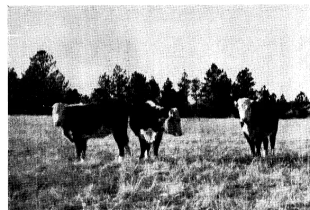
FIGURE 1. Steers grazing on high benches selected threndleaf sedge during December, - January, and February in the winter of 1954-55. Water-belly incidence was 28.6
percent in this herd.
mended stocking rates, prepared by the Soil Conservation Service.
A corollary study to obtain in- formation on the mineral compo- sition of the important range spe- cies was conducted over a period of one year bon a ranch near Ashland, Montana. Sampler of the impor- tant species were taken at two- week intervals May 1954 through January 1955 and once a month during February, March and April, 1955. Species sampled in- cluded western wheatgrass (&TO- pyron smithii) , bluebunch wheat- grass (Ayropyron spicatum) , blu!: grama (Bozcteloua gracilis) , June- grass (Icoeleria cristata), Sand- berg bluegrass ( POCF secunda) , needle-and-thread ($tipa comata), green needlegrass (Stipa viridula) and threadleaf sedge (Carex fiZ;- folia) .
Forage samples were analyzed by the Chemistry Department of the Montana Agricultural Experi- ment Station for moisture, protein, calcium, phosphorus, magnesium, silica, and for potassium on some samples. Water samples were an- alyzed for calcium, phosphorus and silica.
A mail survey of 24 ranches in the northern desert shrub-saltbush type of central Utah was con- ducted.
Results and Discussion
Vegetational Types and Incidence of Water-belly
Six vegetational types were en- countered on rangelands in this phase of the study. They are listed in Table 1.
Only three of twenty-one ranch units had cattle grazing on a single vegetational type. Thus, it was necessary to base this study on the complexes and transitions of type, instead of pure vegetational types. There was a total of 3,451 cattle on these ranch units. The minimum number of cattle grazed on any one of the six vegetational types was 198; the maximum number on any one type was 987.
Cattle herds on vegetational types containing only grass and unpalatable shrubs had ten times as much water-belly as herds on types containing shrubs that were palatable.
Four additional ranch units wintered steers on cultivated crops including cultivated hays and aftermath of legumes, together with small grain stubble. There was no water-belly among these 541 steers.
WATER-BELLY IN STEERS IN RELATION TO RANGE 107
Table 1. Range vegetational types in relation to the inddence of water-belly on selected ranch units in southeastern Montana; winters of 1954-55 and 195556.
Number of Number of Total
Ranch Units Water- Number Percent
In Which belly of Water-
Type Cases Cattle belly
Vegetational Types Occurred In Herds In Herds Incidence
Mixed grass-Savannah deciduous trees
and shrubs 2 1 . 198 0.51
Desert shrub (silver sagebrush) mixed grass-
saltbush complex 5 3 400 0.75
Desert shrub-mixed grass transitiou (few palat-
able shrubs) 2 15 367 4.09
Ponderosa pine savannah-
mixed grass 6 49 880 5.57
Mixed grassland 3 58 987 5.88
Mixed grass (predomi- uantly)-desert shrub
(big sagebrush)
complex 3 42 619 6.78
-
Total 21 168 3,451
--.
Utah, carryin g 876 steers through dence among 1,310 steers grazing the fall and winter months, re- on good condition range, while on ported no water-belly. Most of the excellent condition range there ranchers in that vegetational type were 55 cases, or 5.13 percent range stated that they “have never among 1,073 steers. One ranch in seen a case of water-belly in cat- fair condition reported no water- tle.”
belly cases in 28 steers during the two years of the study.
It was noted that where steer cattle were wintered on range and where factors of management and range condition were rather con- stant, there were wide variations in the percentage of incidence of water-belly on a given ranch unit from one year to the next. This suggests the influence of factors other than range condition.
Range Site and Water-belly Incidence Generally, cattle on the respec- tive ranches studied were found to be grazing over several different range sites. Therefore, it was a problem to identify the disease di- rectly with certain sites. Site classes of the kind that appeared to be less conducive to water-belly were quite limited in size and num- ber.
In a few instances where over- flow and saline upland sites were grazed independently of clayey and Savannah sites, there was very little water-belly. On the other hand, where cattle grazed on clay- ey and Savannah (pine) sites con- tinuously in the fall and winter,
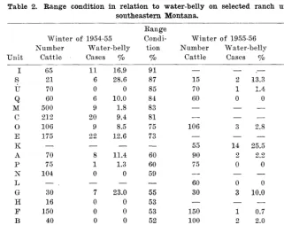
Range Condition and Water-belly
Incidence Table 2. Range coadition in relation to water-belly on selected ranch units in southeastern Montana.
Range condition on the units _
studied was predominantly good Winter of 1954-55 Condi- Range Winter of 1955-56 Condi- Range
(50 to 75% ) condition (Dykster- Number Water-belly tion Number Water-belly tion
huis, 1949). Sixteen units had Ullit Cattle Cases % % Cattle Cases % %
range in the good condition class, - T CK 11 -
nine units had range in the ex- cellent condition class, and only two units had range in the fair condition class. One unit was found to be on the line between good and excellent range condition.’ No units could be found where steers were carried through the fall and winter months on range that was in poor condition. Table 2 shows data on range condition and the incidence of water-belly on the ranches studied.
The water-belly incidence was slightly lower among cattle win- tering on good condition range than on excellent condition range. There were a total of 61 cases of
Eii
“021
U 70
Q 60
M 500
C 212
0 106
E 175
K -
A 70
P 75
N 104
L -,
G 30
H 16
F 150
B 40
D 90
V 48
II
6 0 6 9 20 9 22 -
8 1 0 -
Total 1,832” 100
16.9 91 - - .- -
28.6 87 15 2 13.3 87
0 85 70 1 1.4 85
10.0 84 60 0 0 84
1.8 83 - - - -
9.4 81 - - - -
8.5 75 106 3 2.8 75
12.6 73 - - - -
- - 55 14 25.5 66
11.4 60 90 2 2.2 60
1.3 60 75 0 0 60
0 59 - - - -
- - 60 0 0 57
23.0 55 30 3 10.0 55
0 53 - - - -
0 53 150 1 0.7 53
0 52 100 2 2.0 52
1.1 51 - - - -
0 28 48 0 0 28
4.37 - 859” 28 3.26 -
108 KARL G. PARKER Table 3. Incidence of water-belly in the winters of 1954-55 and 1955-56 on
selected southeastern Montana ranch= by range sites.
Site and Site, Complexes Overflow
Thin breaks, clayey and overflow
Saline upland and clayey Clayey
Clayey and saline lowland Savannah
Clayey (predominantly) and
overflow
Clayey, Savannah and overflow
No. Ranch Water- Water-
Unita belly belly
On Which Number Number Percent
Site Occurs Cases Cattle Incidence
1 0 98 0
1 0 16 0
1 0 110 0
11 126 3,469 3.34
1 5 144 3.47
3 16 398 4.07
2 11 235 4.66
1 24 345 6.96
water-belly was common. (See Table 3.)
Sites which supported a rather homogeneous cover mostly of grass- es or grasses and trees, to the ex- clusion of palatable shrubs and forbs, showed a higher incidence of water-belly during the study pe- riod of two years.
Cropland sites were not sur- veyed in detail, but it was observed that the incidence of water-belly in cattle on diversified cropland was very low compared to cattle on Savannah and clayey sites.
Yearly and Seasonal Incidence of Water-belly
During the two winters of this study, a record was kept of the chronological incidence of water- belly. The data obtained were graphed by semi-monthly periods -1st to 15th and 16th to the last day of month (Figure 2.).
There were 2,350 head of cattle included in this record during the winter of 1954-55 and 3,140 head of cattle during the winter of 1955- 56. One hundred thirty-two ‘cases, or a 5.62 percent incidence oc- curred in the 2,350 cattle, while only 44 cases, or 1.40 percent inci- dence occurred in the 3,140 cattle in the winter of 1954-55. This dif- ference presents a remarkable con- trast between the two years.
There is also a remarkable con- trast in the time of occurrence and the seriousness of the water-belly problem during the two winters
(Figure 2. ) . Weather appears to have been a definite influence.
It is well known to the residents, and particularly to stockmen in the study area, that the winter of 1955-56 was much more severe than the winter of 1954-55. United States Weather Bureau records (1956) bear this out. This suggests consideration of two outstanding factors (1) water, and (2) feed, as affected by snow cover.
Colder weather is known to cause reduced intake of water by cattle (Winchester and Morris,
1950). Reduced intake of water has been associated with increased incidence of water-belly by many ranchers. Data obtained through this project is definitely contra- dictory to such a theory. Less water-belly occurred during the colder of the two winters when cattle supposedly drank less water. The snow cover had a marked effect on the kind of feed available to cattle during these two winters. During the period November to January of the winter of 1954-55, snowfall was light. Most cattle grazed out on range and even were able to graze “short grasses”. There was wide-spread selective grazing on threadleaf sedge by cattle dur- ing this winter. Mild weather re- duced the normal supplemental feed requirement for this period. The feed situation was quite dif- ferent during 1955-56. A general snow fell on the range in the study area during the early part of No- vember. “Heavy feeding was nec- essary following the cold wave of the 11th (November 1955) and
WINTER OF
30
25
20
I5
IO
5
.O
SfCT p-CT6
ov.
YJ I5 - 16- 30
DEC. J A N. FE0 MAR APR.
30 I5 3; I- I5 16- 31 I- I5 I6- 31 I- I5 16. 29 I- I5 I6- 31 I- 15 I6- 30 FIGU~ 2. Yearly and seasonal incidence of water-belly in cattle on ranches studied
WATER-BELLY IN STEERS IN RELATION TO RANGE 109
was continuous through the 30th”. (U. S. Weather Bureau, 1956.) Many of the cattle were moved into ranch headquarters and given a maintenance feeding of supple- mental forage. During the rest of this winter there was very little grazing on the shorter range spe- cies until about March 1, 1956. Most ranches had an abundant supply of supplemental forage, much of which was alfalfa or mix- tures of alfalfa and grass hay, so there was more feeding than nor- mal.
This fortunate combination of weather and resultant management practices furnishes evidence which s t r 0 n g 1 y supports conclusions reached in other parts of this study-that grazing on mature, weathered grass is likely to cause water-belly in cattle. The “short grasses” appear to be more closely associated with the disease than the medium height species.
Water-belly in Relation to Minerals of Forage and Stock Water Samples
Chemical analysis of the samples of mixed range forage taken from the various ranches in this study were analyzed for phosphorus, cal- cium, magnesium, potassium, pro- tein, and silica. These data are re- ported on a moisture-free basis.
There was a highly significant negative correlation between the amount of phosphorus, calcium, magnesium, and potassium in the forage and the incidence of water- belly. There was a highly signif- icant positive correlation between the amount of silica in the samples and the incidence of water-belly in the steers. Table 4 shows the cod efficients of correlation.
Water used by the cattle con- tained very little calcium, phos- phorus, and silica. The contribu- tions of these minerals to the graz- ing animals’ diets from stock wa- ter was very small compared to that furnished by range and other forages. A steer would need to drink 1,000 gallons of water to acquire as much silica in its diet as it would get in one day from 30 pounds of range grass forage. The
Table 4. The incidence of water-belly in relation to planti minerals: coeficients of correlation.1
Incidence Incidence Incidence Incidence Incidence
Linear
V9. vs. vs. vs. vs.
Phosphorus Calcium Magnesium Potassium Silica
-5546”” -.4899”* -.5657*” --.4769** .5581**
**Significant at .Ol level
1 Statistical analysis was conducted by Montana State College Statistical Laboratory
mineral content of water is not considered to be an important fac- tor in the water-belly problem.
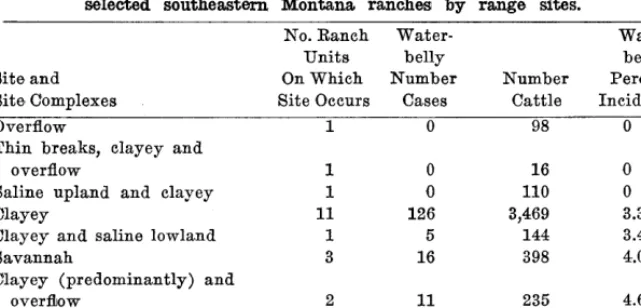
The corollary study of mineral content of western wheatgrass, green needlegrass, bluebunch wheatgr!ass, needle-and-t hr e ad, Junegrass, Sandberg bluegrass, blue grama, and threadleaf sedge revealed some new and valuable information.
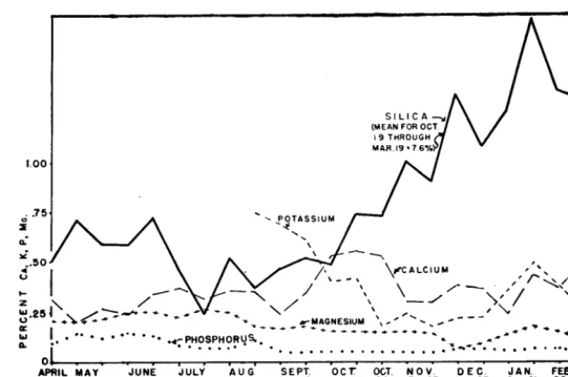
The trend in the mineral con- tent of these species during the year varied seasonally and in a way which again suggests relation- ships to the water-belly problem. The silica content of all plants was high during the late fall and win- ter-the season of high water-belly incidence. The content of potas- sium, phosphorus, and magnesium particularly, was low during that same season. Calcium followed a somewhat modified path, but was high during the early part of the water-belly season.
The silica was by far the most
abundant mineral found in the species sampled. Potassium ranked second to silica, followed by cal- cium, magnesium, and phosporus. These findings agree with those of Tobiska, et al., (1937), except that in their study, phosphorus ex- ceeded the magnesium. The trend in silica content by growth stages was similar to that found in an- nual plants in California ranges during the growing season, as re- ported by Gordon and Sampson
(1939).
The November 13 samples were divided and half of each sample was washed to determine the amount of superficial (soil) silica burden. Washing reduced the silica in the samples about one- twentieth. The residue washed from the samples contained 48 per- cent silica.
Figure 3 shows the mineral con- tent of the seven grasses and one sedge sampled by growth stages for one year.
1-v 3. i
/ -_ -.
/ . k!
,‘*POTASSIUM ’ . . ,
/ \ \ .2
\
ol 1
%Y
RAPID SHOOTING BLOSSOM SEED SEEDS SEED FALL SLIGHTLY MOSTLY EXT&ELY GROWTH g;LOL;$R RIPE DRY SOME SHATTER RE-CAST
WEATHEREDWEADTHER- WigtiER- GROWTH
FIQURE 3. Minerals in seven grasses and one sedge, by growth stages for one year : western wheatgrass, bluebunch wheatgrass, blue grama, threadleaf sedge, Junegrass, Sandberg bluegrass, needle-and-thread, and green needlegrass. Samples collected
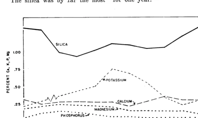
110 KARL G. PARKER Figure 4 shows the mineral con-
tent of the two “short grasses”, blue grama and threadleaf sedge, for one year (1954-55). The silica content of these two species was extremely high during the late fall and winter season, when there was a high incidence of water-belly in range cattle. The silica content of the important mid-grasses, western wheatgrass, needle-and-thread, and green needlegrass was lower and the content during the winter time was only 4.1 percent as compared to 7.6 percent for the so-called “short grasses.”
More recent research work along this line by the Montana Agricul- tural Experiment Station indicates that range shrubs such as saltbush, winterfat, greasewood, silver sage- brush, and rabbitbrush have a very low content of silica at all times, usually less than one percent.
APRIL MAY JUNE JULY AUG SEPT OCT OCT. N 0 V
24 IO 23 7 16 7 20 3 20 2 I7 I 15 29 13 27 II 2o 1964
FIGURE 4. Minerals in two “short grasses”-blue grama and threadleaf sedge-for one year, 1954-55. Sampled near Ashland, Montana.
From these results, it appears that the practical cattlemen can avoid some of the losses due to water-belly by remoping steers from native grass ranges as they dry up and moving the animals to range containing an abundance of palatable shrubs, legumes or green, immature grasses. Since many range areas, particularly in the Great Plains, have very little shrubby vegetation, planting fall pastures to grasses and legumes may offer some relief. Use of leg- umes and early cut grass hays to supplement range forage may also help reduce the incidence of this disease among steers on ranches where it is a problem.
and the mineral content of range forages and stock water in relation to the seasonal incidence of water- belly were investigated.
Studies were made of twenty- five ranches in the southeastern one-fourth of Montana which lies in the 10 to 14 inch rainfall belt. Most of the area is considered to be within the mixed prairie asso- ciation of the grassland formation. Comparable ranch units were stud- ied in pairs.
There was less water-belly in steers on range containing palat- able shrubs than on range contain- ing only grasses, or grasses and un- palatable shrubs.
)Summar y
Urolithiasis, or water-belly, is one of the greatest nutritional dis- ease problems of the beef cattle industry.
On ranches studied there were fewer cases per hundred steers of water-belly on good condition range than on excellent condition range.
This exploratory study was con- ducted for the purpose of develop- ing a better understanding of the rangeland factors which affect water-belly, and to find a means of reducing losses due to water- belly of range steers. The relation- ships of range vegetational types, range condition and range sites,
Where overflow and saline up- land sites were grazed independent- ly of clayey and Savannah sites, there was less water-belly.
The study of minerals in range forages and supplemental forages showed a strong positive correlation between silica content and water- belly incidence. The correlation was negative in the case of other minerals studied.
During the two years of this
a
w
0
.6
study, the seasonal incidence of water-belly in range cattle varied markedly. The difference in sea- sonal incidence in the two years and the difference in percentage in- cidence was attributed to a differ- ence in availability of weathered range forage due to snow cover. It is believed that reduced intake of weathered range grasses, particu- larly blue grama and threadleaf sedge, because of heavy snow cover, and the consequent increase in the feeding of good quality hay, played a part in reducing the incidence of water-belly during the winter of 1955-56 compared to the previous winter.
WATER-BELLY IN STEER8 IN RELATION TO RANGE 111
phosphorus were higher in the sum- mer and lower in the winter.
It is suggested that cattlemen can prevent some of the losses due to water-belly by making greater use of green fall pastures and leg- umes, by saving range with palat- able shrubs for fall and winter pas- ture for steer calves, and by feeding legume and early cut hays to steers prior to and during the normal water-belly season.
LITERATURE CITED
BYXKS, HORACE G., M. S. ANDERSON and RICHARD BRADFIELD. 1938. Genera.1 chemistry of soil. Soils and Men. U. S. Dept. of Agr. Yearbook of Agr. 1938: 911-928.
DYKSTEBHUIS, E. J. 1949. Condition and management. of grassland based
on quantitative ecology. Jour. Range Mangt. 2: 104-115.
ENSMINGER, M. E., M. W. GAL&AN and W. L. S~ocunf. 1955. Problems of the American cattleman. Wash. Agr. Exp. Sta. Bull. 562. 89 pp.
FORBES, E. B. and F. M. BEEIGLE. 1916. The minera, metabolism of the milch cow. Ohio Agr. Exp. Sta. Bull. 295. 26 pp.
GOKDON, AARON and A. W. SAMPSON. 1939. Composition of common Cali- fornia foothills plants as a factor in range management. Cnlif. Agr. Exp. St:\. Bull. 627. 95 pp.
JONES, J. M., W. H. BL~ICK, N. R. ELLIS and F. E. KEATING. 1949. The influ- ence of calcium and phosphorus sup- plements in sorghum rations for fat- tening steer calves. Texas Agr. Expt. Sta. Prog. Rept. 1190. Cattle Series 79.
MAIZXX, LOUIS L. 1954. TJnpublished
The Variable Plot Method for Estimating
Shrub Density
CHARLES F. COOPER
Depaatment of Bota.ny, Duke University, Durham, North Carolina!
Reliable measurements of shrub density on range lands can be made without the use of time-con- suming line transect or plot meth- ods. A quick, one-man system of counting shrubs can be used to es-’ timate the percentage of an area covered by woody plants. This procedure has been employed suc- cessfully to estimate densities of shrubs and half-shrubs ranging from 6 inches to 30 feet in crown diameter.
Usually called the variable-plot method, the system was developed 1 At the time that this article was pre- payed the author was employed by the Arizona Watershed Program, Phoenix,
Arizona.
in Austria. It was first proposed by Bitterlich (1948), who used it to make timber volume estimates without the necessity of establish- ing sample plot boundaries. Bitter- lich’s method was introduced to American foresters by Grosen- baugh (1952). A simple modifica- tion of the original technique per- mits it to be used to estimate shrub cover directly in percent.
progress report. Bgr. Res. Service. U. S. Dept. Agr.
MATHARCS, R. H. and A. K. SUTHERLAND. 1951. Siliceous renal calculi in cattle. Australian Vet. Jour. 27: 68-69.
SWINGLE, KAI& F. 1953. Chemical com- position of urinary calculi from range steers. Amer. Jour. Vet. Med. 14: 493-498.
TOEISKA, J. W., et al. 1937. Nutritional characteristics of some mountain meadow hay plants of Colorado. Colo. Agr. Exp. Sta. Tech. Bull. 21. 23 pp.
U. S. DEPT. OF COMIXERCE. 1954. Cli- matological data. Montana. Annual Summary. 57 (13).
U. S. DEPT OF COMRIERCE. 1955. Cli- matological data,. Montana. Annual Summary. 58 (13).
WINCHESTEE, C. F. and M. J. MORRIS. 1956. Water intake rates of cattle. Jour. Anim. Sci. 15: 722-740.
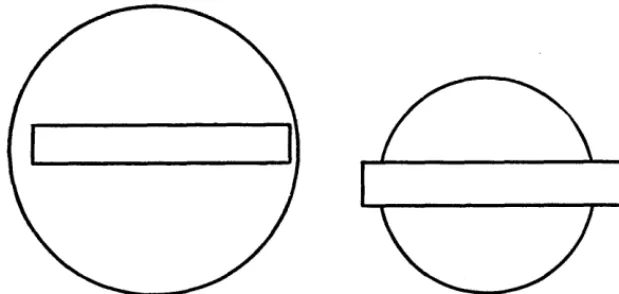
The variable-plot method re- quires no actual measurements in the field. No plots or lines are laid out on the ground, and it is un- necessary to measure the dimen- sions of any plant. The usual measured plots or lines are re- placed by a series of sampling points distributed at random throughout the area to be surveyed. At each sampling point, the ob- server views through the eyepiece of a hand-held angle gauge every shrub visible from that point. The angle gauge is illustrated in Fig- ure 1. Those shrubs are counted whose horizontal crown spread ap- pears larger than the crossarm of the angle gauge. Shrubs whose crown spread appears less than the length of the crossarm are ignored. Figure 2 is a schematic diagram showing a shrub that would be counted and one that would not. The distance at which a shrub is
WATER-BELLY IN STEER8 IN RELATION TO RANGE 111
phosphorus were higher in the sum- mer and lower in the winter.
It is suggested that cattlemen can prevent some of the losses due to water-belly by making greater use of green fall pastures and leg- umes, by saving range with palat- able shrubs for fall and winter pas- ture for steer calves, and by feeding legume and early cut hays to steers prior to and during the normal water-belly season.
LITERATURE CITED
BYXKS, HORACE G., M. S. ANDERSON and RICHARD BRADFIELD. 1938. Genera.1 chemistry of soil. Soils and Men. U. S. Dept. of Agr. Yearbook of Agr. 1938: 911-928.
DYKSTEBHUIS, E. J. 1949. Condition and management. of grassland based
on quantitative ecology. Jour. Range Mangt. 2: 104-115.
ENSMINGER, M. E., M. W. GAL&AN and W. L. S~ocunf. 1955. Problems of the American cattleman. Wash. Agr. Exp. Sta. Bull. 562. 89 pp.
FORBES, E. B. and F. M. BEEIGLE. 1916. The minera, metabolism of the milch cow. Ohio Agr. Exp. Sta. Bull. 295. 26 pp.
GOKDON, AARON and A. W. SAMPSON. 1939. Composition of common Cali- fornia foothills plants as a factor in range management. Cnlif. Agr. Exp. St:\. Bull. 627. 95 pp.
JONES, J. M., W. H. BL~ICK, N. R. ELLIS and F. E. KEATING. 1949. The influ- ence of calcium and phosphorus sup- plements in sorghum rations for fat- tening steer calves. Texas Agr. Expt. Sta. Prog. Rept. 1190. Cattle Series 79.
MAIZXX, LOUIS L. 1954. TJnpublished
The Variable Plot Method for Estimating
Shrub Density
CHARLES F. COOPER
Depaatment of Bota.ny, Duke University, Durham, North Carolina!
Reliable measurements of shrub density on range lands can be made without the use of time-con- suming line transect or plot meth- ods. A quick, one-man system of counting shrubs can be used to es-’ timate the percentage of an area covered by woody plants. This procedure has been employed suc- cessfully to estimate densities of shrubs and half-shrubs ranging from 6 inches to 30 feet in crown diameter.
Usually called the variable-plot method, the system was developed 1 At the time that this article was pre- payed the author was employed by the Arizona Watershed Program, Phoenix,
Arizona.
in Austria. It was first proposed by Bitterlich (1948), who used it to make timber volume estimates without the necessity of establish- ing sample plot boundaries. Bitter- lich’s method was introduced to American foresters by Grosen- baugh (1952). A simple modifica- tion of the original technique per- mits it to be used to estimate shrub cover directly in percent.
progress report. Bgr. Res. Service. U. S. Dept. Agr.
MATHARCS, R. H. and A. K. SUTHERLAND. 1951. Siliceous renal calculi in cattle. Australian Vet. Jour. 27: 68-69.
SWINGLE, KAI& F. 1953. Chemical com- position of urinary calculi from range steers. Amer. Jour. Vet. Med. 14: 493-498.
TOEISKA, J. W., et al. 1937. Nutritional characteristics of some mountain meadow hay plants of Colorado. Colo. Agr. Exp. Sta. Tech. Bull. 21. 23 pp.
U. S. DEPT. OF COMIXERCE. 1954. Cli- matological data. Montana. Annual Summary. 57 (13).
U. S. DEPT OF COMRIERCE. 1955. Cli- matological data,. Montana. Annual Summary. 58 (13).
WINCHESTEE, C. F. and M. J. MORRIS. 1956. Water intake rates of cattle. Jour. Anim. Sci. 15: 722-740.
The variable-plot method re- quires no actual measurements in the field. No plots or lines are laid out on the ground, and it is un- necessary to measure the dimen- sions of any plant. The usual measured plots or lines are re- placed by a series of sampling points distributed at random throughout the area to be surveyed. At each sampling point, the ob- server views through the eyepiece of a hand-held angle gauge every shrub visible from that point. The angle gauge is illustrated in Fig- ure 1. Those shrubs are counted whose horizontal crown spread ap- pears larger than the crossarm of the angle gauge. Shrubs whose crown spread appears less than the length of the crossarm are ignored. Figure 2 is a schematic diagram showing a shrub that would be counted and one that would not. The distance at which a shrub is
CHARLES F. COOPER
FIGURE 2. Schematic dkgram of two shrubs viewed with the angle gauge. The shrub on the left would be counted; the one on the right would not.
counted depends upon its size. Large shrubs are counted at a greater distance from the observer than small ones.
To determine shrub crown den- sity in percent, it is necessary only to divide the average shrub count for all the sampling points by a s predetermined constant. This con- stant is determined by the dimen- sions of the angle gauge. The num- ber of sampling points required on any area depends on the desired intensity of the survey.
Principle of the Methold The plots from which the method takes its name are entirely the- oretical-they are not laid out on the ground. Each sampling point is the center .of several theoretical circular plots of varying radii
(Husch, 1956). At each sampling point, there are many overlapping plots with a common center, each plot corresponding to one of the shrubs counted with the angle gauge.
Let us assume that an angle gauge has an overall length of 30 inches, with a crossarm six inches long. When held to the eye, this gauge intercepts a horizontal angle of 9’25’. This angle just includes a circle at five times its diameter from the observer. A circle that intercepts a larger angle than 9 “25’ will appear larger than the instrument crossarm, and is closer to the eye than five times its diame: ter. One which intercepts a smaller
angle is farther away and will ap- pear smaller than the cross arm. These relations follow from the fact that the overall length of the gauge is five times the length of its crossarm.
A small circle occupies one per- cent of the area of a large circle if the radius of the large circle is five times the diameter of the small one. For instance, a circle ten feet in diameter has an area of about 78.54 square feet. A large circle whose radius is five times the di- ameter of the small one, or fifty feet, has an area of 7,854 square feet. Thus, the small circle occu- pies one percent of the area of the large one.
Now let us consider a shrub stand as observed with the angle gauge from a single sampling point. Any shrub whose horizontal crown spread appears exactly equal to the length of the crossarm is five times its own diameter from the sampling point; if it appears to extend beyond the edges of the crossarm it is closer than this limit. These are the shrubs that are counted.
Each shrub counted with the angle gauge occupies one percent of the area of a hypothetical plot whose radius is five times the di- ameter of the shrub. When a shrub is observed with the angle gauge, a theoretical plot of this radius is automatically set up. The limits of this plot are established by the fact that if a shrub is outside the plot, it appears smaller than the
instrument crossarm and is not counted. Each shrub counted therefore represents one percent shrub cover, and the total number counted is the percent of shrub cover at that sampling point.
A numerical example may help make this clear. A shrub, exactly ten feet in diameter, is located 25 feet from a sampling point. When this plant is observed through the angle gauge, a theoretical plot fifty feet in radius is automatically set up, and the shrub is observed to lie within this plot. Since the area of the shrub is 78.54 square feet, and that of the plot is 7,854 square feet, the shrub occupies one percent of the theoretical plot. At first glance, it might appear that since this shrub is less than fifty feet from the plot center, it repre- sents more than one percent ground cover. A little thought will show that this is not so. The angle gauge sets up a maximum limit beyond which shrubs are not counted, and any shrub within this limit represents one percent of the area of the hypothetical plot.
A second shrub ten feet in di- ameter forty feet from the observ- er is still within the fifty foot limit, and it also occupies one percent of the area of the plot. If these two are the only shrubs which lie within five times their own di- ameter from the plot center, the shrub density at that sampling point is two percent, no matter how many plants there may be on the area that are more than five times their diameter away. If, however, a shrub twenty feet in di- ameter is sixty feet from the ob- server, it also is less than five times its diameter away. Its theo- retical plot has a radius of 100 feet, and the shrub occupies one percent of the plot. These three plants taken together then indicate a three percent ground cover at that sampling point.
VARIABLE PLOT METHOD FOR SHRUB DENSITY 113
this limit represents the percent of ground cover at that point. Many other shrubs will be visible from each sampling point, but only those that lie within the specified limit contribute to the estimate of ground cover. The variable-plot method is nothing more than a means of counting all the shrubs that lie within this limit.
The instrument just described is unwieldy and hard to use in the field. Better results are obtained if the crossarm is made smaller, thus intercepting a smaller angle. A smaller crossarm means that shrubs will be counted at a greater distance from the eye, and that more than one shrub will be need- ed to equal one percent ground cover. Therefore, with a smaller crossarm the shrub count must be divided by a constant to determine the percent of shrub density.
To determine the relation be- tween this constant and the di- mensions of the instrument, it is necessary to consider the mathe- matics of the method. Percentage of ground cover may be written
n S2
P=- x 100 U-1
(2R) 2
where P is percentage, n is number of shrubs on the plot, S is shrub diameter in feet, and R is plot radius in feet. The angle gauge is so constructed that
W
S
-=-
(2)
IJ
Rwhen W is the length of the cross- arm and IJ is the overall length of the instrument (more precisely, the distance of the crossarm from the eye). Substituting in (l),
W2
P=nx- x 100 (3)
(2U2
This can be expressed in the form Il
w= (4)
n 5+---
P
If r is the constant by which the shrub count at any point must be divided to find the percentage of ground cover, then
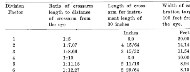
Table 1. Convenient division factors and crossarm lengths. Division
Factor
1 2 3 4 5 6
Ratio of crossarm lengt,h to distance of crossarm from the eye
1:5 1: 7.07 1: 8.66 1:lO 1: 11.18 1: 12.27
Length of CPOSS- Width of cali- arm for instru- bration targkt at ment length of 100 feet from
30 inches the eye.
Inches Feet
6.0 20.00
4 15/64 14.14
3 E/32 11.54
3.0 10.00
2 11/16 8.94
2 29/64 8.15
P = -? and r = -? (5) P Substituting ;5) in equation (4)) the final form becomes
IA
w=- (6)
5Vr
It should be pointed out that this formula is mathematically not strictly accurate. A correction should be made for the fact that the line of sight intercepts a chord closer to the observer than the true crown diameter. The error due to omission of. this correction is so small as to be almost unde- tectable in variable-plot sampling. From equation (6) it can be seen that if an instrument is 30 inches long and has a division con- stant of 2, its crossarm must be 4.24 inches long. The ratio of crossarm length to the distance of the crossarm from the eye is 1:7.07. Table 1 lists several other conveni- ent division constants, with their accompanying ratios and crossarm lengths.
Construction and Use of the
Instrument
The angle gauge can easily be made from a strip of hardwood and some scrap metal. Extruded aluminum angles of the “do-it- yourself” variety sold by hardware stores make excellent material for the eyepiece and crossarm. The angles should be about 11/4 inches on a side. The eyepiece should have a viewing hole about 3/s inch in diameter. An instrument length of about 30 inches is convenient. If it is much shorter, difficulty will be experienced in keeping both
the crossarm and the more distant shrubs in focus at the same time. To illustrate the procedure fol- lowed in using the variable plot method, Table 2 lists the actual counts from a field trial made in an open stand of creosote bush (Larrecc triderztata) and palo Verde ( Cercidiwn
micro
pit
yllwrn).
The angle gauge was calibrated to re- quire a division constant of 2. Twelve sampling points were lo- cated at arbitrary intervals of four chains, on two lines through the area. From each sampling point, those shrubs were counted whose diameters appeared larger than the crossarm. The counts were totaled and divided by 12 to find the average. This average was then divided by 2, the division constant of the instrument, to estimate the percentage of the area covered by shrubs. In this case, the totalTable 2. Sample variable-plot tally in a creosote bush type.
Shrubs Counted Sampling Creosote Pdo Verde
Point Bush
1 22 4
2 21 9
3 27 11
4 49 8
5 27 7
6 23 10
7 29 7
8 40 7
9 38 14
10 29 16
11 40 9
12 29 2
Total 374 104
Average 31.17 8.67
114
crown density of creosote bush was estimated at 15.6 percent; that of palo verde at 4.3 percent.
The principal difficulty in the use of the variable-plot method is that distant shrubs which should be counted tend to be obscured by those nearby. This difficulty is minimized by using a crossarm length which permits a division factor of 2. Shorter crossarms, with larger division constants, are occasionally useful in very sparse and open shrub stands. A longer crossarm, with a division constant of unity, becomes completely un- manageable, and introduces seri- ous errors.
In dense shrub stands, many dis- tant shrubs are obscured and ac- curacy falls off rapidly. The meth- od is not very reliable where den- sities exceed about 35 percent. For this reason, it is best suited to sparse desert-shrub types, to areas of shrub invasion in grasslands, and to other open types. Tf the plants are small, it is necessary to crouch down in order to keep the line of sight nearly horizontal.
Steep slopes require a correction of shrub counts to increase accur-
acy. The count at any point is
multiplied by the secant of the angle of slope perpendicular to the contour. An average slope correction can be used if shrub density does not change markedly with changes in slope.
Another possible source of trou- ble lies in the distance of the cross- arm from the eye. It is this dis- tance which determines the char- acteristics of the angle gauge, rather than the actual overall length of the instrument itself. It is best to use the following cali- bration procedure in adjusting the final position of the crossarm. Sup- port the instrument firmly and measure a distance of 100 feet from the eyepiece. At this distance, lay out a target at right angles to the line of sight. If the angle has a division constant of 2, the target should be 14.14 feet across. Sizes of target for other constants are listed in Table 1. With the eye- piece held firmly against the bones
(‘HARLKS F. COOPER
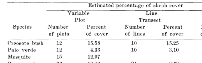
Table 3. Results of tests of variable-plot method in various shrub types. Estimated percentage of shrub cover
Variable Line 100%
Plot Transect Tally
Species Number Percent Number Percent Percent
of plots of cover of lines of cover of cover
Creosote bush 12 15.58 10 15.25
Palo Verde 12 4.33 10 3.10
Mesquite 15 12.07 12.64
Burroweed 36 10.43 24 9.i8
sllrrounding the eye, move the crossarm backward and forward on the wooden base until the target is exactly covered. Fasten the crossarm securely at this point. A slotted bolthole on the crossarm fa- cilitates calibration. If eyeglasses are worn, the instrument can be made shorter so that the eyepiece rests against the ,glasses.
The data obtained from vari- able-plot samples are subject to the usual statistical analyses. Com- monly used formulas can be used to compute standard deviation, standard error of the mean, and other useful statistics. Further- more, variable-plot data lend them- selves readily to the calculation of an index of dispersion. This index is a measure of the spatial distribu- tion of individual plants, indicat- ing whether they are more or less uniformly distributed than would be expected as a result of pure chance. Rice and Penfound (19%) describe in detail the method of calculating this illdex, whicll is of value in many ecological studies.
Bitterlich’s method was first used to measure basal area of tree stems in square feet per acre. For this purpose, a crossarm length to eye distance ratio of 1:33 has com- tionly been used, rather than the 1:7.07 recommended for shrubs. Estimates using this small cross- arm have been found quite reliable in forest stands (Rice and Pen- found, 1955 ; Shanks, 1954). Husch
(1955) found that he obtained more accurate estimates of basal area by usin, “a a 1:16.5 ratio. All of these investigators found that the variable-plot method took much less time than the conventional methods with which it was com- pared.
Cumparisons with Other Sampling Methods
Several tests were made to com- pare the variable-plot procedure with standard estimating methods in diverse shrub types in southern Arizona. Results of these compari- sons are summarized in Table 3.
Data were available on the per- centage of crown cover in a 6-acre stand of mesquite (Prosopsis jllli- florn). The crown area of each tree had previously been measured, and the percent of grqund cover de- termined. The complete tally showed a cover density of 12.64
percent, lvhile the variable-plot samples estimated density to be 12.07 percent.
The variable-plot method was next compared with the line tran- sect method (Canfield, 1941) in common use by range technicians. As the line transect method is gen- erally considered to give fairly re- liable estimates of plant density, a comparison of the two methods will presumably give an index to the accuracy of the variable-plot technique.
The 12 variable-plot samples in the creosote bush stand previously described were compared with aLen 200-foot line transects run through the same area. The variable-plot samples gave a creosote bush den- sity estimate of 15.58 percent, while the line transect estimate waq 15.25 percent. There was a greater difference in the palo *Verde estimates, which were 4.3 percent and 3.1 percent, respectively. How- ever, the palo verdes were so wide- ly scattered that neither sample was adequate.
VARIABLE PLOT METHOD FOR SHRUB DENSITY 115
variable-plot samples was taken from the same sample points as in the first survey, using an instru- ment with a division constant of 4. Collection of the data for this second set of samples took longer than the first because of the great- er number of shrubs that had to be counted, and to the greater effort required to avoid missing some. In spite of all precautions, a few were evidently missed, because the 4X angle gauge yielded a density esti- mate of only 14.3 percent for the creosote bush, compared with the previous estimate of 15.6 percent. The palo verde estimate was almost the same for the two instruments, because of the large size and small number of these trees, which were easily visible even at a distance.
A final comparison was made in a stand of burroweed (Happlopap- pus tenzhectus), a desert half- shrub averaging about one foot in diameter. Thirty-six variable-plot samples were compared with 24 line transects, each 100 ,feet long. The variable-plot density estimate was 10 43 percent, while that by line transects was 9.7 percent. The difference between these two* re- sults was less than the expected sampling error calculated for ei- ther method.
Since .lhese ‘tests compared one sampling method with another, it was not possible to calculate the statistical significance of the differ-
ence between them. IIowever, it has generally been considered that any sampling method is satisfac- tory that yields an estimate within 10 percent of the true cover den- sity. The agreement between the variable-plot estimates and those made ,by other methods strongly suggests that density estimates made by the variable-plot method will fall well within these limits.
The variable-plot technique is most applicable where nearly cir- cular objects are sampled. If shrub crowns are extremely irregular, considerable bias will be intro- duced. For this reason, the method is most useful in reconnaisance and extensive surveys. In forestry work, the angle prism suggested by Bruce (1955) has been widely adopted instead of a stick. This idea could be tried for estimating shrub cover, but the angle prism appears to have fewer advantages in counting ,shrubs than it does in counting small tree trunks.
Summary
The variable-plot method can be used to estimate shrub density in percent without measurement of distance or area. This method is faster and easier to apply than any of the standard shrub-estimating procedures now in common use. In tests in three different vegetation types, it closely approximated the
WALTER DUTTON, back from his F.A.O. range assignment in Argentina, is enthusiastic about the future pos- siblilities for increased livestock produc- tion in that country. Breeding stand- ards are high. A fa,vora.ble climate over much of the area allows exceptionally long growing periods. Grazing capaci- ties on both natural grasslands and artificial pa.stures are outstanding-in many places 2 to 5 acres per hea.d per cow for one year. Currently, however, the outlook is not encouraging. Gen-
Report On Argentina
era1 failure during the growing period to convert surplus fora,ge to hay and silage for use in winter is the main stumbling block to increased produc- tion. All too common are low calving and lambing percentages, long periods for steels to reach maturity, and heavy incidence of f{?ot-and-mouth disease, stemlning directly from lack of ade- quate feed during critical periods. On the other hand, and indicative of what can be done, a few outfits are rnarket- ing 18 month old steers, weighing 1100
estimates obtained by other sam- pling methods. It is most reliable in open shrub stands with a den- sity of less than 35 percent ; be- yond that point accuracy falls off rapidly. Variable-plot data are subject to statistical analysis, and are particularly useful in calculat- ing an index of dispersion. The variable-plot method appears to be a practical means of reducing the labor required in collecting field data on &rub density.
LITERATURE CITED
BITTEIILI~H, W. 1948. Die Winkelzahl- probe. Allgcmcine Forst-und-Holzwirt- schaftliche Zeitung. 59 (l/a) : 4-5. BRUCE, DAVID. 1955. A new way to look
at trees. Jour. Forestry 53 : 163-167.
CANFIELD, R. W. 1941. Application of the line interception method in sam- pling range vegetation. Jour. Forestry :<9 : 388-394.
GKOSENHAUGII, L. R. 19.52. Plotless tim- ber estimates-new, fast, easy. Jour. Forestry. 50: 32-37.
H~SCII, B. 19,X. Results of an inrestiga- tion of the variable plot method of cruising. Jour. Forestry. 53 : 570-574. -. 1956. Comments on the variable plot method of cruising. Jour. Forestry.
54: 41.
RICE, E. L. and W. T. PENFOUXD. 1955. An evaluation of the variable-radius and paired-tree methods in the black- jack-post oak forest. Ecology. 36: 335- 320.
SHANKS, R. E. 1954. Plotless sampling trials in Appalachian forest types. Ecology 35 : 237-244.
Differential Effect
on Range Species
of Herbage Removal
HORTON M. LAUDE, AMRAM KADISH, AND R. MER- TON LOVE
Associate Professor, Graduate Stu,dent, aw-$ Professor of Agrolzomy, Departme& of Agros&orny, Urt,iversity of Cal& f orwia, Davis, Calif or&u.
An extensive survey of Cali- fornia livestock operations con- ducted over nearly a decade by Jones and Love (1945), revealed that the various ranges exemplified every degree of transition from better species toward poorer and vice versa.
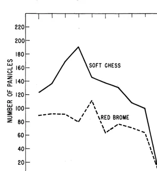
In every case the trend upward or downward in grazing values was a direct result of practices applied. Where livestock were grazed on a given range only while the plants were green and growing, and were removed before soil ‘moisture be- came inadequate for maturing the better annuals and perennials, the transition toward better feed pro- ceeded rapidly, provided the live- stock load was neither excessive nor too light. On the other hand, where livestock use was deferred until the more rapidly developing annuals had reached the flowering stage or later, the transition to- ward poorer quality feed was rapid. When a range was used on a year-long basis, the transition to poorer feed was somewhat slower, but range deterioration was in progress as evidenced by an in- creasing population of weedy plants. Even low rates of stocking did not answer this last problem, because this allowed more oppor- tunity for selective grazing. Such was evidenced by the development of larger and larger colonies of undesirable species that early be- came unpalatable, e.g. red brome (Bromus rub ens ) , annual fescues (PestzLca spp.), annual foxtail bar- leys (Hordeurn spp.), and ripgut
(Bromus rigidus). This was ac-
companied by a decrease in the
population of desirable annuals such as bur clover (Medicago his- pida) and soft chess (Bromus mol- Zis).
Grazing Treatment
These observations indicated strongly that range species react differentially to grazing treatment. Love (1944, 1952) reported the re- sults of experiments showing high- ly significant response of perennial grasses to early and deferred graz- ing, especially with respect to stand establishment of the peren- nials. For instance, line transect counts of seeded Stipa pulchra showed 111 plants following early grazing, while only 23 plants were counted under deferred grazing. With S. cernua the plant counts following the two grazing treat- ments were 228 and 24, respec- tively. Depending on the grazing treatment, Love and Williams (1956) reported significant differ- ences in bur production of Medi- cage hispida. Continuous grazing throughout the season was com- pared with a grazed-ungrazed- grazed treatment. The latter re- sulted in 2,264 pounds of burs per acre left on the ground at the end of the season compared with only 664 pounds in the continuously grazed field. These investigators suggested that alternating the two treatments annually would prob- ably result in a high level of an- nual bur production as well as lamb gains.
Growl& Ctiracteristics
Manipulation of species on the range can be guided by critical study of the growth characteris-
116
tics of the individual plants, Bran- son (1953) reported differences in growth habit in perennial grasses in regard to elevation of the grow- ing points and the ratio of flower stalks to vegetative stems, and re- lated these characteristics to the tendency of the grasses to decrease or increase under grazing.
Differential responses to herbage removal among species should be recognized so they may be utilized to advantage through proper graz- ing management. In annual grass- es especially, the production of tillers, heads, and seed relate to persistence under grazing. The in- vestigation of such features, par- ticularly as affected by the timing of herbage removal, was the objec- tive of the following studies.
November plantings of soft chess (Bromus mollis), foxtail fescue (Pestuca megalura) , slender wild oats (Avena barbata), and Medi- terranean barley (Hordeum hys- trix) were made in replicated 4- foot rows in the field at Davis for two years to compare the effect on growth termination of clipping the spring following planting. Clip- ping was at 3 to 4-inch height, commencing when the “early boot” stage was reached. Such clipping removed the immature inflorescence of the elongating culm, thereby stimulating the development of tillers. By repeating the clipping at approximately two-week inter- vals, the growing points of succes- sive sets of tillers were removed, and vegetative growth through the production of new tillers was stim- ulated. The tillers became pro- gressively shorter and fewer, how- ever, as the season advanced.
EFFECT OF HERBAGE REMOVAL ON RANGE SPECIES 117
It should be observed that these re- sponses were obtained on deep and fertile soil, with reduced competi- tion from other species, and in a season of favorable rainfall distri- bution through February, March, and April. The last effective rain fell April 27-28 and totaled 1.3 inches.
heads, and each successive rank of heads tended to be slightly shorter than the preceding ones.
Greenhouse Study
Foxtail fescue differed from soft chess in that, following the second clipping, growth was reduced markedly and essentially was ter- minated after the third herbage re- moval. Such behavior agrees with the very early maturity exhibited by this species in the field.
nounced effect on the behavior of a species, very little quantitative data are available on these re- sponses. A field seeding was in- tensively studied to determine the effects of timing of herbage re- moval on regrowth and culm de- velopment, seed characteristics, and growth cessation in two species of annual grass ; namely, soft chess and red brome.
To study individual plant be- havior more thoroughly, green- house plantings of soft chess and of foxtail fescue were made pe- riodically in 6-inch pots. Plants were thinned to three per pot, and 27 plants comprised a treatment. Growth conditions were maintained to permit development to maturity regardless of the date of planting, this being accomplished in winter by providing long photoperiods.
Field Clipping
Unlike plants in the greenhouse, those in the field are subjected to variation in environment and re- spond with seasonal growth. Here the effects of herbage removal have importance in regard to the regu- lation of growth from the stand- point of grazing management.
Clippings were made at 11/2 inch height, when the first heads were emerged. Measurements included dry weights of clipped tissue, head height, and tillering behavior. Two clipping procedures were employed in each planting. One treatment was clipped twice, giving oppor- tunity to compare the first re- growth with the original produc- tion. The other was clipped re- peatedly as each successive rank of tillers headed, and indicated the potential growth duration.
Though it is well-known that the time of herbage removal has a pro-
The two species were seeded on November 19, 1954, at a depth of l$$ inches in 5foot rows spaced 12 inches apart. Treatments were randomized with four replications. Eleven inches of rain fell between planting and May 8, this latter date marking the last effective rain of the season. With the exception of a dry March, the distribution pattern of the precipitation was relatively normal. Growing condi- tions were favorable, though cool-
,
I
I
I I II
I I I I220-
200-
Under the conditions of this experiment soft chess continued growth by repeated tillering and heading over a prolonged period. A mid-March planting was still tillering and heading in April of the following year. By then it had been clipped eight times, and twp- thirds of the plants had died. However, there had been 83 per- cent survival through the fifth clip- ping.
180-
2
= 160-
z
3 140~-
k5 120-
a
g IOO-
= 80-
60-
Certain comparisons between the original growth and subsequent re- growth of soft chess were noted under these greenhouse conditions. The dry weight per plant of both the first and subsequent regrowth was approximately one-fifth that of the first production. The average head height of the first regrowth was 40 percent that of the original