Detection and Modeling of Non-Gaussian Apparent
Diffusion Coefficient Profiles in Human Brain Data
D.C. Alexander,
1*
G.J. Barker,
2and S.R. Arridge
1This work details the observation of non-Gaussian apparent diffusion coefficient (ADC) profiles in multi-direction, diffusion-weighted MR data acquired with easily achievable imaging pa-rameters (b⬇1000 s/mm2). A technique is described for mod-eling the profile of the ADC over the sphere, which can capture non-Gaussian effects that can occur at, for example, intersec-tions of different tissue types or white matter fiber tracts. When these effects are significant, the common diffusion tensor model is inappropriate, since it is based on the assumption of a simple underlying diffusion process, which can be described by a Gaussian probability density function. A sequence of models of increasing complexity is obtained by truncating the spherical harmonic (SH) expansion of the ADC measurements at several orders. Further, a method is described for selection of the most appropriate of these models, in order to describe the data adequately but without overfitting. The combined procedure is used to classify the profile at each voxel as isotropic, anisotro-pic Gaussian, or non-Gaussian, each with reference to the un-derlying probability density function of displacement of water molecules. We use it to show that non-Gaussian profiles arise consistently in various regions of the human brain where com-plex tissue structure is known to exist, and can be observed in data typical of clinical scanners. The performance of the pro-cedure developed is characterized using synthetic data in order to demonstrate that the observed effects are genuine. This characterization validates the use of our method as an indicator of pathology that affects tissue structure, which will tend to reduce the complexity of the selected model. Magn Reson Med 48:331–340, 2002.©2002 Wiley-Liss, Inc.
Key words: diffusion tensor magnetic resonance imaging; hu-man brain; non-Gaussian; spherical harmonic; model selection
Diffusion imaging, particularly diffusion tensor magnetic resonance imaging (DT-MRI) (1) has become popular be-cause of the insight it provides into the structural connec-tivity of tissue (2,3). Water is a large constituent of biolog-ical tissue, and water molecules in tissue constantly un-dergo random, Brownian motion. Tissue also contains rigid structures, such as the walls of cells, that form bar-riers to diffusion, and it is this hindrance to diffusion that allows tissue structure to be probed through measure-ments of water mobility due to diffusion processes. In some types of tissue, such as most gray matter in the brain, the structure has no preferred orientation and so causes approximately the same amount of hindrance to diffusion
in all directions. The amount of diffusion or water mobil-ity is thus approximately equal in all directions, i.e., iso-tropic. Other types of tissue, however, have ordered struc-ture that hinders diffusion to different degrees in different directions, causing diffusion anisotropy. White matter in the brain, for example, consists of bundles of axon fibers, and water is free to diffuse along the axis of the fibers but is hindered in the perpendicular directions.
The diffusion of water molecules in tissue over some time interval,t, can be described by a probability density function, pt, on the displacement, x, of water molecules after time t.pt reflects the underlying tissue microstruc-ture, because it is largest in the directions of least hin-drance to diffusion and smaller in other directions. In white matter, for example, pt is largest in directions par-allel to fibers, but is small in perpendicular directions and thus reveals fiber orientations. The goal of diffusion imag-ing is to obtain information about pt that leads to mean-ingful inferences about the microstructure of the material being imaged.
ptcan be shown to relate to the NMR signal attenuation,
S(q), measured through a pulsed gradient spin-echo exper-iment, via a Fourier transform (FT) with respect to q
⫽
␥␦G kˆ(4,5):
S共q兲⫽
冕
pt共x兲exp(⫺iq䡠x)dx. [1]
The spin-echo attenuation, S(q
), is defined as the
nor-malized diffusion-weighted signal,s(q
)/s(0), wheres(q) is
the NMR signal in the presence of a diffusion-weighting gradient of magnitude Gand direction kˆ, and s(0) is the signal in the absence of any such gradient.␦is the length of the gradient pulse, and␥is the magneto-gyric ratio of protons in water. We note that Eq. [1] relies on the fact that ␦ is negligibly small compared to t. This assumption is rarely justified in practice, but the effect of non-negligible ␦ is merely to introduce a convolution over a range of diffusion times (6) into the measurements, which gener-ally preserves the large-scale structure and orientation of the inferredpt.
Given enough measurements ofS(q
) spread over a
suit-able range of q
, the FT can be inverted to obtain an
esti-mate of pt. A more common approach, however, is to assume a simple model for pt the FT of which can be related directly to the spin-echo attenuation, which allows
ptto be inferred from a much sparser set of measurements. The simplest model forptthat incorporates second-order statistics (anisotropy) is a multivariate, zero-mean Gauss-ian, which has covariance 2Dtat timet:
pt共x
兲⫽
1
冑
共4t兲3兩D兩exp冋
⫺x
TD⫺1x
4t
册
. [2]1Department of Computer Science, University College London, London, UK. 2Institute of Neurology, University College London, London, UK.
Grant sponsor: Multiple Sclerosis Society of Great Britain and Northern Ire-land.
*Correspondence to: Daniel Alexander, Dept. of Computer Science, Univer-sity College London, Gower Street, London WC1E 6BT, UK. E-mail: [email protected]
Received 27 July 2001; revised 7 March 2002; accepted 9 March 2002. DOI 10.1002/mrm.10209
Published online in Wiley InterScience (www.interscience.wiley.com).
This is the distribution of an initial point concentration atx⫽0,t⫽0, diffusing according to the simple anisotro-pic diffusion equation (7):
pt
t ⫽ⵜ共Dⵜpt兲. [3]
The FT ofptis then also Gaussian, which gives rise to a simple relationship between the parameters ofpt(the ele-ments ofD) and the spin-echo attenuation:
S共q
兲⫽exp关⫺tq
TDq
兴⫽exp关⫺bkˆ
TDkˆ
兴. [4]
In Eq. [4],bis the diffusion-weighting factor given by
b⫽t|q
|
2.
The simplest form of diffusion-weighted (DW) MRI (8) models pt with a Gaussian in one dimension. A single spin-echo attenuation measurement allows the single pa-rameter of pt—its scalar variance—to be estimated from Eq. [4]:
d共kˆ
兲⫽⫺
1
blogS共q兲. [5]
The diffusion coefficient, d(kˆ), is proportional to the variance of the Gaussian model, which describes the root mean squared displacement of water molecules in the direction of the applied DW gradient kˆ. In DW-MRI, the measure of d(kˆ) obtained from Eq. [5] is often called the
apparent diffusion coefficient (ADC) (1), both because it
represents a spatial average of the diffusion coefficient over an image voxel and because it is based on this Gauss-ian assumption, which may be unjustified.
DT-MRI extends this basic idea to 3D, where the diffu-sion coefficient is described by a diffudiffu-sion tensor (DT),D, which is proportional to the covariance matrix of the tri-variate Gaussian, as in Eq. [2].Drelates to the 1D diffusion coefficientd(kˆ) in any chosen directionkˆas follows:
d共kˆ
兲⫽kˆ
TDkˆ
. [6]
In 3D,Dis a symmetric 3⫻3 matrix and thus has six free parameters. A minimum of six estimates of d(kˆ) in independent directions is thus required to estimate D, which requires six measurements of the spin-echo attenu-ation (seven MR measurements in total) to be made with the DW gradient applied in these independent directions. The estimate of Dobtained from such a set of measure-ments is referred to as theapparentdiffusion tensor (ADT) (1), as in the case of the ADC.
We define the “ADC profile” to be the estimate ofd(kˆ) over the range ofkˆ, which is the unit sphere. Whenptis Gaussian, the ADC profile is described by Eq. [6], and a standard approach (9) to the estimation ofDis to acquire DW images in a large number of directions (many more than six) spread evenly over the unit hemisphere. This oversampling of the ADC profile provides a more robust estimate ofD. Note that the antipodal symmetry ofptand henced(kˆ) is assumed, so thatd(kˆ)⫽d(⫺kˆ) and only half of the sphere needs to be sampled. Whenptis not Gaussian
the ADC profile deviates from that described by Eq. [6], and this kind of multiple gradient direction scheme af-fords the possibility of observing significant deviations should they arise.
It has long been recognized (1,10 –14) that the Gaussian, DT model is inappropriate when complex tissue structure is found within a single image voxel. There are alternative models forptthat can capture certain non-Gaussian effects that occur in these circumstances. A simple alternative is the multi-Gaussian model (10,11). This model is based on the assumption that a voxel containsnseparate compart-ments, each containing a different tissue type in propor-tionai(⌺iai⫽1,i⫽1, . . .n) and that the diffusion within each compartment can be described by a Gaussianptwith DT, Di. The model assumes further that there is no ex-change of molecules between these separate compart-ments.ptthen becomes a weighted sum of Gaussians and Eq. [4] becomes:
S共q
兲⫽
冘
i⫽1 naiexp(⫺bkˆ
TD ikˆ
). [7]
With this model forpt, the ADC profile can have shape very different from that described by Eq. [6], which is often modeled poorly by a single DT (10). Figure 1 shows ADC profiles simulated from prolate, oblate, and isotropic Gaussian pt’s, together with profiles obtained from bi-Gaussian pt’s that combine them. Note the characteristic peanut shape of the prolate Gaussian ADC profiles and the “filled bagel” or red blood cell shape of the oblate Gaussian profile, which are typical of Gaussian functions plotted over a sphere. The contours of the corresponding Gaussian functions in 3D have the more familiar ellipsoidal con-tours: cigar-shaped in the prolate case, and Frisbee-shaped in the oblate case.
Alexander et al. (10) analyzed the behavior of the ADC profile within voxels containing multiple tissue compart-ments. They showed how the observability of higher-order profiles increases (their non-Gaussian shape becomes more pronounced) with the size of the diffusion-weighting factor, b. They used the instability of the DT and its de-rived scalar measures, such as the mean diffusivity and fractional anisotropy, to locate regions in the brain where the DT description of the ADC profile is poor. Several regions in data acquired withb⫽3000 s/mm2were high-lighted by this approach, including the pons, corpus cal-losum, cingulum, internal capsule, and arcuate fasciculus. Frank (11) showed that a 4th-order SH series provides a first approximation to the ADC profile obtained from a multi-Gaussian pt. Frank fitted a 4
th-order SH series to
ADC measurements acquired with b ⫽ 3000 s/mm2and showed that significant 4th-order (i.e, non-Gaussian) com-ponents arise in locations of the human brain similar to those highlighted in Ref. 10 (see above).
In other related work, Wedeen and Tuch et al. (12,13) usedq-space techniques (4) to measurept. This technique exploits the Fourier relationship betweenptand the spin-echo attenuation directly by acquiring a large number of measurements ofS(q
) over a wide range ofq in order to
inversion. Distinctly non-Gaussian pt’s have been ob-served in both the human brain and heart, particularly at locations where anisotropic fibers cross within a single voxel.
In this work, we investigate the observability of non-Gaussian ADC profiles in DW data acquired using acqui-sition parameters more typical of those used clinically. Our sequence consists of a multiple gradient direction scheme based on the work of Jones et al. (9) using a 1.5T scanner, with a maximumbof approximately 1000 s/mm2. We use the spherical harmonic (SH) series to provide a hierarchy of models for the ADC profile. In the Methods section, an efficient and robust method for fitting the SH series to DW-MRI data is described together with a method, based on the analysis of variance (ANOVA) test for addition/deletion of variables, for selecting the most appropriate level of truncation of the series. The combined fitting and model selection procedures developed are used to classify the profile in each voxel as arising from isotro-pic, anisotropic Gaussian, or non-Gaussianpt, and thus to produce maps of where these different types of behavior occur. Non-Gaussian behavior is most likely to arise and be observed in regions of high tissue complexity contain-ing distributions of fiber orientations with multiple peaks, such as fiber intersections. The maps generated from the model selection procedure provide extra diagnostic infor-mation in pathologies involving neuronal loss, degenera-tion, or demyelinadegenera-tion, since non-Gaussian behavior will tend to disappear in the affected areas because the com-plexity of the tissue structure is reduced. These maps can
also be used to highlight regions in which the ADT and its derived indices are unreliable. We apply the method to both in vivo human brain data and to synthetic data for performance evaluation and validation.
METHODS
Models for the ADC Profile
In this section, we describe how the SH series can be used to model the ADC profile. We define the SH series, de-scribe how its coefficients are computed for a given func-tion or set of sampled data, and discuss the relafunc-tionship to more familiar models of the ADC.
SH Series
The SH series (15) is analogous to the rectilinear Fourier series, and provides an orthonormal basis of functions on the sphere that can be combined linearly to represent any complex valued spherical function. It consists of a set of functionsYl, m: S23C, where S2is the unit sphere in 3D, which we parametrize by 僆[0,) and僆 [0, 2), the angles of colatitude and longitude, respectively; Cis the set of complex numbers.l⫽0, 1, 2, . . . defines theorderof the SH and m 僆 {–l, . . ., 0, . . .l} indexes the 2l⫹1 SH functions of orderl.
Any spherical function,f: S23C, can be written as a linear combination of the SHs:
FIG. 1. Simulated examples of ADC profiles. Top row: profiles corresponding to Gaussian diffusion processes: (i) prolate DT oriented along thex-axis (eigenvalues [1700, 200, 200]⫻10– 6mm2/s), (ii) prolate DT oriented along thez-axis (eigenvalues [200, 200, 1700]⫻10– 6mm2/s),
(iii) oblate DT (eigenvalues [950, 950, 200]⫻10– 6mm2/s), and (iv) isotropic DT (eigenvalues [700, 700, 700]⫻10– 6mm2/s). Bottom row: ADC
profiles corresponding to the bi-Gaussian model combining pairs of DTs from the top row in equal proportion withbset to 1000 s/mm2;
f共,兲⫽
冘
l⫽0 ⬁冘
m⫽⫺ll
cl,mYl,m共,兲. [8]
The complex coefficients,cl, m, of the SHs in Eq. [8] are given by:
cl,m⫽
冕
0 2
冕
0 f 共,兲Y*l,m共,兲sindd. [9]
In Eq. [9] and henceforward, * denotes the complex conjugate.
Fitting the Series to Sampled Data
In the discrete case, where we have sampled data, F⫽{f(i, i),i⫽1, . . .,n}, one way to estimate thecl, mis to replace the integral in Eq. [9] by a summation. However, as noted by Brechbuhler et al. (16), this approach often provides poor estimates, and a more robust approach is to compute the least-squares solution. We adopt a similar approach here. First, we define an enumeration of the SH series, so that each SH is indexed by a single, unique integer, j(l, m)⫽l2⫹l⫹m. We select a maximum order for the series,
lmax, and then define ann⫻j(lmax,lmax) complex matrix, X, to be the matrix with elements Xi, j(l, m)⫽Yl, m(i,i). If we define C to be thej(lmax,lmax) component vector of SH coefficients, then (16):
C
⫽M F, where M⫽(X*
TX)⫺1X*T. [10]
lmax can be chosen by consideration of the number of free parameters defining the series up to each order, which should be less than or equal to the number of sampled points.
Modeling DW-MR Data
In its most general form, the SH series can represent any complex-valued function of the sphere in 3D. The set of functions required to model ADC profiles, however, is more constrained. In particular, the ADC is real-valued and exhibits antipodal symmetry (d(kˆ)⫽d(⫺kˆ)).
The real-valued constraint ensures both that the imagi-nary part ofcl, 0is zero for alll, and thatcl,m⫽(⫺1)
mc* l,⫺m. The SHs of odd order all define asymmetric functions on the sphere, whereas the even orders are all symmetric. The antipodal symmetry of the ADC profile thus ensures that it can be represented by a series consisting only of even-order SHs.
These constraints dramatically reduce the number of parameters required to describe SH models truncated at each order. The numbers of free parameters required for a SH series including terms up to order 2N for general spher-ical functions is 2(2N ⫹ 1)2, which is reduced to (2N ⫹ 1)(N⫹1) for our real, symmetric functions.
Equation [10] shows that the calculation of the SH coef-ficients from the set of sampled points on the ADC profile is a linear transformation and so can be computed very
efficiently. Moreover, the set of sampled points at each voxel in the image correspond to the same set of direc-tions, so that {(i,i), i⫽1, . . .n} is fixed over the image. The matrix M, of Eq. [10], therefore need only be calcu-lated once in order to compute C at each voxel.
Models at Different Orders
If the SH series is truncated at order 0, the series provides an isotropic model, since the single 0th-order SH is con-stant over the sphere. If the series is truncated at order 2, it provides a model that is completely equivalent to the familiar DT model. An expression for the DT in terms of the 0th- and 2nd-order SH coefficients can be obtained if we expresskˆin Eq. [6] in terms ofand, as in Eq. [8], and equate the right sides of these two equations. When we include higher-order members of the series, a range of more complex shapes becomes available. In particular, at order 4 we can obtain models with two pairs of peaks that have similar shape to the profiles obtained from the bi-Gaussian model, shown in Fig. 1.
Model Selection
Once we have computed the coefficients of the SH series for a set of measurements, a hierarchy of increasingly complex models is obtained by truncating the series at each order, l⫽ 0, 2, 4, ,lmax(the coefficients of the SHs above orderlare set to zero). Although higher-order mod-els are more descriptive, in many cases they are not nec-essary to describe the underlying function from which the measurements were taken. For example, if the underlying function is isotropic, we only need a series up to order 0 to describe it, and higher-order terms will only represent noise added to the data during the imaging process.
We use ANOVA to determine whether the addition of more parameters to the model, i.e., truncating the series at a higher order as opposed to a lower order, significantly changes the fit of the model to the data (17). Given a set of N sampled points, together with a lower order model M1 with p1free parameters and a higher order model M2with p2free parameters, the appropriate statistic for theF-test of the hypothesis that the two models are equivalent, i.e., the lower order model is sufficient, is
F(M1, M2)⫽
(N⫺p2⫺1)(Var(M2) ⫺Var(M1)) (p2⫺ p1)E(M2) . [11]
The degrees of freedom are N – p2– 1 and p2– p1(17). In Eq. [11], Var(M) denotes the variance of model M about its mean value, and E(M) denotes the mean squared error between model M and the N sampled points.
The full algorithm for modeling the ADC profile in one voxel is outlined below:
● Compute the coefficients of the even SH series up to orderlmaxusing Eq. [10].
● Truncate the series at order 0 to obtain model M.
● Seti⫽2 and ⫽0.
● While (i聿lmax),
X Truncate the series at orderito obtain model M i. X Compute F(M, M
X Define the null hypothesis to be that models M iand Mare equivalent.
X Compute the critical value, T, for F(M
, Mi) such that if F(M, Mi)⬍T then the probability of the null hypothesis is less than a decision threshold,␣. X If F(M, M
i)⬍T (null hypothesis is rejected) y Set ⫽i.
X Seti⫽i⫹2.
● Select model M.
EXPERIMENTS
The central hypothesis to be tested is that ADC profiles corresponding to non-Gaussian diffusion processes occur in the human brain, and that their effects can be observed in data collected with parameters typical of standard clin-ical MR scanners, using the methods described in the previous section. In order to verify this hypothesis we apply our methods to a variety of synthetic data and to human brain DW-MR data.
The synthetic data is created by a Monte Carlo simula-tion of the imaging process. This data is first used to set the parameters of the model selection procedure, and subse-quently to characterize its performance in terms of the number and type of misclassifications that occur for noisy profiles of known order. We go on to show the results of applying our procedure to human brain data, which ex-hibit clusters of non-Gaussian profiles in various well-defined regions. In order to confirm that the higher-order regions observed in the human brain data genuinely cor-respond to non-Gaussian behavior, we perform a final simulation in which parameters derived from fitting Gaussian (order 2 SH) models in these regions are used to generate synthetic data, which is then reprocessed to show that if the data were truly Gaussian this would have been detected reliably. For brevity, only the most significant results are included, but more comprehensive results can be found in Ref. 23.
Simulation Experiments
We simulate the imaging sequence used to acquire the human brain data described in the next section in order to generate noisy measurements of various ideal ADC pro-files. A range of DTs is used to provide models for profiles corresponding to isotropic and anisotropic Gaussian dif-fusion, and we use a bi-Gaussian model, c.f. Eq. [7], to obtain non-Gaussian ADC profiles corresponding to mixed tissue and fiber crossings.
For a given profile, we simulate a 128⫻128 2D array of noisy measurements of the profile. Isotropic complex Gaussian noise is added to the simulated data in the time domain, at a level corresponding to that observed in the scanner in the absence of any signal. Noisy magnitude images are reconstructed from this data, which correspond to each of the 60 DW images acquired in our sequence (see next section) together with three unweighted images. Spin-echo attenuation and thence ADC measurements in each of the 60 sampled directions are then calculated, and our procedure is applied.
The first set of experiments performed are designed to provide appropriate settings for the decision thresholds,
␣, used in the F-test in the algorithm described in the Model Selection section. Lower settings of the␣’s cause the null hypotheses to be more difficult to reject, which will generally result in an increase in the proportions of lower-order models. Higher values of the ␣’s result in a greater proportion of higher-order models, and in general there is a trade-off between the number of overfitted and underfitted voxels, the occurrence of both of which we would like to minimize. We simulate the following Gauss-ian ADC profiles for testing using typical values as given in Ref. 3:
1. Gray matter (GM). Approximately isotropic diffusion with eigenvalues [700, 700, 700] (⫻10– 6mm2/s) and the unweighted signal is chosen so that its signal-to-noise ratio (SNR), 0 ⫽ 35, which is typical in our scanner data.
2. Prolate white matter (WM). Eigenvalues [1700, 200, 200] (⫻10– 6mm2/s),0⫽35.
3. Oblate WM. Eigenvalues [950, 950, 200] (⫻10– 6mm2/ s),0⫽35.
We also simulate profiles from orthogonal crossing fibers in equal proportions, where each fiber is represented by a prolate DT with eigenvalues [1700, 200, 200] (⫻10– 6 mm2/s) and0⫽35.
For each profile,␣is varied and the number of voxels at which each model order is selected is recorded. For each model order, we choose␣to be the value for which the sum of the rate of overfitting of profiles of known order and the rate of underfitting of profiles of known order⫹2 is minimized.
[1700, 200, 200] (⫻10– 6mm2/s) and0⫽35. Classification rates from these profiles are plotted in Fig. 3. Figure 3 shows that our simulated fiber intersection profiles are classified as order 4 consistently when the fibers are in equal proportion and are orthogonal, when only 3% of the profiles are underfit as order 2 profiles. However, the rate of misclassification at order 2 increases significantly as the proportion of the two fibers becomes less balanced and as the two fibers become more parallel. This is again reason-able to expect, because both these effects cause the devia-tion of the profile from Gaussian to decrease. Classificadevia-tion above order 4 for all these bi-Gaussian profiles varies be-tween 0.5% and 1%. Other results (not shown, but see Ref. 23) demonstrate that the deviation from Gaussian behavior that is obtained by mixing isotropic and anisotropic Gauss-ian diffusion with the bi-GaussGauss-ian model is not reliably detected by our procedure with these imaging
parame-ters— only a minor increase in the order 4 classification rate (from 7% to 18%) is observed for these mixed profiles.
Human Data Experiments
DW-MRI data was acquired from four healthy volunteers using a protocol similar to that outlined by Jones et al. (9). All subjects were scanned with the approval of the joint National Hospital and Institute of Neurology ethics com-mittee and gave informed, written consent. Three un-weighted (b ⫽ 0 s/mm2) images were acquired together with 60 DW images with different gradient directions spread evenly over the hemisphere, with gradient pulse width␦ ⫽0.032 s, pulse separation⌬ ⫽0.04 s, and gradi-ent strength G⫽0.022 Tm–1, which givesb⬇1000 s/mm2 in each case. The reconstructed image array is 128 ⫻ 128 in plane with a field of view (FOV) of 220 mm, and a
FIG. 2. Proportions of SH series model orders selected for profiles of simulated measurements from prolate DTs with varying levels of anisotropy (increasing right to left).
total of 42 slices evenly spaced at 2.5 mm intervals were acquired.
The procedures described in Methods were applied to this data. Since 60 samples are available for each ADC profile, the maximum series order that we can fit is 8 (45 parameters). We thus compute the coefficients of all even-order SHs up to and including even-order 8 and then apply the
model selection procedure described above, with the de-cision thresholds determined from the simulated data, to choose the appropriate level of truncation of the series. Prior to model selection, two thresholds on0are applied: if 0⬍8.5, the voxel is classified as background and no model is assigned; if0⬎85, we assume the voxel corre-sponds to CSF and assign an order 0 model, since flow
artifacts in these regions make the measurements unreli-able.
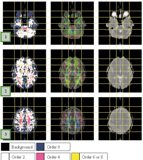
Figure 4 shows maps of the order chosen by our model selection procedure (left) for three axial slices of one of our data sets (results from the other data sets can be found in Ref. 23), together with mean diffusivity (right) and anisot-ropy-weighted color maps indicating the principal direc-tion of the DT at each point (middle). In the images in the middle column, the red, green, and blue intensities corre-spond to the size of thex,y, andzcomponents of the DT principal direction unit vector, weighted by the fractional anisotropy (2) as proposed by Pajevic and Pierpaoli (18).
A detailed anatomical analysis of the results is beyond the scope of this work, but we will highlight some inter-esting features. First, our procedure appears to separate regions of isotropic and anisotropic diffusion successfully. Regions of GM are mostly assigned order zero models, while regions of WM, both dense and peripheral, are mostly assigned order 2. A significant percentage of voxels are assigned higher order models. The spatial distribution of these voxels exhibits distinct clusters in the image, which have clear symmetry about the midline of the brain. The clustering and symmetry strongly suggest that the higher-order models correspond to genuine anatomical ef-fects.
Each slice shown in Fig. 4 contains an anatomic region that contains clusters of higher-order voxels consistently in each of our four data sets. In the top slice, the region corresponding to the pons contains a dense cluster of order 4 voxels (label 1). In this region, the right–left trans-pon-tine tracts cross the inferior-superior pyramidal tracts, causing partial volume effects between these two orthog-onal fibers. In the middle slice, dense clusters of order 4 voxels are found in the optic radiation on both sides of the brain (label 2). These occur precisely at the points where the anterior–posterior tracts of the optic radiation cross the predominantly right–left fibers of the corpus callosum. In the bottom slice, large clusters of order
4 voxels can be observed within the corona radiata (label 3). Again this is reasonable to expect, since the diverging fibers of the corona radiation are crossed by U-fibers in these areas.
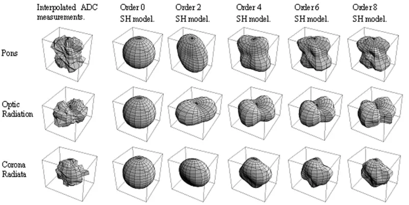
Figure 5 shows typical ADC profiles from each of these three regions, together with the order 0, 2, 4, 6, and 8 SH models. In each case, it is clear that there is significant difference between the order 4 and order 2 models, which indicates significant non-Gaussian behavior. The models with order greater than 4 do not appear to change the overall profile shape significantly further, and serve only to incorporate noise effects. The measurement from the pons is particularly striking and is typical of that predicted by the bi-Gaussian model for two orthogonally intersecting WM fibers (see Fig. 1). The measurement from the optic radiation is similar but oriented within the axial plane and somewhat less pronounced, possibly due to a less bal-anced mix between the two fibers, or a smaller angle of intersection. The profile from the corona radiata is more difficult to interpret, and may be the result of effects that are not modeled naturally by a bi-Gaussian model, such as fiber divergence or compartments with exchange.
Further Synthetic Experiments
Since the set of DTs tested in the synthetic experiments described in the Simulation Experiments section is not exhaustive, it is possible that the regions we observe in the human brain data simply exhibit Gaussian diffusion pro-cesses that are particularly prone to overfitting in our procedure. Thus, for completeness, we include an addi-tional set of experiments to test this assertion. In each region, we fit the DT (rather than the full SH series) at each voxel and model the distribution of DT eigenvalues,1⬎ 2⬎ 3, together with the value of0. We then use a Monte Carlo method to draw samples from this distribution and test the likelihood that the corresponding Gaussian ADC profiles are overfitted with SH models with order greater
than 2. 0 is included in this model, because the noise levels in ADC measurements depend on0as well as the magnitude of the ADC itself (19).
For each of the regions highlighted in the previous sec-tion (the pons, optic radiasec-tion, and corona radiata), a sub-region of the order 4 cluster was selected. A model of the distribution of DT shapes in each subregion was obtained by fitting a 4D multivariate Gaussian model to the distri-bution of vectors (1,2,3, and0). Our procedure was then applied to large numbers of samples drawn from each of these distributions, and the rate of classification above order 2 was found to be less than 5% in each case. These results verify that if the underlying diffusion process had been Gaussian, our procedure would have been effective and assigned most profiles in these regions order 2 models. Thus we conclude that we are observing genuine non-Gaussian effects in these regions.
DISCUSSION
We have described methods for modeling and detection of non-Gaussian ADC profiles and shown that such profiles can be observed with scanning parameters typical of stan-dard clinical DW-MRI data. The SH series up to order 8 was fit to samples of the ADC profile in each voxel, which provides a sequence of models of increasing com-plexity. A series of ANOVA tests was used to find the simplest of these models that adequately describes the data. This latter procedure classifies the profile at each voxel as isotropic, anisotropic Gaussian, or non-Gaussian, and allows maps of these different types of behavior to be produced, as shown in Fig. 4.
Our procedure was applied to human brain data col-lected with parameters typical of those used in clinical scans, and appeared to classify isotropic (GM) and aniso-tropic (WM) regions correctly as order 0 and order 2, respectively. On average, 5% of profiles in voxels within the brain were classified as order 4 or above (non-Gauss-ian). Several regions—in particular, the pons, optic radia-tion, and corona radiation—were found consistently to contain dense clusters of order 4 models. Validation of our method was performed by characterizing its performance using synthetic data with realistic noise properties, as well as applying it to DT models of data in regions of the brain that were consistently classified as non-Gaussian. Al-though results from only one data set are shown here, our method was applied to four data sets and other results can be found in Ref. 23. Acquisition of a larger ensemble of data sets is currently underway, which will enable para-metric mapping to be performed in order to allow compar-isons to be made between the occurrence of non-Gaussian diffusion in different population groups.
The behavior maps produced by our method provide new insights into the complexity of tissue structure in the brain. These maps have a number of practical applications. As mentioned in the Introduction, one aim is to use these maps as a stain for diagnosis of structure-reducing pathol-ogy. Furthermore, these maps can be used in postprocess-ing algorithms, such as tractography algorithms, which need to identify when diffusion is anisotropic and when the principal direction of the DT can be relied upon to describe the orientation of the underlying tissue. Finally,
these maps indicate when a more complex model (for example, a bi-Gaussian model) than the DT needs to be used to describeptadequately. Typically, such models are more difficult to fit to data than the DT and nonlinear fitting algorithms must be employed (see for example Ref. 21). Such procedures are computationally expensive, so it is advantageous to be able to identify only when they need to be performed.
It seems likely that most of the non-Gaussian behavior we observe is due to the intersection of WM fibers with different orientation. This kind of tissue structure gives rise to profiles similar to those that are derived from multi-Gaussian pt’s (22), although it is also likely that some exchange of particles between the tissue compartments corresponding to each fiber occurs in the timescale of the diffusion measurement, which will cause pt to deviate from the multi-Gaussian (22). Other types of non-Gaussian processes almost certainly occur in the brain, caused by restriction due to impermeable barriers (22). However, the deviation from Gaussian that is caused by these effects is less marked than those due to multicompartmentation, so such behavior may not be observed reliably—particularly at lowb-values such as those used here.
The advantages of the SHs as models for ADC profiles lie both in their generality and in the simplicity and robust-ness of the fitting procedure. Linearity of the fitting proce-dure is a significant advantage in terms of computational effort, but also ensures that the fitting procedure is well posed and is not prone to spurious erroneous results. There is littlephysicaljustification for the use of the SHs in this context, and there may be more appropriate sets of basis functions that better reflect the kind of ADC profiles that are likely to arise given the underlying physical pro-cesses. An advantage of this series, however, is its gener-ality: any profile can be represented, and we do not limit ourselves to particular models of the underlying processes. We note for clarity that whenptis non-Gaussian the shape of the ADC profile does not relate toptin a straightforward way, and thus the SH shape does not provide any direct information about the underlying tissue structure. Al-though it is possible to extract some information of this type from non-Gaussian profiles on the sphere (21), this issue is beyond the scope of this work.
There are many techniques for model selection in the literature. The use of ANOVA and theF-test for deletion of variables has proved more successful than most in our application, but there may be others that improve perfor-mance to some extent. The test we used is based on an assumption of Gaussian errors in the measurements. Al-though this is a reasonable first approximation for our data (23), the full analytic form of the errors in ADC measure-ments is not Gaussian. There are tests that incorporate noise models for the data, which may improve classifica-tion performance, particularly in extreme cases such as very anisotropic diffusion. We note that the same tech-nique could be used to produce a finer classification of diffusion profiles; for example, we could distinguish be-tween axisymmetric (two eigenvalues equal) and nonsym-metric (all eigenvalues unequal), anisotropic Gaussian dif-fusion.
our goals was to demonstrate that significant non-Gaussian behavior can be observed at b-values as low as 1000 s/mm2. Recently there has been a trend to move toward higherb-values, which can produce profiles richer in information; in particular, non-Gaussian behavior be-comes more pronounced (10). Our methods are equally applicable to data acquired with higherb-values, and we would expect to observe a higher proportion of non-Gaus-sian profiles in such data, which may highlight other re-gions of the brain in which non-Gaussian behavior occurs.
ACKNOWLEDGMENTS
Gareth Barker is funded by the Multiple Sclerosis Society of Great Britain and Northern Ireland. Thanks to Dr. Clau-dia Wheeler-Kingshott and Dr. Philip Boulby for pulse sequence development, and to Dr. Olga Ciccarelli for pro-viding data and aiding in the initial interpretation of the results.
REFERENCES
1. Basser PJ, Matiello J, Le Bihan D. MR diffusion tensor spectroscopy and imaging. Biophys J 1994;66:259 –267.
2. Basser PJ, Pierpaoli C. Microstructural and physiological features of tissues elucidated by quantitative diffusion tensor MRI. J Magn Reson B 1996;111:209 –219.
3. Pierpaoli C, Jezzard P, Basser PJ, Barnett A, Di Chiro G. Diffusion tensor MR imaging of the human brain. Radiology 1996;201:637– 648. 4. Callaghan PT. Principles of magnetic resonance microscopy. Oxford,
UK: Oxford Science Publications; 1991.
5. Karger J, Pfeifer H, Heink W. Principles and applications of self diffu-sion measurements by nuclear magnetic resonance. Adv Magn Reson 1988;12:1– 89.
6. Mitra PP, Halperin BI. Effects of finite gradient pulse widths in pulsed field gradient diffusion measurements. J Magn Reson 1995;113:94 –101. 7. Crank J. The mathematics of diffusion. Oxford, UK: Oxford University
Press; 1975.
8. Stejskal EO, Tanner JE. Spin diffusion measurements: spin echoes in the presence of time-dependent field gradient. J Chem Phys 1965;42: 288 –292.
9. Jones DK, Horsfield MA, Simmons A. Optimal strategies for measuring diffusion in anisotropic systems by magnetic resonance imaging. Magn Reson Med 1999;42:515–525.
10. Alexander AL, Hasan KM, Lazar M, Tsuruda JS, Parker DL. Analysis of partial volume effects in diffusion-tensor MRI. Magn Reson Med 2001; 45:770 –780.
11. Frank LR. Characterization of anisotropy in high angular resolution diffusion weighted MRI. In: Proceedings of the 9th Annual Meeting of ISMRM, Glasgow, Scotland, 2001. p 1531.
12. Tuch DS, Weisskoff RM, Belliveau JW, Wedeen VJ. High angular reso-lution diffusion imaging of the human brain. In: Proceedings of the 7th Annual Meeting of ISMRM, Philadelphia, 1999. p 321.
13. Wedeen VJ, Reese TG, Tuch DS, Weigel MR, Dou J-G, Weisskoff RM, Chesler D. Mapping fiber orientation spectra in cerebral white matter with Fourier transform diffusion MRI. In: Proceedings of the 8th An-nual Meeting of ISMRM, Denver, 2000. p 82.
14. Frank LR. Anisotropy in high angular resolution diffusion-weighted MRI. Magn Reson Med 2001;45:935–939.
15. Nikiforov AF, Uvarov VB. Special functions of mathematical physics. Basel: Birkhauser Verlag; 1988.
16. Brechbuhler CH, Gerig G, Kubler O. Parametrization of closed surfaces for 3D shape description. Comput Vis Image Underst 1995;61:154 –170. 17. Armitage P, Berry G. Statistical methods in medical research. Oxford,
UK: Blackwell Scientific Publications; 1971.
18. Pajevic S, Pierpaoli C. Color schemes to represent the orientation of anisotropic tissues from diffusion tensor data: application to white matter fiber tract mapping in the human brain. Magn Reson Med 1999;42:526 –540.
19. Armitage PA, Bastin ME. Utilizing the diffusion-to-noise ratio to opti-mize magnetic resonance diffusion tensor acquisition strategies for improving measurements of diffusion anisotropy. Magn Reson Med 2001;45:1056 –1065.
20. Alexander DC, Barker GJ, Arridge SR. Detection and modelling of non-Gaussianity in MR diffusion imaging. UCL, Department of Com-puter Science Research Note, RN/01/35, 2001. http://www.cs.ucl. ac.uk/staff/D.Alexander/Papers/RN35–2001.pdf
21. Alexander DC, Jansons KM. Spin echo attenuation to diffusion dis-placement density: a general inversion for measurements on a sphere. In: Proceedings of the ISMRM Workshop on Diffusion MRI: Biophysi-cal issues (what can we measure?), St. Malo, France, 2002.
22. Le Bihan D. Molecular diffusion, tissue microdynamics and micro-structure. NMR Biomed 1995;8:375–386.
![FIG. 1. Simulated examples of ADC profiles. Top row: profiles corresponding to Gaussian diffusion processes: (i) prolate DT oriented alongthe x-axis (eigenvalues [1700, 200, 200] �10–6 mm2/s), (ii) prolate DT oriented along the z-axis (eigenvalues [200, 200,](https://thumb-us.123doks.com/thumbv2/123dok_us/7899414.1311254/3.596.102.494.70.331/simulated-proles-proles-corresponding-gaussian-diffusion-eigenvalues-eigenvalues.webp)