Adaptive Central Force Optimization Algorithm Based on the Stability Analysis

(1)

Research Article

Adaptive Central Force Optimization Algorithm

Based on the Stability Analysis

Weiyi Qian,

1

Bo Wang,

1

and Zhiguang Feng

2

1_{College of Mathematics and Physics, Bohai University, Jinzhou 121000, China}

2_{College of Information Science and Technology, Bohai University, Jinzhou 121000, China}

Correspondence should be addressed to Weiyi Qian; [email protected]

Received 15 October 2014; Revised 20 February 2015; Accepted 26 February 2015

Academic Editor: Farhang Daneshmand

Copyright © 2015 Weiyi Qian et al. This is an open access article distributed under the Creative Commons Attribution License, which permits unrestricted use, distribution, and reproduction in any medium, provided the original work is properly cited.

In order to enhance the convergence capability of the central force optimization (CFO) algorithm, an adaptive central force optimization (ACFO) algorithm is presented by introducing an adaptive weight and defining an adaptive gravitational constant. The adaptive weight and gravitational constant are selected based on the stability theory of discrete time-varying dynamic systems. The convergence capability of ACFO algorithm is compared with the other improved CFO algorithm and evolutionary-based algorithm using 23 unimodal and multimodal benchmark functions. Experiments results show that ACFO substantially enhances the performance of CFO in terms of global optimality and solution accuracy.

1. Introduction

Consider the following global optimization problem:

max 𝑓 (𝑥)

subject to 𝑥 ∈ Ω = {𝑥 ∈ 𝑅𝑁𝑑| 𝑅min≤ 𝑥 ≤ 𝑅max} , (1)

where 𝑓(𝑥) : Ω ⊂ 𝑅𝑁𝑑 → 𝑅 _{is a real-valued}

bounded function and𝑅min,𝑅max, and𝑥are𝑁_𝑑-dimensional continuous variable vectors. Such problem arises in many applications, for example, in risk management, applied sci-ences, and engineering design. The function of interest may be nonlinear and nonsmooth which makes the classical optimization algorithms easily fail to solve these problems. Over the last decades, many nature-inspired heuristic opti-mization algorithms without requiring much information about the function became the most widely used optimization methods such as genetic algorithms (GA) [1], particle swarm optimization (PSO) [2], ant colony optimization (ACO) [3], cuckoo search (CS) algorithm [4], group search optimizer (GSO) [5], and glowworm swarm optimization (GSO1) [6]. These search methods all simulate biological phenomena. Different from these algorithms, some heuristic optimiza-tion algorithms based on physical principles have been developed, for example, simulating annealing (SA) algorithm

[7], electromagnetism-like mechanism (EM) algorithm [8], central force optimization (CFO) algorithm [9], gravitational search algorithm (GSA) [10], and charged system search (CSS) [11]. SA simulates solid material in the annealing process. EM is based on Coulomb’s force law associated with electrical charge process. GSA and CFO utilize New-tonian mechanics law. CSS is based on Coulomb’s force and Newtonian mechanics laws. Unlike other algorithms, CFO is a deterministic method. In other words, there is not any random nature in CFO, which attracts our attention on the CFO algorithm in this paper.

CFO, which was introduced by Formato in 2007 [9], is becoming a novel deterministic heuristic optimization algorithm based on gravitational kinematics. In order to improve the CFO algorithm, Formato and other researchers developed many versions of the CFO algorithm [12–23]. In [12,13], Formato proposed PR-CFO (Pseudo-Random CFO) algorithm. The improved implementations are made in three areas: initial probe distribution, repositioning factor, and decision space adaptation. Formato presented an algorithm known as PF-CFO (Parameter Free CFO) in [14,15]. PF-CFO algorithm improves and perfects the PR-CFO algorithm in the aspect of the selection of parameter. Mahmoud proposed an efficient global hybrid optimization algorithm combining the CFO algorithm and the Nelder-Mead (NM) method in Volume 2015, Article ID 914789, 10 pages

(2)

[16]. This hybrid method is called CFO-NM. An extended CFO (ECFO) algorithm was presented by Ding et al. by adding the historical information and defining an adaptive mass in [17] where the convergence of ECFO algorithm was proved based on the second order difference equation.

In aforementioned CFO algorithms, two updated equa-tions were used: one for a probe’s acceleration and the other for its position. In the probe’s position updated equation which is established based on the laws of motion, the velocity is defined as zero. But the velocity has influence on the exploring ability of the CFO algorithm. Therefore, in this paper, we introduce the velocity in the probe’s position updated equation, which leads us to build a velocity updated equation like the CSS algorithm. Since the weight which can balance the global and local search ability is an important parameter in many heuristic algorithms, we introduce weight in probe’s position updated equation. If the value of weight is too large, then the probes may move erratically, going beyond a good solution. On the other hand, if weight is too small, then the probe’s movement is limited and the optimal solution may not be reached. Therefore, an appropriate dynamically changing weight can improve the performance of the heuristic algorithm. However, in most of the heuristic algorithms, the changing weight was selected empirically according to the characteristics of the problems without theoretical analysis. The gravitational constant has the same effect on the weight in CFO algorithm. Hence, this paper will further investigate the weight and gravitational constant settings by employing the geometry-velocity stability theory of discrete time-varying dynamic systems. Based on the above discussion, an adaptive CFO (ACFO) algorithm is proposed in this paper.

To the best of our knowledge, there is no research on stability analysis of the CFO algorithm till now. In this paper, the stability of the ACFO algorithm is analyzed based on discrete time-varying dynamic systems theory. Based on the stability analysis of the proposed algorithm, we explore the weight and gravitational constant settings.

The rest of this paper is organized as follows.Section 2

will present the basics of the CFO algorithm and review the state of the art concerning the algorithm. InSection 3, we propose an adaptive central force optimization. Some numerical results are given to test the performance of the proposed algorithm in Section 4. Finally, we have some conclusions about the proposed algorithm.

2. Central Force Optimization

CFO solves problem(1)based on the movement of probes through the decision space (DS) along trajectories computa-tion by utilizing the gravitacomputa-tional analogy. The DS is defined byΩ = {(𝑥₁, 𝑥₂, . . . , 𝑥_𝑁𝑑) | 𝑅min_𝑖 ≤ 𝑥_𝑖≤ 𝑅max_𝑖 ,1≤ 𝑖 ≤ 𝑁_𝑑}. In CFO, a group of probes are represented as potential solutions, and each probe𝑝 is associated with position vector 𝑅𝑝(𝑡) and acceleration vector𝐴𝑝(𝑡)at time step𝑡. The position of each probe is initialized by a variable initial probe distribution formed by deploying𝑁_𝑝/𝑁_𝑑probes uniformly on each of the probe lines parallel to the coordinate axes and intersecting at a point alongΩ’s principal diagonal, where𝑁_𝑝is the total

number of initial probes. The initial acceleration vectors are usually set to zero. During search process, the acceleration and position of probe𝑝are updated as

𝐴𝑝_𝑖(𝑡) = 𝐺

𝑁𝑝

∑

𝑘=1

𝑘 ̸=𝑝

𝑈 (𝑀𝑘(𝑡) − 𝑀𝑝(𝑡)) (𝑀𝑘(𝑡) − 𝑀𝑝(𝑡))𝛼

⋅ (𝑅

𝑘

𝑖 (𝑡) − 𝑅𝑝𝑖 (𝑡))

󵄩󵄩󵄩󵄩𝑅𝑘_{(𝑡) − 𝑅}𝑝_{(𝑡)󵄩󵄩󵄩󵄩}𝛽,

(2)

𝑅𝑝_𝑖 (𝑡 +1) = 𝑅𝑝_𝑖 (𝑡) +1 2𝐴

𝑝

𝑖 (𝑡) Δ𝑡2, (3)

where𝐺is the gravitational constant;𝑀𝑗(𝑡) = 𝑓(𝑅𝑗(𝑡))is the fitness value at probe𝑗’s(𝑗 = 1,2, . . . , 𝑁_𝑝)position at time step𝑡;𝛼and𝛽are the parameters;𝑖 (𝑖 =1,2, . . . , 𝑁_𝑑)is the coordinate number;𝑈(⋅)is the unit step function;

𝑈 (𝑧) ={_{ {

1, 𝑧 ≥0

0, else; (4)

Δ𝑡is the unit time step increment; define‖𝑅𝑘(𝑡) − 𝑅𝑝(𝑡)‖ =

√∑𝑁𝑑

𝑖=1[𝑅𝑖𝑘(𝑡) − 𝑅𝑝𝑖(𝑡)]2. The probe generated by (3)may be

beyond the DS. If the coordinate 𝑅𝑝_𝑖(𝑡 + 1) of the probe

𝑅𝑝_{(𝑡 +}₁₎_{is less than}_𝑅min

𝑖 , then it is assigned to be

𝑅𝑝_𝑖 (𝑡 +1) = 𝑅_𝑖min+ 𝐹_rep[𝑅𝑝_𝑖 (𝑡 −1) − 𝑅min_𝑖 ] . (5)

If𝑅𝑝_𝑖(𝑡 +1)is greater than𝑅max_𝑖 , then

𝑅𝑝_𝑖 (𝑡 +1) = 𝑅max_𝑖 − 𝐹_rep[𝑅min_𝑖 − 𝑅𝑝_𝑖 (𝑡 −1)] , (6)

where 𝑅_𝑖min and 𝑅max_𝑖 are the minimum and maximum values for𝑖th component of the decision variable.𝐹_repis the reposition factor which starts at an arbitrary initial value

𝐹initial

rep <1 and is incremented by an arbitrary amountΔ𝐹rep

at each iteration. If𝐹_rep ≥ 1, then it is reset to the starting value. In order to improve convergence speed, the DS size is adaptively reduced around the best probe𝑅_best. The DS’s boundary coordinates are reduced as follows:

𝑅min_𝑖 = 𝑅min_𝑖 +1

2[𝑅best− 𝑅

min

𝑖 ] ,

𝑅max_𝑖 = 𝑅max_𝑖 −1

2[𝑅

max

𝑖 − 𝑅best] .

(7)

The termination criterion is that iterations reach their max-imum limit𝑁_𝑡. We also terminate the CFO algorithm early if the difference between the average best fitness over𝑞steps (including the current step) and the current best fitness is less than 10−6.

In order to improve the CFO algorithm, Formato pro-posed modifications to CFO algorithm, namely, PR-CFO [12, 13]. The steps of PR-CFO algorithm [13] are shown as follows;

(3)

For𝛾 = 𝛾_startto𝛾_stopbyΔ𝛾

(a.1) compute initial probe distribution with distri-bution factor𝛾;

(a.2) compute initial fitness matrix; select the best probe fitness;

(a.3) assign initial probe acceleration; (a.4) set initial𝐹_rep= 𝐹_repinit.

For𝑡 =0 to𝑁_𝑡(or earlier termination criterion)

(b) update probe positions using(3); (c) retrieve errant probe using(5)and(6);

(d) calculate fitness values; select the best probe fitness;

(e) compute accelerations using(2); (f) increment𝐹_repbyΔ𝐹_best;

if𝐹_rep>1 then𝐹_rep= 𝐹_repmin; End If

(g) if𝑡MOD 10 = 0, then

shrinkΩaround best probe using(7); End If

Next𝑡

(h) reset Ω’s boundaries to their starting values before shrinking.

Next𝛾

Next𝑁_𝑝/𝑁_𝑑.

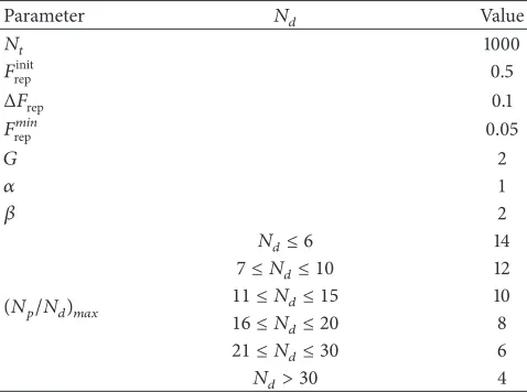
PR-CFO is further modified in order to create an algorithm known as PF-CFO (Parameter Free CFO) [14, 15]. This version is almost identical to PR-CFO and compensates for the number of parameters that must be chosen by fixing a wide array of internal parameters at specific values [19]. The values of parameters borrowed from [19] that are used in PF-CFO algorithm can be seen inTable 1.

3. Adaptive Central Force

Optimization Algorithm

Qian and Zhang [23] proposed an adaptive central force optimization algorithm. In [23], the time Δ𝑡 in (3) was updated based on the fitness value compared with the average fitness value. In this paper, we introduce adaptive weight in position update equation, adaptive gravitational constant in acceleration update equation and the velocity update formula. The weight and gravitational constant are

Table 1: The values of parameters that are used in PF-CFO algorithm.

Parameter 𝑁_𝑑 Value

𝑁_𝑡 1000

𝐹init

rep 0.5

Δ𝐹rep 0.1

𝐹𝑚𝑖𝑛

rep 0.05

𝐺 2

𝛼 1

𝛽 2

(𝑁_𝑝/𝑁_𝑑)_𝑚𝑎𝑥

𝑁_𝑑≤6 14

7≤ 𝑁_𝑑≤10 12

11≤ 𝑁_𝑑≤15 10

16≤ 𝑁_𝑑≤20 8

21≤ 𝑁_𝑑≤30 6

𝑁𝑑>30 4

updated based on this stability analysis of a discrete time-varying dynamic system. In ACFO algorithm, the position, acceleration, and velocity of probe𝑝are updated as follows:

𝑅𝑝_𝑖 (𝑡 +1) = 𝑅𝑝_𝑖 (𝑡) + 𝜔𝑝(𝑡) 𝑉_𝑖𝑝(𝑡) Δ𝑡 +1 2𝐴

𝑝

𝑖(𝑡) Δ𝑡2, (8)

𝐴𝑝_𝑖(𝑡 +1) = 𝐺𝑝(𝑡 +1)

𝑁𝑝

∑

𝑘=1

𝑘 ̸=𝑝

𝑈 (𝑀𝑘(𝑡 +1) − 𝑀𝑝(𝑡 +1))

⋅ (𝑀𝑘(𝑡 +1) − 𝑀𝑝(𝑡 +1))𝛼

⋅(𝑅

𝑘

𝑖 (𝑡 +1) − 𝑅𝑝𝑖 (𝑡 +1))

(𝐷_𝑝𝑘)𝛽 ,

(9)

𝑉_𝑖𝑝(𝑡 +1) = 𝑅

𝑝

𝑖 (𝑡 +1) − 𝑅𝑖𝑝(𝑡)

Δ𝑡 , (10)

where𝜔𝑝(𝑡)is the weight;𝐺𝑝(𝑡) is a gravitational constant at probe𝑝’s position at iteration𝑡;Δ𝑡 = 1;𝛼and𝛽are the parameters;𝑖 (𝑖 =1,2, . . . , 𝑁_𝑑)is the coordinate number; and

𝐷_𝑝𝑘is defined as follows:

𝐷_𝑝𝑘={_{ {

𝑑_𝑝𝑘, if 𝑑_𝑝𝑘≥ 𝑎

𝑎, if 𝑑_𝑝𝑘< 𝑎, (11)

where𝑑_𝑝𝑘 is the Euclidian distance between two probes,𝑝 and𝑘, and𝑎is a radius constant.

Let

𝜑_𝑘(𝑡) = 𝑈 (𝑀

𝑘_{(𝑡) − 𝑀}𝑝_{(𝑡)) (𝑀}𝑘_{(𝑡) − 𝑀}𝑝_(𝑡))𝛼

(𝐷𝑝𝑘)𝛽

,

𝜑 (𝑡) =

𝑁𝑝

∑

𝑘=1

𝑘 ̸=𝑝

𝜑_𝑘(𝑡) .

(4)

It is clear that 𝜑_𝑘(𝑡) and 𝜑(𝑡) are nonnegative. By (8), (9), and(10), the position and velocity updated equations can be written as follows:

𝑅𝑝_𝑖 (𝑡 +1) = (1−1 2𝐺 𝑝_{(𝑡) 𝜑 (𝑡)) 𝑅}𝑝 𝑖 (𝑡) + 𝜔𝑝(𝑡) 𝑉𝑖𝑝(𝑡) +1 2𝐺 𝑝_(𝑡)_∑𝑁𝑝 𝑘=1 𝑘 ̸=𝑝 𝜑_𝑘(𝑡) 𝑅𝑘_𝑖(𝑡) ,

𝑉_𝑖𝑝(𝑡 +1) = −1 2𝐺 𝑝_{(𝑡) 𝜑 (𝑡) 𝑅}𝑝 𝑖 (𝑡) + 𝜔𝑝(𝑡) 𝑉𝑖𝑝(𝑡) +1 2𝐺 𝑝_(𝑡)_∑𝑁𝑝 𝑘=1 𝑘 ̸=𝑝 𝜑_𝑘(𝑡) 𝑅𝑘_𝑖(𝑡) . (13)

Equations(13)are written in matrix form as follows:

(𝑅

𝑝

𝑖 (𝑡 +1)

𝑉_𝑖𝑝(𝑡 +1)) = ( 1−1

2𝐺 𝑝_{(𝑡) 𝜑 (𝑡) 𝜔}𝑝_(𝑡) −1 2𝐺 𝑝_{(𝑡) 𝜑 (𝑡) 𝜔}𝑝_(𝑡)) ( 𝑅𝑝_𝑖 (𝑡) 𝑉_𝑖𝑝(𝑡)) +1 2𝐺 𝑝_{(𝑡) (}₍ ( 𝑁𝑝 ∑ 𝑘=1 𝑘 ̸=𝑝 𝜑_𝑘(𝑡) 𝑅𝑘 𝑖 (𝑡) 𝑁𝑝 ∑ 𝑘=1 𝑘 ̸=𝑝 𝜑_𝑘(𝑡) 𝑅𝑘 𝑖 (𝑡) ) ) ) . (14) Let

𝑥 (𝑡 +1) = (𝑅

𝑝

𝑖 (𝑡 +1)

𝑉_𝑖𝑝(𝑡 +1)) ,

𝑔 (𝑡, 𝑥 (𝑡)) = (1−

1 2𝐺 𝑝_{(𝑡) 𝜑 (𝑡) 𝜔}𝑝_(𝑡) −1 2𝐺 𝑝_{(𝑡) 𝜑 (𝑡) 𝜔}𝑝_(𝑡)) ( 𝑅𝑝_𝑖 (𝑡) 𝑉_𝑖𝑝(𝑡)) +1 2𝐺 𝑝_{(𝑡) (}₍ ( 𝑁𝑝 ∑ 𝑘=1 𝑘 ̸=𝑝 𝜑_𝑘(𝑡) 𝑅𝑘_𝑖(𝑡) 𝑁𝑝 ∑ 𝑘=1 𝑘 ̸=𝑝 𝜑_𝑘(𝑡) 𝑅𝑘_𝑖(𝑡) ) ) ) . (15)

Equation(14) can be expressed as a discrete time-varying dynamic system as follows:

𝑥 (𝑡 +1) = 𝑔 (𝑡, 𝑥 (𝑡)) , 𝑡 =1,2, . . . . (16)

Lemma 1 (see [24]). Let𝑥(𝑡+1) = 𝑔(𝑡, 𝑥(𝑡))be a discrete

time-varying dynamic system; if𝑔(𝑡, 𝑥(𝑡))satisfies the condition

󵄩󵄩󵄩󵄩𝑔(𝑡,𝑥(𝑡))󵄩󵄩󵄩󵄩𝜐≤V(𝑡) ‖𝑥 (𝑡)‖𝜐+ 𝑐, (17)

under a certain vector norm‖ ⋅ ‖_𝜐, then the system is

geometry-velocity stable in the bounded set𝐿 = {𝑥 | ‖𝑥‖_𝜐 < 𝑐/(1− 𝜗)},

where𝑐is constant and0≤V(𝑡) ≤ 𝜗 <1.

Cui and Zen presented a selection of the parameters in PSO algorithm based on Lemma 1 in [24]. Now we analyze the stability of ACFO algorithm and give a selection of weight and gravitational constant based onLemma 1.

If‖⋅‖_𝜐inLemma 1is considered as an infinite norm, then we have 󵄩󵄩󵄩󵄩𝑔(𝑡,𝑥(𝑡))󵄩󵄩󵄩󵄩∞≤ 󵄩󵄩󵄩󵄩 󵄩󵄩󵄩󵄩 󵄩󵄩󵄩󵄩 󵄩󵄩

(1−

1 2𝐺 𝑝_{(𝑡) 𝜑 (𝑡) 𝜔}𝑝_(𝑡) −1 2𝐺 𝑝_{(𝑡) 𝜑 (𝑡) 𝜔}𝑝_(𝑡)) 󵄩󵄩󵄩󵄩 󵄩󵄩󵄩󵄩 󵄩󵄩󵄩󵄩 󵄩󵄩∞ ‖𝑥 (𝑡)‖∞ +1 2󵄨󵄨󵄨󵄨𝐺 𝑝 (𝑡)󵄨󵄨󵄨󵄨 󵄩󵄩󵄩󵄩 󵄩󵄩󵄩󵄩 󵄩󵄩󵄩󵄩 󵄩󵄩󵄩󵄩 󵄩󵄩󵄩󵄩 󵄩󵄩󵄩󵄩 󵄩󵄩󵄩 ( ( ( 𝑁𝑝 ∑ 𝑘=1 𝑘 ̸=𝑝 𝜑_𝑘(𝑡) 𝑅𝑘 𝑖(𝑡) 𝑁𝑝 ∑ 𝑘=1 𝑘 ̸=𝑝 𝜑_𝑘(𝑡) 𝑅𝑘 𝑖(𝑡) ) ) ) 󵄩󵄩󵄩󵄩 󵄩󵄩󵄩󵄩 󵄩󵄩󵄩󵄩 󵄩󵄩󵄩󵄩 󵄩󵄩󵄩󵄩 󵄩󵄩󵄩󵄩 󵄩󵄩󵄩∞ . (18)

Since𝐺𝑝(𝑡)is a nonnegative finite number for any𝑡and

𝑓(⋅)is a bounded function, we assume that𝐺𝑝(𝑡) ≤ 𝐺and

‖𝑓(⋅)‖ ≤ 𝑀 =max_𝑥∈Ω|𝑓(𝑥)|. Thus, we can obtain

0≤ 𝑈 (𝑀𝑘(𝑡) − 𝑀𝑝(𝑡)) (𝑀𝑘(𝑡) − 𝑀𝑝(𝑡))𝛼≤ 𝑀𝛼. (19)

By(11), one has𝐷_𝑝𝑘≥ 𝑎. Therefore, we have𝜑_𝑘(𝑡) ≤ 𝑀𝛼/𝑎𝛽. Thus, 1 2󵄨󵄨󵄨󵄨𝐺 𝑝 (𝑡)󵄨󵄨󵄨󵄨 󵄩󵄩󵄩󵄩 󵄩󵄩󵄩󵄩 󵄩󵄩󵄩󵄩 󵄩󵄩󵄩󵄩 󵄩󵄩󵄩󵄩 󵄩󵄩󵄩󵄩 󵄩󵄩󵄩 ( ( ( 𝑁𝑝 ∑ 𝑘=1 𝑘 ̸=𝑝 𝜑_𝑘(𝑡) 𝑅𝑘_𝑖 (𝑡) 𝑁𝑝 ∑ 𝑘=1 𝑘 ̸=𝑝 𝜑_𝑘(𝑡) 𝑅𝑘_𝑖 (𝑡) ) ) ) 󵄩󵄩󵄩󵄩 󵄩󵄩󵄩󵄩 󵄩󵄩󵄩󵄩 󵄩󵄩󵄩󵄩 󵄩󵄩󵄩󵄩 󵄩󵄩󵄩󵄩 󵄩󵄩󵄩∞ ≤ 1 2𝐺 󵄨󵄨󵄨󵄨 󵄨󵄨󵄨󵄨 󵄨󵄨󵄨󵄨 󵄨󵄨󵄨 𝑁𝑝 ∑ 𝑘=1 𝑘 ̸=𝑝 𝜑_𝑘(𝑡) 𝑅𝑘_𝑖 (𝑡)󵄨󵄨󵄨󵄨󵄨󵄨󵄨󵄨_{󵄨󵄨󵄨󵄨} 󵄨󵄨󵄨 ≤ 1 2𝐺 𝑁𝑝 ∑ 𝑘=1 𝑘 ̸=𝑝 𝜑𝑘(𝑡)󵄨󵄨󵄨󵄨_󵄨𝑅𝑘𝑖(𝑡)󵄨󵄨󵄨󵄨_󵄨

≤ (𝑁𝑝−1) 𝑀

𝛼

2𝑎𝛽

⋅ max

1≤𝑖≤𝑁𝑑{max{𝑅

max

𝑖 ,

−𝑅min_𝑖 }}.

(20) In addition, 󵄩󵄩󵄩󵄩 󵄩󵄩󵄩󵄩 󵄩󵄩󵄩󵄩 󵄩󵄩

(1−

1 2𝐺 𝑝_{(𝑡) 𝜑 (𝑡) 𝜔}𝑝_(𝑡) −1 2𝐺 𝑝_{(𝑡) 𝜑 (𝑡) 𝜔}𝑝_(𝑡)) 󵄩󵄩󵄩󵄩 󵄩󵄩󵄩󵄩 󵄩󵄩󵄩󵄩 󵄩󵄩∞

≤max{󵄨󵄨󵄨󵄨_󵄨󵄨󵄨1−1 2𝐺

𝑝(𝑡) 𝜑 (𝑡)󵄨󵄨󵄨󵄨

󵄨󵄨󵄨 + 𝜔𝑝(𝑡) , 󵄨󵄨󵄨󵄨

󵄨󵄨󵄨−12𝐺

𝑝(𝑡) 𝜑 (𝑡)󵄨󵄨󵄨󵄨

󵄨󵄨󵄨 + 𝜔𝑝(𝑡)} .

(5)

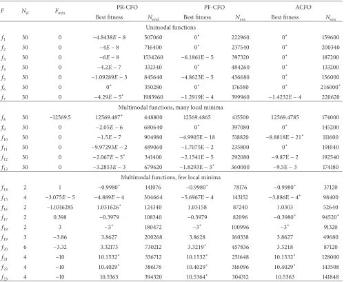
Table 2: Comparison of ACFO with RP-CFO and RF-CFO.

𝐹 𝑁𝑑 𝐹𝑚𝑖𝑛 PR-CFO PF-CFO ACFO

Best fitness 𝑁eval Best fitness 𝑁eva Best fitness 𝑁eva

Unimodal functions

𝑓1 30 0 −4.8438𝐸 − 8 507060 0∗ 222960 0∗ 159600

𝑓₂ 30 0 −4𝐸 − 8 716400 0∗ 237540 0∗ 200340

𝑓3 30 0 −6𝐸 − 8 1534260 −6.1861E−5 397320 0∗ 187200

𝑓4 30 0 −4.2𝐸 − 7 332340 0∗ 484260 0∗ 133200

𝑓₅ 30 0 −1.09289𝐸 − 3 845640 −4.8623E−5 436680 0∗ 156000

𝑓6 30 0 0∗ 350280 0∗ 176580 0∗ 216000∗

𝑓7 30 0 −4.29𝐸 − 5∗ 1983960 −1.2919E−4 399960 −1.4232E−4 220620

Multimodal functions, many local minima

𝑓8 30 −12569.5 12569.487∗ 448800 12569.4865 415500 12569.4785 174000

𝑓₉ 30 0 −2.05𝐸 − 6 680640 0∗ 397080 0∗ 145200

𝑓10 30 0 −1.5𝐸 − 7 904980 −4.9905E−18 518820 −8.8818E−21∗ 111600

𝑓11 30 0 −9.97293𝐸 − 2 489060 −1.7075E−2 235800 0∗ 191040

𝑓₁₂ 30 0 −2.067𝐸 − 5∗ 341400 −2.1541E−5 292080 −9.87E−2 192540

𝑓13 30 0 −3.2853𝐸 − 3 679620 −1.8293E−3∗ 360000 −9.5E−3 174180

Multimodal functions, few local minima

𝑓14 2 1 −0.9980∗ 141076 −0.9980∗ 78176 −0.9980∗ 37120

𝑓15 4 −3.075𝐸 − 5 −4.889𝐸 − 4 304664 −5.6967E−4 143152 −3.886E−4∗ 98400

𝑓₁₆ 2 −1.0316285 1.031626∗ 124340 1.03158 87240 1.0303 52640

𝑓17 2 0.398 −0.3979 108340 −0.3979 82096 −0.3980∗ 94520∗

𝑓18 2 3 −3∗ 180472 −3∗ 100996 −3∗ 91320

𝑓₁₉ 3 −3.86 3.8627 200268 3.8628 160338 3.8627 49680

𝑓20 6 −3.32 3.32173 730212 3.3219∗ 457836 3.3218 87120

𝑓21 4 −10 10.1532∗ 336712 10.1532∗ 251648 10.1532∗ 128000

𝑓₂₂ 4 −10 10.4029∗ 386176 10.4029∗ 316096 10.4029∗ 143508

𝑓23 4 −10 10.5363 394320 10.5364∗ 304312 10.5363 141848

Set𝑐 = ((𝑁_𝑝−1)𝑀𝛼/2𝑎𝛽)max₁_{≤𝑖≤𝑁}_𝑑{max{𝑅max_𝑖 , −𝑅min_𝑖 }}. If

max{󵄨󵄨󵄨󵄨_󵄨󵄨󵄨1−1 2𝐺

𝑝(𝑡) 𝜑 (𝑡)󵄨󵄨󵄨󵄨

󵄨󵄨󵄨 + 𝜔𝑝(𝑡) ,󵄨󵄨󵄨󵄨󵄨󵄨󵄨−12𝐺

𝑝(𝑡) 𝜑 (𝑡)󵄨󵄨󵄨󵄨

󵄨󵄨󵄨 + 𝜔𝑝(𝑡)} ≤ 𝜃 <1,

(22)

then byLemma 1, system(16)is geometry-velocity stable in the bounded set𝐿 = {𝑥 | ‖𝑥‖_∞≤ 𝑐/(1− 𝜃)}.

By(22), one has 0< (1/2)𝐺𝑝(𝑡)𝜑(𝑡) <1. If 0< (1/2)𝐺𝑝(𝑡)

𝜑(𝑡) <0.5, that is, 0< 𝐺𝑝(𝑡) <1/𝜑(𝑡), then(1/2)𝐺𝑝(𝑡)𝜑(𝑡) +

𝜔𝑝_{(𝑡) <} ₁_{− (}₁_/₂_)𝐺𝑝_{(𝑡)𝜑(𝑡) + 𝜔}𝑝_{(𝑡) ≤ 𝜃}_{; that is, 0}_{< 𝜔}𝑝_{(𝑡) ≤}

(1/2)𝐺𝑝(𝑡)𝜑(𝑡) + 𝜃 −1. If 0.5 ≤ (1/2)𝐺𝑝(𝑡)𝜑(𝑡) < 1, that is, 1/𝜑(𝑡) ≤ 𝐺𝑝(𝑡) < 2/𝜑(𝑡), then 1− (1/2)𝐺𝑝(𝑡)𝜑(𝑡) + 𝜔𝑝(𝑡) ≤

(1/2)𝐺𝑝(𝑡)𝜑(𝑡) + 𝜔𝑝(𝑡) ≤ 𝜃; that is, 0 < 𝜔𝑝(𝑡) ≤ 𝜃 −

(1/2)𝐺𝑝(𝑡)𝜑(𝑡).

From the above discussion, in order to guarantee the geometry-velocity stability of system(16), parameters𝜔𝑝(𝑡) and𝐺𝑝(𝑡)are selected as follows:

𝐺𝑝(𝑡) = 2

𝜑 (𝑡)rand(0,1) ,

𝜔𝑝_{(𝑡) =}

{ { { { { { { { { { { { { { { { { { { { {

(1

2𝐺

𝑝_{(𝑡) 𝜑 (𝑡) + 𝜃 −}₁₎_rand₍₀_,₁_{) ,}

if 0< 𝐺𝑝(𝑡) < 1

𝜑 (𝑡), (𝜃 −1

2𝐺

𝑝_{(𝑡) 𝜑 (𝑡))}_rand₍₀_,₁_{) ,}

if 1

𝜑 (𝑡)≤ 𝐺𝑝(𝑡) <

2

𝜑 (𝑡),

(23)

(6)

should not contain any random nature. Therefore, we take parameters𝜔𝑝(𝑡)and𝐺𝑝(𝑡)as follows:

𝐺𝑝(𝑡) =min{2, 𝜇 2

𝜑 (𝑡)} , (24)

𝜔𝑝(𝑡) = { { { { { { { { { { { { { { { { { { { { {

𝜂 (1

2𝐺

𝑝_{(𝑡) 𝜑 (𝑡) −}₀_.₁_{) ,}

if 0< 𝐺𝑝(𝑡) < 1

𝜑 (𝑡), 𝜂 (0.9−1

2𝐺

𝑝_{(𝑡) 𝜑 (𝑡)) ,}

if 1

𝜑 (𝑡)≤ 𝐺𝑝(𝑡) <

2

𝜑 (𝑡),

(25)

where𝜇and𝜂are two constants between 0 and 1.

The specific iterative steps of ACFO algorithm are listed as follows.

For𝑁_𝑝/𝑁_𝑑=2 to(𝑁_𝑝/𝑁_𝑑)_maxstep size is 2. For𝛾 = 𝛾_startto𝛾_stopbyΔ𝛾

(a.1) compute initial probe distribution with distri-bution factor𝛾;

(a.2) compute initial fitness matrix; select the best probe fitness;

(a.3) assign initial probe’s accelerations and velocities; (a.4) set initial𝐹_rep= 𝐹_repinitand𝐺init.

For𝑡 =0 to𝑁_𝑡(or earlier termination criterion)

(b) compute weights using(25); (c) update probe positions using(8); (d) retrieve errant probe using(5)and(6);

(e) calculate fitness values; select the best probe fitness;

(f) update gravitational constant using(24); (g) compute accelerations using(9)and velocities

using(10);

(h) increment𝐹_repbyΔ𝐹_best; if𝐹_rep>1 then𝐹_rep= 𝐹_repmin; End If

(i) if𝑡MOD 10 = 0, then

shrinkΩaround best probe using(7); End If

Next𝑡

(l) reset Ω’s boundaries to their starting values before shrinking.

Next𝛾 Next𝑁_𝑝/𝑁_𝑑.

In ACFO algorithm, the initial acceleration and velocities vectors are set to zero and ⃗𝑒 = ∑𝑁𝑑_𝑘=₁0.01 _𝑘⃗𝑒, where _𝑘⃗𝑒 is the unit vector along the𝑘-axis.

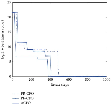
0 200 400 600 800 1000

0 2 4 6 8 10 12 14

Iterate steps

PR-CFO PF-CFO ACFO

log(

1+

be

st

fit

ness s

o fa

r)

Figure 1: Convergence curves of three algorithms on𝑓₁.

0 200 400 600 800 1000

0 10 20 30 40 50 60 70

Iterate steps

log(

1+

be

st

fit

ness s

o fa

r)

PR-CFO PF-CFO ACFO

Figure 2: Convergence curves of three algorithms on𝑓₂.

4. Numerical Experiments

In this section, the performance of ACFO algorithm is compared with the existing algorithms, GSO, GA, PSO, PR-CFO, PF-PR-CFO, CFO-NM, and EPSO, using a suite of the former twenty-three benchmark functions provided in [25]. In ACFO algorithm, internal parameters 𝛾_start = 0 and

(7)

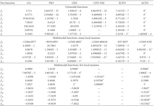
Table 3: Comparison of ACFO with GA, PSO, GSO, CFO-NM, and ECFO.

Test function GA PSO GSO CFO-NM ECFO ACFO

Unimodal functions

𝑓1 3.711 3.6927𝐸 − 37 1.9481𝐸 − 8 8.86597𝐸 − 25 7.5137𝐸 − 7 0∗

𝑓2 0.5771 2.9168𝐸 − 24 3.7039𝐸 − 5 9.46909𝐸 − 5 4.8954𝐸 − 7 0∗

𝑓₃ 9749.9145 1.1979𝐸 − 3 5.7829 5.89019𝐸 − 9 9.7713𝐸 − 7 0∗

𝑓₄ 7.9610 0.4123 10.7𝐸 − 2 6.40640𝐸 − 3 9.7203𝐸 − 7 0∗

𝑓5 338.5616 37.3582 49.8359 1.12593𝐸 − 7 4.3433𝐸 − 5 0∗

𝑓₆ 3.69701 0.1460 1.600𝐸 − 2 — 2.2016𝐸 − 7 0∗

𝑓₇ 0.1045 9.9024𝐸 − 3 7.3773𝐸 − 2 — 2.525𝐸 − 5∗ 1.4850𝐸 − 4

Multimodal functions, many local maxima

𝑓₈ −12566.0977 −9659.6993 −12569.4882∗ _{−12569.486618} _−837.9657 _{−12569.4785}

𝑓9 6.509𝐸 − 1 20.7863 1.0179 6.89347𝐸 − 23 7.5095𝐸 − 5 0∗

𝑓₁₀ 0.8678 1.3404𝐸 − 3 2.6548𝐸 − 5 1.49081𝐸 − 11 6.8426𝐸 − 5 8.8818𝐸 − 21∗

𝑓₁₁ 1.0038 0.2323 3.0792𝐸 − 2 4.99600𝐸 − 15 4.6279𝐸 − 5 0∗

𝑓12 4.3572𝐸 − 2 3.9503𝐸 − 2 2.7648𝐸 − 11 1.93296𝐸 − 21∗ 1.6471𝐸 − 5 9.87𝐸 − 2

𝑓₁₃ 0.1681 5.0519𝐸 − 2 4.6948𝐸 − 5∗ _— _{6.1817𝐸 − 5} _{9.5𝐸 − 3}

Multimodal functions, few local maxima

𝑓₁₄ 0.9989 1.0239 0.9980∗ _— _— _0.9980∗

𝑓₁₅ 7.0878𝐸 − 3 3.8074𝐸 − 4 3.7713𝐸 − 4∗ _— _— _{3.886𝐸 − 4}

𝑓16 −1.0298 −1.0160 −1.031628 −1.03163∗ — −1.0303

𝑓₁₇ 0.4040 0.4040 0.3979 0.39700∗ _— _0.3980

𝑓₁₈ 7.5027 3.0050 3∗ _3.00000∗ ₃∗

𝑓19 −3.8624 −3.8582 −3.8628 — — −3.8627

𝑓₂₀ −3.2627 −3.1846 −3.2697 — — −3.3218∗

𝑓₂₁ −5.1653 −7.5439 −6.09 — — −10.1532∗

𝑓22 −5.4432 −8.3553 −6.5546 — — −10.4029∗

𝑓₂₃ −4.9108 −8.9439 −7.4022 — — −10.5362∗

system. The stopping condition is that iterations reach their maximum limit𝑁_𝑡. We also early stop the ACFO algorithm if the difference between the average best fitness over 30 steps (including the current step) and the current best fitness is less than 10−6.

In Table 2, 𝐹, 𝑁_𝑑, 𝑓_min, and 𝑁_eval stand for the test function, the dimension of decision space, the optimum minimum value for each function, and the total number of function evaluations, respectively. The statistical data in

Table 2for RP-CFO and RF-CFO are reproduced from [13] and [15], respectively. The best fitness is the optimum maxi-mum (note the negative of each of the benchmark functions). The set of twenty-three benchmark functions are divided into unimodal functions (𝑓₁to𝑓₇), multimodal functions (𝑓₈to

𝑓₁₃), and low-dimensional multimodal functions (𝑓₁₄to𝑓₂₃).

Table 3summarizes the obtained optimum minimum results which are compared with other optimization algorithms, such as GA, PSO, GSO, CFO-NM, and ECFO. The statistical data for CFO-NM and ECFO is from [16,17] while the other statistical data is from [5]. In Tables 2 and 3, the star ∗ denotes that the numerical result is the best one among all the comparative algorithms. InTable 3, the symbol “—” means that the problem is not calculated in the original references.

From Table 2, it is clearly seen that the ACFO algo-rithm yields significantly better performance than PR-CFO

algorithm on benchmark functions 𝑓₁–𝑓₅. But the ACFO algorithm has a worse result on 𝑓₇ and same result on

𝑓₆compared to PR-CFO algorithm. From the comparisons between ACFO algorithm and PF-CFO algorithm, we can find that ACFO algorithm performs better than PF-CFO algorithm on𝑓₃and𝑓₅and obtains the same results yielded by PF-CFO algorithm on 𝑓₁, 𝑓₂, 𝑓₄, 𝑓₆, and 𝑓₇. But it should be noted that both the ACFO and PF-CFO algorithm can obtain optimum minimum value of 𝑓₁, 𝑓₂, 𝑓₄, and

𝑓6.

The set of benchmark functions𝑓₈–𝑓₁₃ are multimodal functions with many local minima. From Table 2, we can see that the ACFO algorithm outperforms PR-CFO and PF-CFO algorithm except functions 𝑓₈, 𝑓₁₂, and𝑓₁₃, but PR-CFO and PF-PR-CFO algorithm are superior to APR-CFO algorithm on benchmark function 𝑓₈ by a very small percentage of

6.683𝐸 − 07and6.285𝐸 − 07, respectively.

The other set of benchmark functions 𝑓₁₄–𝑓₂₃ are low dimensions multimodal functions. From the comparison shown inTable 2, it can be obviously seen that the best fitness generated by ACFO, PR-CFO, and PF-CFO algorithm are almost the same on𝑓₁₄–𝑓₂₃.

(8)

0 200 400 600 800 1000 0

2 4 6 8 10 12

Iterate steps

log(

1+

be

st

fit

ness s

o fa

r)

PR-CFO PF-CFO ACFO

Figure 3: Convergence curves of three algorithms on𝑓₃.

0 200 400 600 800 1000

0 0.5 1 1.5 2 2.5 3 3.5 4 4.5 5

Iterate steps

log(

1+

be

st

fit

ness s

o fa

r)

PR-CFO PF-CFO ACFO

Figure 4: Convergence curves of three algorithms on𝑓₄.

In Table 3, we can clearly see that the ACFO algo-rithm outperforms GA, PSO, GSO, CFO-MN, and ECFO algorithms on test functions 𝑓₁–𝑓₇. The only exception is function 𝑓₇ in which the ECFO algorithm is superior to ACFO algorithm. It is seen that, for test functions 𝑓₈–𝑓₁₃, ACFO algorithm performs better than GA and PSO algo-rithms except function 𝑓₁₂. In addition, ACFO algorithm outperforms GSO, CFO-NM, and ECFO on functions𝑓₉–𝑓₁₁. For functions 𝑓₁₄–𝑓₂₃, we can also find that the ACFO algorithm generates better results than the GA and PSO. The only exception is function 𝑓₁₅ in which the ACFO algorithm yields a similar result compared to PSO. From the comparisons between ACFO and GSO algorithm, we can see

0 200 400 600 800 1000

0 5 10 15 20 25

Iterate steps

log(

1+

be

st

fit

ness s

o fa

r)

PR-CFO PF-CFO ACFO

Figure 5: Convergence curves of three algorithms on𝑓₅.

0 200 400 600 800 1000

0 2 4 6 8 10 12

Iterate steps

log(

1+

be

st

fit

ness s

o fa

r)

PR-CFO PF-CFO ACFO

Figure 6: Convergence curves of three algorithms on𝑓₆.

that the ACFO algorithm outperforms GSO algorithm on functions𝑓₂₀–𝑓₂₃ and has similar results to GSO algorithm on functions𝑓₁₄–𝑓₁₉. In addition, ACFO algorithm has also similar result to CFO-NM algorithm on functions𝑓₁₆–𝑓₁₈. From the comparisons between ACFO and other algorithms, it is found that the ACFO algorithm performs better than the other algorithms.

(9)

0 200 400 600 800 1000 0

1 2 3 4 5 6 7 8

Iterate steps

log(

1+

be

st

fit

ness s

o fa

r)

PR-CFO PF-CFO ACFO

Figure 7: Convergence curves of three algorithms on𝑓₇.

hence has a higher convergence rate. According toFigure 7, ACFO and PR-CFO algorithms have similar convergence rates, but ACFO algorithm has good convergence rate com-pared with PF-CFO algorithm.

5. Conclusion

This paper presents ACFO algorithm which enhances the convergence capability of the CFO algorithm. The ACFO algorithm introduces a weight and updates the equation that generates the probe’s position. Based on the stability theory of discrete time-varying dynamic systems, we define adaptive weight and gravitational constant. In order to test ACFO algorithm performance, ACFO algorithm is compared with improved CFO algorithms and other state-of-the-art algorithms. The simulation results show that the ACFO is better than other algorithms.

Conflict of Interests

The authors declare that there is no conflict of interests regarding the publication of this paper.

Acknowledgments

The authors would like to thank the editor and anonymous referees for their valuable comments and suggestions which improved this paper greatly. This work is partly supported by the National Natural Science Foundation of China (11371071) and Scientific Research Foundation of Liaoning Province Educational Department (L2013426).

References

[1] J. Holland,Adaptation in Natural and Artificial Systems, Univer-sity of Michigan Press, Ann Arbor, Mich, USA, 1975.

[2] J. Kennedy and R. C. Eberhart, “Particle swarm optimization,” inProceedings of the IEEE International Conference on Neural Networks, vol. 4, pp. 1942–1948, Perth, Australia, December 1995.

[3] M. Dorigo, M. Birattari, and T. Stutzle, “Ant colony optimiza-tion,”IEEE Computational Intelligence Magazine, vol. 1, no. 4, pp. 28–39, 2006.

[4] X.-S. Yang and S. Deb, “Engineering optimisation by cuckoo search,”International Journal of Mathematical Modelling and Numerical Optimisation, vol. 1, no. 4, pp. 330–343, 2010. [5] S. He, Q. H. Wu, and J. R. Saunders, “Group search optimizer: an

optimization algorithm inspired by animal searching behavior,” IEEE Transactions on Evolutionary Computation, vol. 13, no. 5, pp. 973–990, 2009.

[6] K. N. Krishnanand and D. Ghose, “Glowworm swarm optimi-sation: a new method for optimising multi-modal functions,” International Journal of Computational Intelligence Studies, vol. 1, no. 1, pp. 93–119, 2009.

[7] N. Metropolis, A. W. Rosenbluth, M. N. Rosenbluth, A. H. Teller, and E. Teller, “Equation of state calculations by fast computing machines,”The Journal of Chemical Physics, vol. 21, no. 6, pp. 1087–1092, 1953.

[8] S. I. Birbil and S.-C. Fang, “An electromagnetism-like mecha-nism for global optimization,”Journal of Global Optimization, vol. 25, no. 3, pp. 263–282, 2003.

[9] R. A. Formato, “Central force optimization: a new metaheuristic with applications in applied electromagnetics,” Progress in Electromagnetics Research, vol. 77, pp. 425–491, 2007.

[10] E. Rashedi, H. Nezamabadi-Pour, and S. Saryazdi, “GSA: a gravitational search algorithm,”Information Sciences, vol. 179, no. 13, pp. 2232–2248, 2009.

[11] A. Kaveh and S. Talatahari, “A novel heuristic optimization method: charged system search,”Acta Mechanica, vol. 213, no. 3-4, pp. 267–289, 2010.

[12] R. A. Formato, “Pseudorandomness in central force optimiza-tion,” Computing Research Repository, http://arxiv.org/abs/ 1001.0317.

[13] R. A. Formato, “Pseudorandomness in central force optimiza-tion,”British Journal of Mathematics & Computer Science, vol. 3, no. 3, pp. 241–264, 2013.

[14] R. A. Formato, “Parameter-free deterministic global search with central force optimization,” Computing Research Repository, http://arxiv.org/abs/1003.1039.

[15] R. A. Formato, “Parameter-free deterministic global search with simplified central force optimization,” inAdvanced Intelligent Computing Theories and Applications, vol. 6215 ofLecture Notes in Computer Science, pp. 309–318, Springer, Berlin, Germany, 2010.

[16] K. R. Mahmoud, “Central force optimization: Nelder-Mead hybrid algorithm for rectangular microstrip antenna design,” Electromagnetics, vol. 31, no. 8, pp. 578–592, 2011.

[17] D. Ding, D. Qi, X. Luo, J. Chen, X. Wang, and P. Du, “Conver-gence analysis and performance of an extended central force optimization algorithm,”Applied Mathematics and Computa-tion, vol. 219, no. 4, pp. 2246–2259, 2012.

[18] R. A. Formato, “Improved cfo algorithm for antenna optimiza-tion,”Progress In Electromagnetics Research B, vol. 19, pp. 405– 425, 2010.

(10)

[20] G. M. Qubati and N. I. Dib, “Microstrip patch antenna opti-mization using modified central force optiopti-mization,”Progress in Electromagnetics Research B, vol. 21, pp. 281–298, 2010. [21] R. A. Formato, “Central Force Optimization with variable initial

probes and adaptive decision space,”Applied Mathematics and Computation, vol. 217, no. 21, pp. 8866–8872, 2011.

[22] R. C. Green II, L. Wang, and M. Alam, “Training neural networks using central force optimization and particle swarm optimization: insights and comparisons,”Expert Systems with Applications, vol. 39, no. 1, pp. 555–563, 2012.

[23] W. Qian and T. Zhang, “Adaptive central force optimization algorithm,”Computer Science, vol. 39, no. 6, pp. 207–209, 2012 (Chinese).

[24] Z. H. Cui and J. C. Zen,Particle Swarm Optimization, Science Press, Beijing, China, 2011.

(11)

Submit your manuscripts at

http://www.hindawi.com

Hindawi Publishing Corporation

http://www.hindawi.com Volume 2014

Mathematics

Journal of

Mathematical Problems in Engineering

Hindawi Publishing Corporation http://www.hindawi.com

Differential Equations International Journal of

Volume 2014

http://www.hindawi.com Volume 2014 Hindawi Publishing Corporationhttp://www.hindawi.com Volume 2014

http://www.hindawi.com Volume 2014 Mathematical PhysicsAdvances in

Complex Analysis

Journal of

Optimization

Journal of

Combinatorics

http://www.hindawi.com Volume 2014 International Journal of

Journal of

Function Spaces

Abstract and Applied Analysis

International Journal of Mathematics and Mathematical Sciences

Hindawi Publishing Corporation http://www.hindawi.com Volume 2014

The Scientific

World Journal

Discrete Dynamics in Nature and Society Hindawi Publishing Corporation

Discrete Mathematics

Journal of

http://www.hindawi.com Volume 2014 Hindawi Publishing Corporationhttp://www.hindawi.com Volume 2014