A Bounded-Space Near-Optimal Key
Enumeration Algorithm for Multi-Dimensional
Side-Channel Attacks
Liron David1, Avishai Wool2
School of Electrical Engineering, Tel Aviv University, Ramat Aviv 69978, Israel
1[email protected],2[email protected]
Abstract. Enumeration of cryptographic keys in order of likelihood based on side-channel leakages has a signicant importance in crypt-analysis. Previous algorithms enumerate the keys in optimal order, how-ever their space complexity isΩ(nd/2)when there aredsubkeys andn
candidate values per subkey. We propose a new key enumeration algo-rithm that has a space complexity bounded by O(d2w+dn), when w
is a design parameter, which allows the enumeration of many more keys without exceeding the available space. The trade-o is that the enumer-ation order is only near-optimal, with a bounded ratio between optimal and near-optimal ranks.
Before presenting our algorithm we provide bounds on the guessing en-tropy of the full key in terms of the easy-to-compute guessing entropies of the individual subkeys. We use these results to quantify the near-optimality of our algorithm's ranking, and to bound its guessing entropy. We evaluated our algorithm through extensive simulations. We show that our algorithm continues its near-optimal-order enumeration far beyond the rank at which the optimal algorithm fails due to insucient memory, on realistic SCA scenarios. Our simulations utilize a new model of the true rank distribution, based on long tail Pareto distributions, that is validated by empirical data and may be of independent interest.
1 Introduction
1.1 Background
the conquer part the cryptanalyst combines the information all together in an ecient way. In the attacks we consider in this paper, the information that the SCA provides for each subkey is a probability distribution over thencandidate
values for that subkey.
Much attention has been paid to the divide part of side channel analysis, aiming to optimize its performance: Kocher et al.'s Dierential Power Analysis (DPA) [11], Brier et al.'s Correlation Power Analysis (CPA) [6] and Chari et al.'s Template Attacks [7] are some examples. In contrast, less attention has been paid to the conquer part.
1.2 Related work
The problem of merging two lists of subkey candidates was encountered by Junod and Vaudenay [10]. The simple approach of merging and sorting the subkeys lists was tractable thanks to the small size of the lists (up to213). By decreasing the order of the probabilities, given partial information obtained for each key bit individually, Dichtl [8] considered a faster enumeration of key candidates. A more general and challenging problem is enumerating keys from lists that cannot be merged, exploiting any partial information on subkeys. For this, a probabilistic algorithm was proposed in [14]. In this work the attacker has no access to the subkey distributions but is able to generate them. The proposed solution is to enumerate keys by randomly choosing subkeys according to these distributions. This implementation requiresO(1)memory but most keys may be chosen many
times, leading to useless repetitions.
A deterministic enumeration algorithm was described by Pan et al [16]. It enumerates key candidates in the optimal order, but large memory requirements prevent the application of this, when the number of keys to enumerate increases. A best optimal algorithm was proposed by Veyrat-Charvillon, Gérard, Re-nauld and Standaert, [20], which we denote by OKEA. This algorithm signi-cantly improves the time and memory complexity thanks to clever data struc-tures and a recursive decomposition of the problem. However, its worst case space complexity is Ω(nd/2)whendis the number of subkey dimensions andn is the number of candidates per subkeyand the space complexity isΩ(r)when
enumerating up to a key at rankr≤nd/2. Thus its space complexity becomes a bottleneck on real computers with bounded RAM in realistic SCA attacks.
Recently two improved key enumeration algorithms were proposed by Bog-danov et al. [5] and Martin et al. [13]. Similar to us, both papers improve upon OKEA [20] by suggesting bounded-memory algorithms.
Bogdanov et al. [5] uses a score-based enumeration, rather than the probability-based enumeration that OKEA and our algorithm use, producing an enumeration that is suboptimal in terms of output order. The focus of Martin et al. [13] is on rank estimation and parallelization, via a reduction to#knapsack. Like [5] they
also manipulate the side-channel leakages, but into dierent weights.
subkeys are added to score a full key): [5] suggests scores that are scaled-and-truncated probabilities, whereas [13] skirts this issue. This makes it dicult to compare apples to apples: the quality of their order would have been compa-rable to the optimal (OKEA) order and to our order only if they had used log-probabilities (whose addition is semantically equivalent to multiplication of probabilities). Moreover, with scores, standard metrics such as the Guessing En-tropy, which we analyze, cannot be computed, since they require probabilities. Finally, giving our algorithm more memory greatly improves its order quality and its runtime, whereas their algorithms do not.
Ye et al. [22] take a dierent approach: they limit the key enumeration to a hypercube of the topecandidates for every subkey. They do not explain how to
enumerate inside the hypercube. Their KSF fails if the true key is outside this hypercube. This is unlike all previously mentioned papers, which always nd the correct key if given enough time. In some sense KSF is analogous to the rst step of our algorithm: instead of giving up, our algorithm continues to adjacent volumes wrapping the hypercube, and uses the OKEA inside the hypercube and in the adjacent volumes, while maintaining a bound on the memory complexity. The paper of Poussier et al. [17] is primarily a taxonomy and comparison of rank estimation algorithms, suggesting new algorithmic combinations. It contin-ues the work of Veyrat [21] and Bernstein [4], and also of Martin et al. [13]. Rank estimation is a closely related, yet dierent, question, to the key enumeration we address: It doesn't necessarily require to enumerate all the keys candidates ranked before the correct key, as it is only necessary to estimate how many there are.
1.3 Contributions
We propose a new key enumeration with bounded memory requirement, which allows the enumeration of a large number of keys without exceeding the available space. The trade-o is that the enumeration order is only near-optimal, with a bounded ratio between optimal and near-optimal ranks. Our algorithm has space complexity ofO(d2w+dn)wherewis a design parameter.
Another contribution is an extension to the evaluation framework [19]. Before presenting our algorithm we provide bounds on the guessing entropy of the full key in terms of the easy-to-compute guessing entropies of the individual subkeys. We use these results to quantify the near-optimality of our algorithm's ranking, and to bound its guessing entropy.
We then evaluated our algorithm through extensive simulations. On our lab equipment we found that the optimal algorithm fails due to insucient mem-ory when attempting to enumerate beyond rank 233, while our bounded-space algorithm continued its near-optimal-order enumeration unhindered.
Fig. 1. Geometric representation of the key space
distribution, whose guessing entropy is signicantly greater than that predicted by the SCA.
Organization: In Section 2 we describe the optimal-order key enumeration algorithm of [20]. In Section 3 we introduce some bounds on the guessing en-tropy of the full key based on the guessing entropies of the individual subkeys. In Section 4 we introduce our w-layer key enumeration algorithm and analyze
its properties. In Section 5 we describe a new model of the subkey true rank probability distribution. In Section 6 we present our performance analysis, and we conclude in Section 7.
2 Preliminaries
The key enumeration problem: The cryptanalyst obtainsdindependent
sub-key spacesk1, ..., kd, each of size n, and their corresponding probability
distri-butionsPk1, ..., Pkd. The problem is to enumerate the full-key space in deceasing
probability order, from the most likely key to the least, when the probability of a full key is dened as the product of its subkey's probabilities.
The best key enumeration algorithm so far was presented by Veyrat-Charvillon, Gérard, Renauld and Standaert in [20]. To explain the algorithm, we will use a graphical representation of the key spacethe case ofd= 2is depicted in
Fig-ure 1. In this gFig-ure, we see two subkeysk1 andk2along the axes of the graph, both sorted by decreasing order of probability. The width and the height corre-spond to the probability of the correcorre-sponding subkey. Let ki(j) denote the j'th
likeliest value for the i'th subkey. Then, the intersection of rowj1 and column
j2is a rectangle corresponding to the key(k (j1) 1 , k
(j2)
2 )whose probability is equal to the area of the rectangle.
The algorithm outputs the keys in decreasing order of probability. The al-gorithm maintains a data structure F of candidates to be the next key in the
sorted order. In each step the algorithm extracts the most likely candidate from
F, (k(j1) 1 , k
(j2)
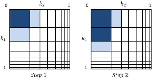
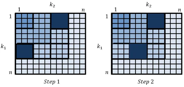
Fig. 2. Geometric representation of the rst two steps of key enumeration.
successors of this candidate: (k1(j1+1), k(2j2)) and (k1(j1), k(2j2+1)). An important
observation made by [20] is that F should never include 2 candidates in the
same column, or in the same row: one candidate will clearly dominate the other. Thus the algorithm maintains auxiliary data structures (bit vectors) to indi-cate which rows and columns currently have member inF. This observation has
a crucial eect on the size of the data structure,|F|.
We can see in Figure 2 the rst steps of the algorithm: the most likely key is (k1(1), k2(1)), therefore this is the key that is output rst (represented in dark
gray in step 1). Now, the only possible next key candidates are the successors (represented in light gray in step 1)(k(2)1 , k(1)2 )and(k(1)1 , k(2)2 ), which are inserted
into F. Then again, the most likely key is extracted, but this time only one
successor is inserted because there is already a key in column2.
In general the number of dimensionsd >2 and we need to enumerate over
more than two lists of subkeys. For AES, typically d = 16 for byte-level side
channels or d = 4 for 32-bit subkeys as in [15]. To do this, [20] suggested a
recursive decomposition of the problem. The algorithm described above is only used for merging two lists, and its outputs are used to form larger subkey lists which are in turn merged together. In order to minimize the storage and the enumeration eort, these lists are generated only as far as required by the key enumeration. Therefore, whenever a new subkey is inserted into the candidate set, its value is obtained by applying the enumeration algorithm to the lower level, (for example 64-bit subkeys obtained by merging two 32-bit subkeys), and so on.
3 Bounding the Guessing Entropy
keys to test before reaching the correct one, based on the probabilities assigned to key candidates by the side channel attack.
Denition 1 (Guessing Entropy). For a random variable X with n values,
denote the elements of its probability distributionPX byPX(xi)forxi∈X such
that PX(x1)≥PX(x2)≥...≥PX(xn). The guessing entropy ofX is:
G(X) = n X
i=1
i·PX(xi).
The cased= 2: Let the key be split into 2 independent subkey spaces X and Y,
each of size n, thus a key is a vector xys.t. x∈X andy ∈ Y. A side channel
attack produces 2 separate distributions PX(xi) for xi ∈ X and PY(yj) for
yj ∈Y. Assume that the subkey distributions are sorted:PX(x1)≥PX(x2)≥
...≥PX(xn)and similarly forPY, thenG(X)andG(Y)are well dened.
Let XY denote the list of (full) keys sorted in decreasing order of
proba-bility, where PXY(xi, yj) = PX(xi)PY(yj) since the subkeys are independent.
ThusG(XY)is well dened. However, calculatingG(XY) requires a time and
space complexity ofΩ(n2). Therefore boundingG(XY)in terms of the easy-to-compute G(X)and G(Y)is a useful goal. To this end, let rank(xi, yj) be the
position of key(xi, yj)inXY. Clearly,rank(x1, y1) = 1andrank(xn, yn) =n2.
By denition we get:
G(XY) = n X
i=1
n X
j=1
rank(xi, yj)·PX(xi)PY(yj). (1)
Theorem 1. The guessing entropy of XY,G(XY), is bounded by:
G(X)G(Y)≤G(XY)≤n(G(X) +G(Y))−G(X)G(Y). (2)
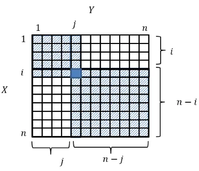
Proof. As mentioned in [21], and as depicted in Figure 3 given a key(xi, yj), all
the key candidates with higher indexes in both indexes, have a lower probability and higher rank, and all the key candidates with lower indexes, have a lower rank.
Taking advantage of this fact,rank(xi, yj)can be bounded as follows:
Fig. 3. Another geometric representation of the key space
We use this observation in order to boundG(XY). First, we prove the lower
bound. By substituting Eq. (3) in Eq. (1) we get:
G(XY) = n X
i=1
n X
j=1
rank(xi, yj)·PX(xi)PY(yj)
≥
n X
i=1
n X
j=1
ij·PX(xi)PY(yj)
= n X
i=1
i·PX(xi) n X
j=1
j·PY(yj)
=G(X)G(Y).
Second, we prove the upper bound ofG(XY). By Eq. (3),
By substituting Eq. (3) in Eq. (1) we get:
G(XY) = n X i=1 n X j=1
rank(xi, yj)·PX(xi)PY(yj)
≤ n X i=1 n X j=1
n(i+j)−ij
·PX(xi)PY(yi)
=n n X i=1 n X j=1
(i+j)·PX(xi)PY(yj)− n X i=1 n X j=1
ij·PX(xi)PY(yj)
=n n X i=1 n X j=1
(i+j)·PX(xi)PY(yj)−G(X)G(Y). (*)
We calculate separately the summation at Eq. (*),
n X i=1 n X j=1
(i+j)·PX(xi)PY(yj) = n X
i=1
PX(xi) n X
j=1
(i+j)·PY(yj)
= n X
i=1
PX(xi) hXn
j=1
i·PY(yi) + n X
j=1
j·PY(yj) i
= n X
i=1
i·PX(xi) n X
j=1
PY(yj)
| {z }
1
+ n X
j=1
PX(xi) n X
j=1
j·PY(yi)
| {z }
G(Y)
=G(X) +G(Y).
By substituting the results in Eq. (*) we get:
G(XY) =n G(X) +G(Y)
−G(X)G(Y) (4)
Which concludes the proof of the theorem. We can see that in general G(XY)
is not multiplicative:
Corollary 1 G(X)G(Y)≤G(XY)≤2n·max G(X), G(Y).
Proof. Without loss of generality, we assume that G(X) ≥ G(Y) ≥ 1 then
Eq. (4) can be bounded by:
G(XY)≤n·2G(X)−G(X) = (2n−1)G(X)≤2n·max G(X), G(Y)
.
These bounds can be expanded ford >2. In this case it holds: d
Y
m=1
im≤rank(x
(1)
i1 , x (2)
i2 , ..., x (d)
id )≤n
d
−
d Y
m=1
Therefore we obtain
Theorem 2. The guessing entropyG(X(1)X(2)...X(d)), is bounded by: d
Y
m=1
G(X(m))≤G(X(1)X(2)...X(d))≤nd−
d Y
m=1
(n−G(X(m))).
As an example of using these bounds, with byte-level SCA on AES we have
d = 16. If the SCA discards 128 values per byte and returns a probability
distribution over the remaining 128 candidates we haven= 128. Assuming that
G(X(m)) = 8for all 16 subkeys we get that
248= 816≤G(X(1)X(2)...X(d))≤12816−(128−8)16= 2111.36.
Note that the upper bound is rather weak, especially whenG(X)is lowwhich
is usually the case in successful SCA scenarios.
4 Key Enumeration algorithm
The key enumeration in [20] enumerates the key candidates in optimal order, but has a signicant drawback, its memory requirements may exceed the available memory. Its worst-case space complexity isΩ(nd/2)since it needs to store the full sorted distribution of the 2 top-level dimensions (in addition to the data structure
F). Moreover, in order to enumerate until a key of rankr≤nd/2 it has a space
complexity ofΩ(r). In this section, we present a new key enumeration algorithm
with bounded memory requirements, which therefore allows to enumerate a large number of key candidates.
To achieve the desired memory bound, we relax the optimal order require-ment: our algorithm enumerates the keys in near-optimal order, and we are able to bound the ratio between the optimal rank of a key and our algorithm's rank of that key.
4.1 The layering approach
In order to explain our algorithm, we start with the cased= 2. We divide the
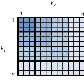
key-space into layers of widthw, as depicted in Figure 4. The rst layer contains the
keys(k(1i), k(2j))such that(i, j)∈ {1, ..., w}×{1, ..., w}. The second layer contains the keys(k1(i), k2(j))such that(i, j)∈ {1, ...,2w}×{1, ...,2w}\{1, ..., w}×{1, ..., w} and so on. More formally:
Denition 2. Given w >0 andl >0, let
layerlw={(k
(i) 1 , k
(j)
2 )|(i, j)∈ {1, ..., l·w}×{1, ..., l·w}\{1, ...,(l−1)·w}×{1, ...,(l−1)·w}}. A key observation is that we can run the optimal enumeration algorithm of [20] within a layer: we seed the algorithm data structureF by inserting the two
Fig. 4. Geometric representation of the key space divided into layers of widthw= 3. The keys in cells(1,7)and(7,1)are the algorithm's seeds forlayer(3)3
Proposition 1. For every l >0 andw >0, applying the optimal key
enumer-ation of [20] on layerw
l , the number of next potential key candidates is bounded
by 2w, i.e., |F| ≤2w.
Proof. The proof is directly derived from the key enumeration algorithm [20]. The algorithm extracts the highest probability key candidate from the data structureF, and inserts its successors intoF, while keeping the rule thatFmay
contain at most one element in each row and column oflayerwl . Looking at the
geometrical representation,layerlw is a union of a horizontal rectangleHlw and
a vertical rectangleVlw, such that
Hlw={(k1(i), k2(j))∈layerwl |(l−1)·w < i≤l·w},
Vlw={(k1(i), k(2j))∈layerwl |(l−1)·w < j≤l·w}.
layerwl =Hlw∪Vlw.
Therefore, the size ofF, for every layerwl is:
|F| ≤ |F∩Hlw|+|F∩Vlw|
Because F may contain at most one element in each column and row, the
size of|F∩Hlw|is the minimum between Hlw's two dimensions:
|F∩Hlw| ≤min{w, l·w}=w,
and similarly for|F∩Vw
l |. Therefore, we get
|F| ≤2w.
Importantly, the bound on|F|is independent ofn, and depends only on the
Fig. 5. Geometric representation of the key space divided into squares of widthw= 3.
4.2 The Two-Dimensional Algorithm
Proposition 1 leads us to our w-layer key enumeration algorithm: Divide the
key-space into layers of width w. Then, go over the layerws, one by one, in
increasing order. For eachlayerlw, enumerate its key candidates, by applying the
optimal key enumeration [20]. Following the proposition, the number of potential next candidates,F, that our algorithm should store is bounded by2w.
Ford= 2, the sorted orders of keys in the 2 subkey spaces are given
explic-itly. However, for d >2 during the recursive descent, we need to generate the
ordered lists on the y as far as required. We do this by applying a recursive de-composition of the problem. The length of these generated subkey spaces grows and eventually becomes too large to store. Therefore, instead of naively storing the full subkey order, we only store theO(w)candidates which were computed
recently.
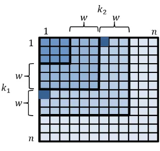
To do this, we divide each layerw in the geometrical representation, into
squares of size w×w, as depicted in Figure 5. Our algorithm still enumerates
the key candidates inlayerw
1 rst, then inlayer2wand so on, but in eachlayerwl
the enumeration will be square-by-square. More specically, letSw
x,y be a set of the key candidates in the squareSwx,y=
{(k1(i), k2(j))|(x−1)·w < i ≤x·wand(y−1)·w < j ≤ y·w}. We say that two squares, Sx,y andSz,w are in the same rowify=w, and are in the same
columnifx=z.
Now let's describe the enumeration at eachlayerw
l . We know that the most
likely candidate inlayerw
l is either atS1,l orSl,1. Therefore, we enumerate rst
the key candidates inS1,l∪Sl,1by applying the key enumeration in [20] on them (represented in dark gray in step 1 in Figure 6). LetS denote the set of squares
that contain potential next candidates in this layer. At some point, one of the two squares is completely enumerated. Without loss of generality, we assume this isS1,l. At this point, the only square that contains the next key candidates
Fig. 6. Geometric representation of the key enumeration atlayer33.
In general case, the successor ofSx,y is eitherSx+1,y orSx,y+1, only one of
which is inlayerwl . Therefore, when one of the squares is completely enumerated,
it is extracted fromS, and its successor is inserted, as long asS doesn't contain
a square in the same row or column.
Notice that only after a square is completed we continue to it's successor. Without loose of generality, we assume that the successor is in the same row as the current one. Therefore, for all candidates(k1(i), k2(j))we intend to check next,
the j index is higher than thej index of any candidate in the current square,
therefore thesej indexes of the current square are useless hence are not stored.
It is simple to see thatScontains at most2squares of sizew×weach step,
therefore only the subkeys at each dimension should be stored, which means a space complexity ofO(w).
4.3 Generalization to multi-dimensional Algorithm
Similarly to [20] we apply a recursive decomposition of the problem. Whenever a new subkey is inserted into the candidate set, its value is obtained by applying the enumeration algorithm to the lower level, (for example 64-bit subkeys obtained by merging two 32-bit subkeys). For example, let's look at d = 4. In order to
generate the ordered full-key, we need to generate the 2 ordered lists of the lower level on the y as far as required. In the worst case the space complexity of these 2 lists is Ω(n2). Although the size of the data structure F is bounded by 2w, we still have a bottleneck ofΩ(n2). Therefore, instead of naively storing the full subkey order, we only store theO(w)candidates which computed recently. We
store2wsubkeys of the rst low-level list, and another2wsubkeys of the second
Algorithm 1: w-Layer Key Enumeration Algorithm. Input: Subkey distributions{ki}1≤i≤d.
Output: The correct key, if exists, NOT-FOUND otherwise. 1 currentLayer= 1;
2 f ound=f alse;
3 while (currentLayeris not out of range) do
4 S←S1,currentLayer∪ScurrentLayer,1;
5 while (S6=∅) do
6 candidate= nextCandidate(S,{ki}1≤i≤d);
7 f ound= isCorrectKey(candidate);
8 if (f ound) then
9 returncandidate;
10 end
11 end
12 currentLayer+ + 13 end
14 return NOT-FOUND;
4.4 Bounding the Rank and the Guessing Entropy
Let vw denote the vector resulting from enumerating all key candidates,
ap-plying our w-layer key enumeration, for xed w, and let v denote the
vec-tor resulting from applying the optimal order enumeration. Additionally, let
rankw(i1, i2, .., id) denote the order statistic of key(k
(i1) 1 , k
(i2) 2 , ..., k
(id)
d ) in v w,
andrank(i1, i2, .., id)be the order statistic of key(k
(i1) 1 , k
(i2) 2 , ..., k
(id)
d )inv. Now,
we want to bound the rank of thew-layer algorithm, and the guessing entropy
ofvw,G(vw), related toG(v).
Theorem 3. Consider a key (k(1i1), ..., k(id)
d ). Let i
∗ = max{i
1, ..., id}, and let
αm=im/i∗ form= 1, ..., d(αm≤1). Then,
rankw(i1, ..., id)≤ d Y m=1 2 αm
·rank(i1, ...,1d).
Proof. According Eq. (3), it holds that:
rank(i1, i2, ..., id)≥ d Y
m=1
im.
Without loss of generality, we assume that the maximal indexi∗=i1. Using
that, we get:
rank(i1, i2, ..., id)≥ d Y
m=1
im=id1·
d Y
m=1
αm. (5)
Our goal is to upper-boundrankw(i
1, i2, .., id). We divide the analysis into
Algorithm 2: nextCandidate.
Input: Set of squares with potential candidatesS and Subkey distributions {ki}1≤i≤d.
Output: The next key candidat inS.
1 main,{1, ..., d};
2 x,{1, ..., d/2};
3 y,{d/2 + 1, ..., d};
4 (kx(i), ky(j))←most likely candidate inFmain; 5 F1,d←F1,d\ {(kx(i), ky(j))};
6 Si,j←the square which(kx(i), k(yj))is inside; 7 if Si,j is completely enumerated then 8 S←S\Si,j;
9 if no square in same row/column asSuccessor(Si,j)then 10 S←S∪Successor(Si,j);
11 Fmain←Fmain∪ {most likely candidate inSuccessor(Si,j)}; 12 end
13 else
14 if (k(xi+1), k
(j)
y )∈S and no candidate in row i+1 then 15 if kx(i+1) hasn't calculated yet then
16 nextCandidate({ki}i∈x);
17 k(xi+1)←the most likely candidate inFx;
18 end
19 Fmain←Fmain∪ {(k
(i+1)
x , k
(j)
y )}; 20 end
21 if (k(xi), k(yj+1))∈S and no candidate in column j+1 then 22 if ky(j+1) hasn't calculated yet then
23 nextCandidate({ki}i∈x);
24 k(yj+1)←the most likely candidate inFy;
25 end
26 Fmain←Fmain∪ {(kx(i), k(yj+1))}; 27 end
28 end
Fig. 7. Geometric representation of key(k(i1) 1 , k
(i2)
2 )atlayer 3
2 withi1= 8,i2= 3and
w= 3.
case 1:i1≥w. In this case, the key(k (i1) 1 , k
(i2) 2 , ..., k
(id)
d )is at somelayer w l such
thatl >1. According to ourw-layer key enumeration, we enumerate all the keys
in the current layer, before we continue to the next layer. Therefore, the rank of this key is bounded by the total number of keys in layers 1, .., l. As we can
see in Figure 7, for the bi-dimensional case, the distance between i1 and the high bound of the layer l is at most w. Since i1 was maximal, the high bound of the layer l is at most i1+w for all ddimensions, and rankw(i1, i2, ..., id) is
upper-bound by
rankw(i1, i2, ..., id)≤(i1+w)d. (6) Using our assumption thati1≥w, we get:
(i1+w)d ≤(2·i1)d= 2d·id1. (7) Plugging Eq. (6) and Eq. (7) into Eq. (5) yields
rankw(i1, i2, ..., id)≤ d Y
m=1
2
αm
·rank(i1, i2, ..., id).
case 2: i1 < w. In this case, the key (k (i1) 1 , k
(i2) 2 , ..., k
(id)
d ) is at the rst layer
layer1w. Therefore, our w-layer key enumeration, enumerates the keys in the same order the optimal key enumeration does, possibly skipping the keys which are outside this layer. Therefore:
rankw(i1, i2, ..., id)≤rank(i1, i2, ..., id)
and in particular,
rankw(i1, i2, ..., id)≤ d Y
m=1
2
αm
since 2
αm >1for allm.
Theorem 4. The boundary of the guessing entropy of vw, G(vw), related to
G(v) is:
G(vw)≤2dnd−1·G(v).
Proof. Each subkey contains n values, therefore, i1 is at most n times bigger than any ofi2, ..., id, means for eachm∈ {2, ..., d},αm≥1/n. Applying this on
Theorem 3, we get:
rankw(i1, i2, ..., id)≤2d·nd−1·rank(i1, i2, ..., id).
Therefore,
G(vw)≤2d·nd−1·G(v).
4.5 Space Complexity Analysis
The algorithm needs to store for each level a list, of sizew, of subkeys obtained
from applying the algorithm on lower level. For this, it needs to store 2 squares of sizew×wfor the 2 top-level dimensions, which means 4 lists. In addition, it
needs to store, for the current level, a data structureF which bounded by2wand
2 data structures (bit vectors) to indicate which rows and columns currently have member inF. Totally we get the following space recurrence relation:
S(d) = 4S(d/2) +cw,
for some constantc, which sums toO(d2w). Taking into account the input, whose
space isO(dn), we get a total space complexity ofO(d2w+dn).
5 Modeling the subkey probability distribution
Probabilistic side channel attacks such as template attacks [7] produce a proba-bility distribution for each subkey, interpreted as the probaproba-bility that a particular subkey value is correct. However, with data sets such as the DPAv4 [1] we know the true correct keys over traces from many dierent keys. Hence, it is possible to compare to SCA-predicted probability distribution with reality.
Assuming that the SCA-distribution PXk for a subkey X on key instance k, is sorted in decreasing order, hence PXk(xi)is the SCA probability that the
correct key of instance k has rank i. However, we also know the true rank r∗
of the correct key for each instance k, according to the order implied by Pk X.
Thus we can calculate the true rank probability distribution: let P∗
X(r)be the
frequency of subkey instances such that the subkey at position r according to
the SCA-order is the correct subkey.
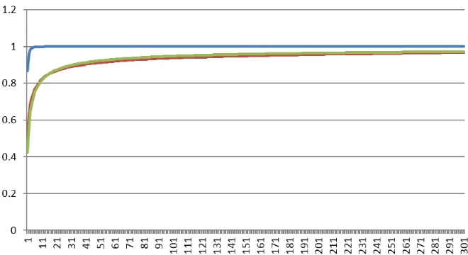
Figure 8 shows the SCA-predicted probability distribution versus the true rank distribution, using the data of Oren, Weisse and Wool in [15].
Fig. 8. The cdf of the average SCApredicted probability distribution (top curve -blue), the true empirical rank probability distribution PX∗ (red) and the synthetic Pareto distribution (green) as function of the rank. Note that the cdf curves for the empirical and synthetic distributions overlap almost completely.
guessing entropy, with G(X) = 1.2 to the SCA-predicted compared to 135 for
the true rank probability distribution.
We can see that the true distribution has a long tail: large ranks do appear with non-negligible probability. A good distribution which models long-tail dis-tributions is the Pareto Distribution [3]. If X is a random variable with a Pareto distribution, then the PDF is given by:
fX(x) =
α
xα+1, forx≥1.
In order to simulate the true rank distribution, we choose parameters that lead the expected value to equal the guessing entropy of the rank distribution, 135, by solving the following equations:
β
n X
x=1
fX(x) =β· n X
i=1
α xα+1 = 1 and
E(X) =β
n X
x=1
x·fX(x) =β n X
x=1
α
xα = 135.
Ford= 4and n= 217 (as in the results of [15]), we obtainα= 0.575, and
β = 0.738. Figure 8 also shows a curve for this Pareto distribution demonstrating
This observation leads to two conclusions. First, it shows that, at least for the method of [15], the SCA-predicted distribution and the claimed guessing entropy are overly optimistic - it would be interesting to evaluate other SCA attacks using this methodology. Second, using Pareto distributions as a model we can simulate various scenarios for the key enumeration algorithms without creating an actual SCA attack.
6 Performance Analysis
We evaluated the performance of ourw-layer key enumeration algorithm through
an extensive simulation study. We implemented the optimal algorithm [20] and our algorithm in Java, and ran both algorithms on a 3.07GHz PC with 24GB RAM running Microsoft windows 7, 64bit. Note that the code of the optimal algorithm is used as a subroutine in the w-layer algorithm, thus any potential
improvement in the former's implementation would automatically translate into an analogous improvement in the latter.
We used synthetic SCA distributions withd= 8dimensions andn= 212for a total enumeration space of296. The 8 probability distributions were generated according to the model of Section 5: Pareto distributions tting G(X) = 135,
with α = 0.575 and β = 0.738. We analyzed our w-layer algorithm for two
dierent values of w:(i)w=n= 212 and(ii)w= 225.
We also evaluated the algorithm's performance ford= 16dimensions andn= 26, again for a total enumeration space of296. The 16 probability distributions
were Pareto distributions tting G(X) = 8, with α= 0.3 andβ = 1.1197. We
analyzed ourw-layer algorithm for two dierent values ofw:(i)w=n= 26and (ii) w= 225. The obtained results are similar to those with d= 8. Graphs are omitted.
We conducted the experiments as follows. We ran the optimal algorithm on dierent (optimal) ranks starting from 212, and measured its time and space consumption. For each optimal rank,2x, we extracted the key corresponding to
this rank, and ran each of ourw-layer key enumeration algorithm variants until
it reached the same key, and measured its rank, time and space. We repeated this simulation for 64 dierent ranks near 2x the graphs below display the
median of the measured values.
6.1 Runtime Analysis
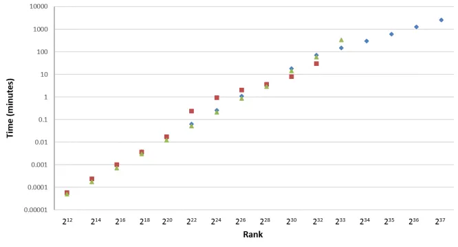
Figure 9 illustrates the time (in minutes) of the 3 algorithms: optimal-order (green triangles), w-layer with w =n (red squares) and w-layer with w = 225 (blue diamonds) for dierent ranks. The gure shows that, crucially, the optimal-order key enumeration stops at233. This is because of high memory consumption which exceeds the available memory.
For ranks beyond222we noticed that thew-layer enumeration withw=n=
Fig. 9. Time, in minutes, of optimal-order key enumeration (green triangles),w-layer
key enumeration with w = 225 (blue diamonds) and w-layer key enumeration with
w=n(red squares) on dierent ranks.
at the 2 hour mark, and we stopped experimenting with this setting beyond rank232. It is important to remark that we chose to stop because of the time consumption - the algorithm doesn't stop till it gets to the correct key.
For thew-layer withw= 225 we can see excellent results. For small ranks it takes exactly the same time consumption as the optimal-order, (hidden by the green triangles in Figure 9), and for high ranks, its bounded space complexity enables it to enumerate in reasonable time.
Note that for ranks beyond233, the optimal algorithm failed to run, so we could not identify the keys with those ranks. In order ro demonstrate thew-layer
algorithm's ability to continue its enumeration we let it run until it reached a rank
rin its own near-optimal order (forr= 234, ..,237) - and for those experiments we removed the 2 hour time out.
6.2 Space Utilization
Figure 11 illustrates the space (in bytes) used by the 3 algorithms' data structures for dierent ranks. As we can see again, the optimal-order key enumeration stops at 233 because memory shortage. For thew-layer algorithm withw=nwe can clearly see the bounded space consumption leveling at around 1MB. For thew
Fig. 10. Frequency of the keys whose time consumption applying thew-layer key
enu-meration withw=nis higher than 2 hours.
6.3 The Dierence in Ranks
Figure 12 illustrates the ranks detected by the 3 algorithms as a function of the optimal rank. By denition the optimal algorithm nds the correct ranks. Despite the somewhat pessimistic bounds of Theorem 4, the gure shows that with w =n the ratio between the optimal rank are rankw is approximately 5
(again, beyond228 too many runs timed out for meaningful data). Forw= 225 the discovered ranks are almost identical to the optimal ranks (the symbols in the gure overlap) - and beyond233the optimal algorithm failed so comparison is not possible.
7 Conclusion
In this paper, we investigated the side channel attack improvement obtained by adversaries with non-negligible computation power to exploit physical leakage. For this purpose, we presented a new w-layer key enumeration algorithm that
trades-o the optimal enumeration order in favor of a bounded memory con-sumption. We analyzed the algorithm's space complexity, guessing entropy, and rank distribution. We also evaluated its performance by extensive simulations. As our simulations show, ourw-layer key enumeration allows stronger attacks than
Fig. 11. Space, counting the data structure elements, of optimal-order key enumeration (green triangles),w-layer key enumeration withw= 225(blue diamonds) andw-layer
key enumeration withw=n(red squares) on dierent ranks.
Along the way we provided bounds on the full key guessing entropy in terms of the guessing entropies of the individual subkeys. We also observed a signicant gap between the predicted and the true rank distributions of a real SCAwe showed that the true rank distribution is long-tailed, and well modeled by a Pareto distribution.
Finally, an open-source Java implementation for both ourw-layer key
enu-meration and the order-optimal enuenu-meration [20] are available via the authors' home pages.
References
1. DPA contest v4. http://www.dpacontest.org/v4/.
2. Dakshi Agrawal, Bruce Archambeault, Josyula R Rao, and Pankaj Rohatgi. The EM side-channel (s). In Cryptographic Hardware and Embedded Systems-CHES 2002, pages 2945. Springer, 2003.
3. Barry C Arnold. Pareto distribution. Wiley Online Library, 1985.
4. Daniel J Bernstein, Tanja Lange, and Christine van Vredendaal. Tighter, faster, simpler side-channel security evaluations beyond computing power. Cryptology ePrint Archive, Report 2015/221, 2015. http://eprint.iacr.org/.
Fig. 12. Rank of optimal-order key enumeration (green triangles), w-layer key
enu-meration withw= 225(blue diamonds) andw-layer key enumeration withw=n(red
squares) on dierent ranks.
6. Eric Brier, Christophe Clavier, and Francis Olivier. Correlation power analysis with a leakage model. In Cryptographic Hardware and Embedded Systems-CHES 2004, pages 1629. Springer, 2004.
7. Suresh Chari, Josyula R Rao, and Pankaj Rohatgi. Template attacks. In Cryp-tographic Hardware and Embedded Systems-CHES 2002, pages 1328. Springer, 2003.
8. Markus Dichtl. A new method of black box power analysis and a fast algorithm for optimal key search. Journal of Cryptographic Engineering, 1(4):255264, 2011. 9. Karine Gandol, Christophe Mourtel, and Francis Olivier. Electromagnetic anal-ysis: Concrete results. In Cryptographic Hardware and Embedded SystemsCHES 2001, pages 251261. Springer, 2001.
10. Pascal Junod and Serge Vaudenay. Optimal key ranking procedures in a statistical cryptanalysis. In Fast Software Encryption, pages 235246. Springer, 2003. 11. Paul Kocher, Joshua Jae, and Benjamin Jun. Dierential power analysis. In
Advances in CryptologyCRYPTO'99, pages 388397. Springer, 1999.
12. Paul C Kocher. Timing attacks on implementations of die-hellman, rsa, dss, and other systems. In Advances in CryptologyCRYPTO'96, pages 104113. Springer, 1996.
13. Daniel P. Martin, Jonathan F. O'Connell, Elisabeth Oswald, and Martijn Stam. Counting keys in parallel after a side channel attack. In Advances in Cryptology ASIACRYPT 2015, pages 313337. Springer, 2015.
15. Yossef Oren, Or Weisse, and Avishai Wool. A new framework for constraint-based probabilistic template side channel attacks. In Cryptographic Hardware and Embedded SystemsCHES 2014, pages 1734. Springer, 2014.
16. Jing Pan, Jasper GJ Van Woudenberg, Jerry I Den Hartog, and Marc F Witteman. Improving DPA by peak distribution analysis. In Selected Areas in Cryptography (SAC), pages 241261. Springer, 2011.
17. Romain Poussier, Vincent Grosso, and François-Xavier Standaert. Comparing ap-proaches to rank estimation for side-channel security evaluations. In Smart Card Research and Advanced Applications (CARDIS). Springer, 2015.
18. Jean-Jacques Quisquater and David Samyde. Electromagnetic analysis (EMA): Measures and counter-measures for smart cards. In Smart Card Programming and Security, pages 200210. Springer, 2001.
19. François-Xavier Standaert, Tal G Malkin, and Moti Yung. A unied framework for the analysis of side-channel key recovery attacks. In Advances in Cryptology-EUROCRYPT 2009, pages 443461. Springer, 2009.
20. Nicolas Veyrat-Charvillon, Benoît Gérard, Mathieu Renauld, and François-Xavier Standaert. An optimal key enumeration algorithm and its application to side-channel attacks. In Selected Areas in Cryptography (SAC), pages 390406. Springer, 2013.
21. Nicolas Veyrat-Charvillon, Benoît Gérard, and François-Xavier Standaert. Security evaluations beyond computing power. In Advances in CryptologyEUROCRYPT 2013, pages 126141. Springer, 2013.