Adaptive Random Testing Based on
Distribution Metrics
∗
Tsong Yueh Chen, Fei-Ching Kuo, Huai Liu
†Faculty of Information and Communication Technologies
Swinburne University of Technology
John Street, Hawthorn 3122 Victoria, Australia
Abstract
Random testing (RT) is a fundamental software testing technique.
Adaptive random testing(ART), an enhancement of RT, generally uses fewer test cases than RT to detect the first failure. ART generates test cases in a random manner, together with additional test case selection criteria to enforce that the executed test cases are evenly spread over the input domain. Some studies have been conducted to measure how evenly an ART algorithm can spread its test cases with respect to some distribution metrics. These studies observed that there exists a correlation between the failure detection capability and the evenness of test case distribution. Inspired by this observation, we aim to study whether failure detection capability of ART can be
∗A preliminary version of this paper was presented at the 7th International Conference
on Quality Software (QSIC 2007) (Chen et al., 2007a).
†Corresponding author. Tel.: +61 3 9214 5276; fax: +61 3 9819 0823.
enhanced by using distribution metrics as criteria for the test case selection process. Our simulations and empirical results show that the newly proposed algorithms not only improve the evenness of test case distribution, but also enhance the failure detection capability of ART.
Keywords: Software Testing, Random Testing, Adaptive Ran-dom Testing, Test Case Distribution, Discrepancy, Dispersion.
1
Introduction
Improving software quality has become one of the important objectives for
the current software industry (NIST, 2002). Software testing, a major
ap-proach to software quality assurance (Hailpern and Santhanam, 2002), is
widely acknowledged as a vital activity throughout the software
develop-ment process. Many software testing methods are accomplished by
defin-ing test objectives, selectdefin-ing some inputs of the program under test as test cases, executing the program with these test cases, and analysing testing results (Beizer, 1990). Since software normally has an extremely largeinput domain (that is, the set of all possible program inputs), testers are always re-quired to select a portion of the input domain as test cases such that software
failures can be effectively detected with this selected portion of test cases. A
large number of software testing methods have been proposed to guide the
test case selection.
Random testing (RT), a basic test case selection method, simply selects test cases in a random manner from the whole input domain (Hamlet, 2002;
Myers, 2004). RT has been popularly applied to assess the software
reliabil-ity (Girard and Rault, 1973; Thayer et al., 1978). In addition, RT has been
(1990, 1995) have used RT to test UNIX utility programs, and reported that
a large number of UNIX programs have been crashed or hanged by RT.
For-rester and Miller (2000) applied RT to test Windows NT applications, and it
was observed that 21% of applications were crashed and an additional 24%
of applications were hanged. RT has also been used in the testing of
com-munications protocol implementations (West and Tosi, 1995), graphical user
interfaces (Dab´oczi et al., 2003), Java Just-In-Time compilers (Yoshikawa
et al., 2003), embedded software systems (Regehr, 2005), and image
process-ing applications (Mayer and Guderlie, 2006). Moreover, the RT technique
has been implemented in many industrial automatic testing tools, such as
those developed by IBM (Bird and Munoz, 1983), Microsoft (Slutz, 1998),
and Bell Labs (Godefroid et al., 2005).
However, some people (Myers, 2004) criticised that RT may be the “least
effective” testing method for using little or no information about the
pro-gram under test to guide its test case selection. One common characteristic
of faulty programs is that thefailure-causing inputs (program inputs that can reveal failures) are usually clustered together, as reported by White and
Co-hen (1980), Ammann and Knight (1988), Finelli (1991), and Bishop (1993).
Chen et al. (2004) investigated how to improve the failure detection
capabil-ity of RT under such a situation. Given that failure-causing inputs tend to
cluster into contiguous regions (namelyfailure regions (Ammann and Knight, 1988)), non-failure regions are also contiguous. Therefore, if a test case does
not reveal any failure, it is very likely that its neighbours would not reveal a
failure either. In other words, given the same number of test cases, a more
even spread of test cases should have a better chance to detect a failure.
When RT is used to detect software failures, inputs are usually selected as
probability of being selected as test cases. Therefore, an input that is
adja-cent to some previously executed but non-failure-causing test cases may still
be selected as the next test case. However, such a test case is also unlikely
to reveal failure. Aiming at enhancing the failure detection capability of RT,
Chen et al. (2004) proposed a new approach, namely adaptive random test-ing (ART). Like RT, ART also randomly generates test cases from the input domain. But ART uses additional criteria to guide the test case selection
in order to ensure that all test cases are evenly spread over the whole input
domain. Different test case selection criteria give rise to different ART al-gorithms, such as fixed-sized-candidate-set ART (FSCS-ART) (Chen et al., 2004),lattice-based ART (Mayer, 2005), andrestricted random testing (Chan et al., 2006). Previous simulations and empirical studies conducted on these
algorithms have shown that in general, when failure-causing inputs are
clus-tered into contiguous failure regions, ART uses fewer test cases to detect the
first failure than pure RT.
Chen et al. (2007b) have used several metrics to measure and compare
the test case distributions of various ART algorithms. Among these metrics,
discrepancy and dispersion are two metrics commonly used to measure the equidistribution of sample points. Chen et al. (2007b) investigated both the
test case distributions and the failure detection capabilities of some ART
algorithms, and they empirically justified that there exists a correlation
be-tween the test case distribution and the failure detection capability of an
ART algorithm. For example, the test case selection criterion in FSCS-ART
may bring a large value of discrepancy when the dimension of input domain
is high; while the failure detection capability of FSCS-ART becomes worse
as the dimension of input domain increases.
test cases is correlated to a high failure detection capability. Since
discrep-ancy and dispersion reflect different aspects of the test case distribution, we
are motivated to apply these metrics as criteria in the test case selection
pro-cess of ART, aiming at improving the evenness of test case distribution and
the failure detection capability of ART. However, adopting distribution
met-rics as the new test case selection criteria of ART is not so straightforward as
it looks. As will be shown in our study, if an ART algorithm applies
discrep-ancy or dispersion as the standalone test case selection criterion, it will have
an uneven distribution of test cases as well as a poor failure detection
capa-bility. In this paper, we also investigate whether the performance of ART
can be enhanced if discrepancy and dispersion are integrated with existing
test case selection criteria. Our study delivers some interesting results.
Our work is conducted on a particular ART algorithm, namely
FSCS-ART. The structure of the paper is as follows. In Section 2, we give some
preliminary background of ART and present the basic concepts of discrepancy
and dispersion. We propose two new test case selection criteria based on
discrepancy and dispersion in Section 3. In Section 4, we investigate the
performance of ART algorithms that solely use discrepancy or dispersion to
select test cases. In Section 5, we propose some new ART algorithms where
discrepancy and dispersion are integrated with other criteria in the test case
selection process. The simulations and experimental results of these new
algorithms will also be reported in this section. Finally, Section 6 presents
2
Background
2.1
Notation
For ease of discussion, we introduce the following notation, which will be
used in the rest of this paper.
• E denotes the set of already executed test cases.
• I denotes the input domain.
• dI denotes the dimension ofI, which is the number of input parameters of the program under test.
• ND denotes N-dimension, where N = 1, 2,· · ·, dI.
• | · | denotes the size of a set. For example, |E| and |I| denote the size
of E and I, respectively.
• dist(p, q) denotes the Euclidean distance between two pointsp and q.
• η(p, E) denotes p’s nearest neighbour inE.
2.2
One test case selection criterion of adaptive
ran-dom testing
Generally speaking, besides randomly generating program inputs, ART uses
additional criteria to select inputs as test cases in order to ensure an even
spread of test cases. Fixed-sized-candidate-set ART (FSCS-ART) (Chen et al., 2004) is one typical ART algorithm. In FSCS-ART, there exist two
not reveal any failure; while C contains k randomly generated inputs, where
k is fixed throughout the testing process. The test case selection criterion of
FSCS-ART is as follows. For any cj ∈C, we define
djdistance =dist(cj, η(cj, E)). (1)
We choose a candidatecb as the next test case, if itsdbdistance is the largest amongst all candidates, that is,∀j = 1,2,· · · , k, db
distance≥d j
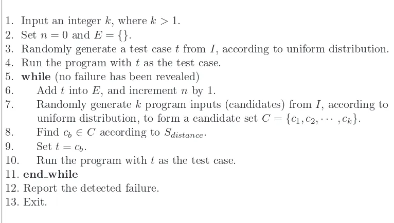
distance. The test case selection criterion of FSCS-ART is referred to as Sdistance in this paper. Figure 1 gives the detailed algorithm of FSCS-ART. Chen et al. (2004)
have observed that the effectiveness of FSCS-ART can be significantly
im-proved by increasing k when k ≤ 10. However, the effectiveness appears to
be independent of the value of k when k > 10. In other words, k = 10 is
close to the optimal setting of FSCS-ART. Hence, they have used k = 10 in
their investigation. In this paper, we also set the default value of k as 10.
1. Input an integer k, wherek >1. 2. Set n= 0 andE ={}.
3. Randomly generate a test case tfrom I, according to uniform distribution. 4. Run the program with tas the test case.
5. while (no failure has been revealed) 6. AddtintoE, and increment nby 1.
7. Randomly generatek program inputs (candidates) fromI, according to uniform distribution, to form a candidate set C={c1, c2,· · · , ck}.
8. Find cb ∈C according to Sdistance.
9. Sett=cb.
10. Run the program with tas the test case. 11. end while
12. Report the detected failure. 13. Exit.
Figure 1: The algorithm of FSCS-ART
that the program under test only has numeric inputs. Applications of ART
on non-numeric programs can be found in the studies of Merkel (2004), Kuo
(2006) and Ciupa et al. (2006, 2008).
2.3
Failure detection capability of adaptive random
testing
F-measure, one commonly-used metric for measuring the effectiveness of a
testing method, is defined as the expected number of test cases required to
detect the first failure. As explained by Chen and Merkel (2008), F-measure is
more preferable than other metrics to evaluate and compare the effectiveness
of ART/RT. Hence, we will also use F-measure as the effectiveness metric in
this study.
The F-measure of ART (denoted by FART) depends on many factors, so it is very difficult to theoretically derive the value ofFART. Chen et al. (2007c) have extensively studied FART for FSCS-ART via a series of simulations. In each simulation, the failure rate θ (the ratio of the number of
failure-causing inputs to the number of all possible inputs) and the failure pattern
(the shapes of failure regions together with their distribution over the input
domainI) were predefined. Test cases were selected one by one until a point
inside the failure region was picked by ART (that is, a failure was detected).
The number of test cases required to detect the first failure in each test trial,
referred to as F-count (Chen and Merkel, 2008), was thus obtained. Such a
process was repeated for a sufficient number of times until the mean value of
F-counts could be regarded as a reliable approximation forFART within 95% confidence level and ±5% accuracy range (details on how to get the reliable
approximation can be found in the study of Chen et al. (2004)).
fail-ure detection capability of ART when failfail-ure-causing inputs cluster together.
The details of this experiment are given as follows. I was set to be a
hyper-cube and dI was set as either 1, 2, 3 or 4. A single hypercube failure region was randomly placed inside I. The size of the failure region was decided by
the failure rate θ, where θ = 0.75, 0.5, 0.25, 0.1, 0.075, 0.05, 0.025, 0.01,
0.0075, 0.005, 0.0025, 0.001, 0.00075, 0.0005, 0.00025, 0.0001, 0.000075, or
0.00005.
ART was originally proposed to enhance the failure detection capability
of RT, whose F-measure (denoted byFRT) is theoretically equal to 1/θ when test cases are selected with replacement and according to uniform
distribu-tion. In this paper, we will use the ART F-ratio (=FART/FRT) to measure the enhancement of ART over RT. If F-ratio is smaller than 1, it means that
ART outperforms RT.
2.4
Discrepancy and dispersion as test case
distribu-tion metrics
Discrepancy and dispersion are two commonly used metrics for measuring the
equidistribution of sample points. Intuitively speaking, low discrepancy and
low dispersion indicate that sample points are reasonably equidistributed.
Points sequences with low discrepancy and low dispersion are very useful
in various areas, such as numerical integration (Hua and Wang, 1981), global
optimisation (Niederreiter, 1986), and path planning (Branicky et al., 2001).
Recently, Chen and Merkel (2007) have proposed to apply low-discrepancy
and low-dispersion sequences to generate test cases, aiming at improving
the effectiveness of RT. However, their approach is different from what is
proposed in this study.
evenness of the test case distribution of FSCS-ART (as well as some other
ART algorithms). For ease of discussion, the detailed definitions of these
metrics are given as follows.
• Discrepancy(denoted byMDiscrepancy). GivenN sample points inside
I, discrepancy indicates whether different regions in I have an equal
density of points. One standard definition of discrepancy (Niederreiter,
1992) is as follows.
discrepancy= sup
D
A(D)
N −
|D|
|I|
, (2)
where sup refers to the supremum of a data set, D is any subdomain
of I, and A(D) is the number of points inside D. Due to the infinite
number of D, it is very difficult, if not impossible, to derive the value
of discrepancy exactly according to Equation 2. Therefore, Chen et al.
(2007b) used the following definition to approximate the discrepancy.
MDiscrepancy = m max
i=1
|Ei|
|E| −
|Di|
|I|
, (3)
where D1,D2,· · · ,Dm denote m rectangular subdomains of I, whose locations and sizes are randomly defined; and E1, E2,· · · , Em, which
are subsets of E, denote the sets of test cases that are located inside
D1,D2,· · · ,Dm, respectively.
In Equation 3,m cannot be too small; otherwise, Equation 3 may not
deliver a reliable approximation of Equation 2. m cannot be too large
either, because the computational overhead of Equation 3 increases
with the increase of m. To balance the computation and accuracy, m
set as 1000 to be consistent with the previous work.
• Dispersion (denoted by MDispersion). Given a set of points inside I, dispersion intuitively indicates whether there is a large empty spherical
region (containing no point) in I. The size of this empty region is
usually reflected by the maximum distance that any point has from its
nearest neighbour (Niederreiter, 1992), as shown in Equation 4.
MDispersion =
|E|
max
i=1 dist(ei, η(ei, E\{ei})), (4)
where ei ∈E.
Chen et al. (2007b) conducted some simulations to measure the values of
discrepancy and dispersion of some ART algorithms. In these simulations, dI was set as 1, 2, 3 and 4,|E|was set as from 100 to 10000. A sufficient amount
of data were collected in order to get a reliable mean value of a certain metric
within 95% confidence level and±5% accuracy range (details on how to get
a reliable mean value can be found in the study of Chen et al. (2007b)).
Chen et al. (2007b) observed that FSCS-ART generally has a small value
ofMDispersion, and that FSCS-ART normally yields different densities of test cases for different subdomains insideI, which, in turn, results in a large value
of MDiscrepancy.
3
Discrepancy and dispersion as test case
se-lection criteria
As observed in previous studies (Chen et al., 2007b), the performance of an
motivated us to consider whether the performance of ART can be enhanced
if we enforce a smaller discrepancy or a smaller dispersion during its test
case selection process. Obviously, such an enforcement can be achieved by
using discrepancy or dispersion as the test case selection criterion in an ART
algorithm. The following outlines how discrepancy and dispersion could be
used as test case selection criteria in FSCS-ART.
• Test case selection criterion based on discrepancy (denoted by
Sdiscrepancy).
Given a candidate set C ={c1, c2,· · · , ck} in FSCS-ART, for any cj ∈ C, we define
djdiscrepancy =maxm i=1
|E′
i|
|E′|−
|Di|
|I|
, (5)
where E′ = E ∪ {c
j}, and D1,D2,· · · ,Dm denote m randomly
de-fined subdomains of I, with their corresponding sets of test cases
being denoted by E′
1, E2′,· · · , Em′ , which are subsets of E′. We
se-lect a candidate cb as the next test case, if such a selection will give rise to the smallest discrepancy than other selections, that is,
∀j = 1,2,· · · , k, db
discrepancy ≤ d j
discrepancy. To be consistent with the previous study (Chen et al., 2007b), the value of m in Equation 5 is
also set as 1000 in this paper.
• Test case selection criterion based on dispersion (denoted by
Sdispersion).
Given a candidate set C ={c1, c2,· · · , ck} in FSCS-ART, for any cj ∈
C, we define
djdispersion= |E
′|
max i=1 dist(e
′
where E′ =E∪ {c
j} and e′i ∈E′. We select a candidate cb as the next test case, if such a selection will give rise to the smallest dispersion
than other selections, that is, ∀j = 1,2,· · · , k, db
dispersion ≤d j
dispersion.
Currently, there are totally three test case selection criteria, Sdistance,
Sdiscrepancy, and Sdispersion. In Section 4, we will study the performance of ART algorithms where each of these criteria is used as the standalone test
case selection criterion. As will be shown in our study, all three criteria bring
certain degrees of uneven test case distribution as well as poor failure
detec-tion capabilities under some situadetec-tions. In Secdetec-tion 5, we further investigate
whether the ART performance can be improved if various selection criteria
are integrated in an ART algorithm.
4
FSCS-ART using a single test case
selec-tion criterion
We replaced Sdistance in FSCS-ART algorithm (Statement 8 in Figure 1) by Sdiscrepancy and Sdispersion, and got two new algorithms, namely FSCS-ART with Sdiscrepancy (abbreviated as FSCS-ART-dc) and FSCS-ART with
Sdispersion(abbreviated as FSCS-ART-dp), respectively. In this study, we will evaluate and compare the performance of FSCS-ART-dc, FSCS-ART-dp and
the original FSCS-ART algorithm (denoted by FSCS-ART-dt hereafter for
clarity).
4.1
Analysis of execution time
Mayer and Schneckenburger (2006) have theoretically analysed the execution
time of FSCS-ART-dt, and reported that FSCS-ART-dt requires O(|E|2
time to select |E| test cases. In this section, we attempt to analyse the
execution time of FSCS-ART-dc and FSCS-ART-dp.
A straightforward method to implement FSCS-ART-dc algorithm is to
randomly define m subdomains (D1,D2,· · · ,Dm in Equation 5) for each
round of test case selection, and then to calculate djdiscrepancy for each can-didate cj according to Equation 5. Such a method, referred to as dynamic-subdomains method, requires O(|E|) time to select each new test case, and thus needs O(|E|2
) time for selecting |E| test cases. In this study, we apply
a simple method to reduce the computational overhead of FSCS-ART-dc.
Instead of dynamically defining the subdomains, we define m random
sub-domains at the beginning of the testing process, and keep using these
prede-fined subdomains throughout the testing process. Such a static-subdomains method would also allocate some memory to store the number of executed test cases inside each subdomain. Since we already know how many
ex-ecuted test cases are located in a subdomain, the value of djdiscrepancy can be calculated by first identifying those subdomains that containcj, and then updating only their associated|E′
i|s, without changing any other|Ei′|s. Obvi-ously, the static-subdomains method only requires a constant time to select
a new test case, and thus needs O(|E|) time for selecting |E| test cases.
We have conducted some simulations to study the failure detection
capabil-ities of these two methods. In brief, our static-subdomains method reduces
the execution time of FSCS-ART-dc to O(|E|) without sacrificing the
per-formance of FSCS-ART-dc. Details of the failure detection capabilities of
FSCS-ART-dc with the static-subdomains method will be reported in the
following section (Figure 3). We also observed that FSCS-ART-dc with the
dynamic-subdomains method has similar failure detection behaviours.
compu-tational overhead in O(|E|3
). However, we can reduce its computational
overhead by the following simple method. For each executed test case ei, some memory is allocated to store dist(ei, η(ei, E\{ei})). In each round of test case selection, the value ofdjdispersion for a candidatecj can be calculated simply by comparing dist(ei, cj) with dist(ei, η(ei, E\{ei})) for all elements in E. In other words, at the expense of some additional memory, the
exe-cution time for each round of test case selection becomes O(|E|); and as a
result, FSCS-ART-dp will require O(|E|2
) time to select |E| test cases.
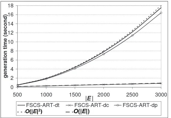
We experimentally evaluated the execution time of FSCS-ART-dc and
FSCS-ART-dp via some simulations. All simulations were conducted on a
machine with an Intel Pentium processor running at 3195 MHz and 1024
megabytes of RAM. The ART algorithms were implemented in C language
and compiled with GNU Compiler Collection (Version 3.3.4) (GCC, 2004).
FSCS-ART-dt, FSCS-ART-dc and FSCS-ART-dp were implemented in a 2D
space. For each algorithm, we recorded the time taken to select a number of
test cases, with |E| = 500,1000,1500,2000,2500 and 3000. The simulation
results are given in Figure 2, in which, x- and y-axes denote |E| and time
required to generate E, respectively. It is clearly shown that
FSCS-ART-dt and FSCS-ART-dp both require O(|E|2
) time to select |E| test cases,
while the execution time of FSCS-ART-dc is in O(|E|). In other words, the
experimental data are consistent with the above theoretical analysis.
4.2
Analysis of failure detection capabilities
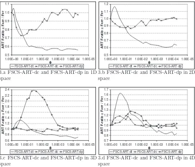
Some simulations (with settings identical to those given in Section 2.3) were
conducted to study the failure detection capabilities of FSCS-ART-dc and
FSCS-ART-dp. The size of candidate set k was set as 10, same as the
0 2 4 6 8 10 12 14 16 18
500 1000 1500 2000 2500 3000
|E|
g
e
n
e
ra
ti
o
n
t
im
e
(
s
e
c
o
n
d
)
FSCS-ART-dt FSCS-ART-dc FSCS-ART-dp
o o
Figure 2: Comparison of execution time among dt, FSCS-ART-dc and FSCS-ART-dp
Figure 3, which also includes the previous results of FSCS-ART-dt for ease
of comparison.
When simulations were conducted on FSCS-ART-dp, it was found that
it is often extremely difficult, if not impossible, for FSCS-ART-dp to detect
a failure, especially when dI is low (the explanation for such a phenomenon will be given later). Therefore, this study can only collect F-measures of
FSCS-ART-dp in 3D and 4D space. Figure 3 reports that FSCS-ART-dc
only marginally outperforms RT, and FSCS-ART-dp usually has a higher
F-measure than RT. In brief, neither discrepancy nor dispersion will result
in a good failure detection capability when each of them is applied as the
standalone test case selection criterion.
Intuitively speaking, an even spread of test cases implies a low
discrep-ancy and a low dispersion, but neither a low discrepdiscrep-ancy nor a low dispersion
necessarily implies an even spread of test cases. Therefore, it is
0.5 0.6 0.7 0.8 0.9 1.0 1.1 1.00E-05 1.00E-04 1.00E-03 1.00E-02 1.00E-01 1.00E+00 T ART F-ratio = F A R T / F R T
FSCS-ART-dt FSCS-ART-dc FSCS-ART-dp
3.a FSCS-ART-dc and FSCS-ART-dp in 1D space 0.5 0.6 0.7 0.8 0.9 1.0 1.1 1.2 1.00E-05 1.00E-04 1.00E-03 1.00E-02 1.00E-01 1.00E+00 T ART F-ratio = F A R T / F R T
FSCS-ART-dt FSCS-ART-dc FSCS-ART-dp
3.b FSCS-ART-dc and FSCS-ART-dp in 2D space 0.6 0.8 1.0 1.2 1.4 1.6 1.8 2.0 2.2 2.4 1.00E-05 1.00E-04 1.00E-03 1.00E-02 1.00E-01 1.00E+00 T ART F-ratio = F A R T / F R T
FSCS-ART-dt FSCS-ART-dc FSCS-ART-dp
3.c FSCS-ART-dc and FSCS-ART-dp in 3D space 0.7 0.8 0.9 1.0 1.1 1.2 1.3 1.4 1.5 1.6 1.7 1.00E-05 1.00E-04 1.00E-03 1.00E-02 1.00E-01 1.00E+00 T ART F-ratio = F A R T / F R T
FSCS-ART-dt FSCS-ART-dc FSCS-ART-dp
3.d FSCS-ART-dc and FSCS-ART-dp in 4D space
Figure 3: Failure detection capabilities of FSCS-ART-dc and FSCS-ART-dp
process may not deliver an even spread of test cases, and thus may not bring
a good failure detection capability.
4.3
Analysis of test case distributions
In order to further explain why these FSCS-ART-dc and FSCS-ART-dp
can-not perform better than RT, more simulations were conducted to investigate
their test case distributions (the experimental settings are identical to those
used in Section 2.4). The simulation results are reported in Figures 4 and 5,
in which, the previous results for FSCS-ART-dt and RT are also included for
0.00 0.10 0.20 0.30 0.40 0.50 0.60
0 2000 4000 6000 8000 10000
|E|
M
Disc
rep
an
cy
FSCS-ART-dt FSCS-ART-dc FSCS-ART-dp RT
4.a MDiscrepancy in 1D space
0.00 0.05 0.10 0.15 0.20 0.25 0.30 0.35 0.40 0.45
0 2000 4000 6000 8000 10000
|E|
M
Disc
rep
an
cy
FSCS-ART-dt FSCS-ART-dc FSCS-ART-dp RT
4.bMDiscrepancy in 2D space
0.00 0.05 0.10 0.15 0.20 0.25 0.30
0 2000 4000 6000 8000 10000
|E|
M
Disc
rep
an
cy
FSCS-ART-dt FSCS-ART-dc FSCS-ART-dp RT
4.c MDiscrepancy in 3D space
0.00 0.02 0.04 0.06 0.08 0.10 0.12 0.14 0.16 0.18 0.20
0 2000 4000 6000 8000 10000
|E|
M
Disc
rep
an
cy
FSCS-ART-dt FSCS-ART-dc FSCS-ART-dp RT
4.dMDiscrepancy in 4D space
Figure 4: MDiscrepancy of FSCS-ART-dc and FSCS-ART-dp
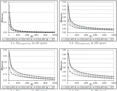
It is observed that FSCS-ART-dc always has a smaller MDiscrepancy than FSCS-ART-dt and RT, as intuitively expected; however, its MDispersion is larger than that of FSCS-ART-dt, and similar to that of RT. As observed
by Chen et al. (2007b), a good failure detection capability of an ART
al-gorithm is always associated with a small value of Mdispersion. FSCS-ART-dc does not have a smaller Mdispersion than RT, although it has a small
Mdiscrepancy. Therefore, it is understandable that FSCS-ART-dc does not sig-nificantly outperform RT. Given this observation, a small MDiscrepancy alone is not enough to imply a good failure detection capability of ART.
As far as FSCS-ART-dp is concerned, it can be found that FSCS-ART-dp
0.00 0.01 0.02 0.03
0 2000 4000 6000 8000 10000
|E|
M
Dispersion
FSCS-ART-dt FSCS-ART-dc FSCS-ART-dp RT
5.aMDispersion in 1D space
0.00 0.02 0.04 0.06 0.08 0.10 0.12 0.14 0.16
0 2000 4000 6000 8000 10000
|E|
M
Dispersion
FSCS-ART-dt FSCS-ART-dc FSCS-ART-dp RT
5.bMDispersion in 2D space
0.05 0.10 0.15 0.20 0.25 0.30
0 2000 4000 6000 8000 10000
|E|
M
Dispersion
FSCS-ART-dt FSCS-ART-dc FSCS-ART-dp RT
5.c MDispersion in 3D space
0.10 0.15 0.20 0.25 0.30 0.35 0.40 0.45
0 2000 4000 6000 8000 10000
|E|
M
Dispersion
FSCS-ART-dt FSCS-ART-dc FSCS-ART-dp RT
5.dMDispersion in 4D space
Figure 5: MDispersion of FSCS-ART-dc and FSCS-ART-dp
that of FSCS-ART-dt. The large value ofMDiscrepancy for FSCS-ART-dp may be due to the definition of dispersion used in this study. The intuition of
dis-persion is to measure the largest empty spherical region inside I. Given that
the sample points are uniformly distributed, the largest nearest neighbour
distance (Equation 4 in Section 2.4) is a good metric to reflect the size of
this empty spherical region. However, when FSCS-ART-dp solely uses such
a definition to select test cases without considering the uniform distribution,
it is quite likely that the selected test cases would be clustered into some
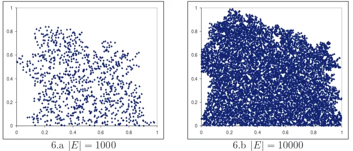
re-gions inside I. As an example to illustrate the cluster of test cases, Figure 6
shows test cases (denoted by diamond dots) selected by FSCS-ART-dp in a
test cases selected by FSCS-ART-dp are not evenly spread at all. This not
only explains why FSCS-ART-dp has a large MDiscrepancy, but also answers why FSCS-ART-dp has a poor failure detection capability. Briefly speaking,
a fairly large MDiscrepancy is always associated with a poor performance of an ART algorithm, no matter how small MDispersion is.
0 0.2 0.4 0.6 0.8 1
0 0.2 0.4 0.6 0.8 1
6.a |E|= 1000
0 0.2 0.4 0.6 0.8 1
0 0.2 0.4 0.6 0.8 1
6.b |E|= 10000
Figure 6: Some test cases selected by FSCS-ART-dp in 2D space
Another interesting phenomenon of FSCS-ART-dp is that its failure
de-tection capability andMDiscrepancy become better asdI increases. The reason behind such a phenomenon is explained as follows. Suppose that there are
two pointsp= (x1, x2,· · · , xdI) andq= (x1+∆x1, x2+∆x2,· · · , xdI+∆xdI),
wherexi andxi+ ∆xi denote the coordinates ofpand qon theith dimension
(i = 1,2,· · · , dI), respectively. Obviously, dist(p, q) =
q PdI
i=1(∆xi) 2. For
points p and q to be very close to each other, all |∆xi|s ought to be very small. Intuitively speaking, when dI is higher, it is less likely that all|∆xi|s have small values, and thus it is less likely for pand q to be physically
adja-cent. In other words, the uneven distribution of test cases in FSCS-ART-dp
5
Adaptive random testing based on
distri-bution metrics (DM-ART)
As discussed in Section 4, although discrepancy and dispersion measure
cer-tain aspects of the evenness of test case distribution, neither of them can
ensure an even spread of test cases if each of them is solely used as the test
case selection criterion in ART. Compared with these two criteria,Sdistance is a better test case selection criterion, because it gives FSCS-ART-dt a small
MDispersion, and also a good failure detection capability. However, as pointed out by Chen et al. (2007b),Sdistance is not perfect, because it may result in a relatively large MDiscrepancy and a poor performance for some special cases. In this section, we will investigate how to improve the performance of ART
by usingSdiscrepancy and Sdispersion as additional test case selection criteria to supplement Sdistance.
This study proposes some new algorithms, which use Sdiscrepancy and
Sdispersion to select test cases together with Sdistance. Since some of test case selection criteria in the new algorithms are originally from some distribution
metrics, the new algorithms are named asART based on distribution metrics (DM-ART).
5.1
DM-ART algorithms with two selection criteria
The algorithms proposed in this section, which include two levels of test
case selections, are called astwo-level DM-ART (2L-DM-ART). The detailed algorithm of 2L-DM-FSCS-ART is given in Figure 7.
In 2L-DM-FSCS-ART, two test case selection criteria, denoted by S1 and
S2, will be selected before the testing process (Statement 3 in Figure 7).
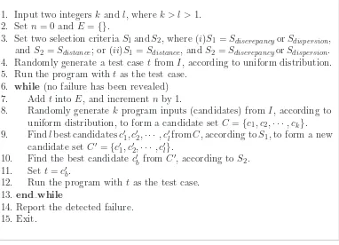
1. Input two integers k andl, wherek > l >1. 2. Set n= 0 and E={}.
3. Set two selection criteriaS1andS2, where (i)S1 =SdiscrepancyorSdispersion,
and S2 =Sdistance; or (ii)S1 =Sdistance, and S2 =SdiscrepancyorSdispersion.
4. Randomly generate a test case tfrom I, according to uniform distribution. 5. Run the program witht as the test case.
6. while(no failure has been revealed) 7. Addt intoE, and increment nby 1.
8. Randomly generate kprogram inputs (candidates) fromI, according to uniform distribution, to form a candidate set C={c1, c2,· · · , ck}.
9. Findlbest candidatesc′1, c′2,· · · , c′lfromC, according toS1, to form a new
candidate setC′ ={c′1, c′2,· · · , c′l}.
10. Find the best candidate c′b fromC′, according toS2.
11. Set t=c′b.
12. Run the program with tas the test case. 13.end while
14. Report the detected failure. 15. Exit.
Figure 7: The algorithm of 2L-DM-FSCS-ART
Sdispersion. Hence, there are totally four new ART algorithms. 2L-DM-FSCS-ART with S1 =Sdiscrepancy andS2 =Sdistance is referred to as
FSCS-ART-dc-dt. The other three algorithms are similarly referred to as FSCS-ART-dp-dt,
FSCS-ART-dt-dc, and FSCS-ART-dt-dp. Based on the results in Section 4.1,
we can conclude that the execution time of the 2L-DM-FSCS-ART algorithms
is in O(|E|2
).
It should be noted that it is not expected to have a good failure detection
capability when only Sdiscrepancy and Sdispersion are used together as the se-lection criteria. As shown in Section 4, both dc and
FSCS-ART-dp exhibit certain degrees of uneven distribution of test cases. However,
there does not exist any complementary relationship between discrepancy
will offset each other. Therefore, it is not intuitively expected that
FSCS-ART-dc-dp and FSCS-ART-dp-dc outperform RT. Our simulation results
on FSCS-ART-dc-dp and FSCS-ART-dp-dc are consistent with the above
intuitive expectation.
A series of simulations (with settings identical to those given in
Sec-tion 2.3) were conducted to investigate the failure detecSec-tion capabilities of
the 2L-DM-FSCS-ART algorithms given in Figure 7. In these simulations,
k is set as 10 to be consistent with previous studies of FSCS-ART-dt. l
in 2L-DM-FSCS-ART algorithms cannot be either too large (that is, close
to k) or too small (that is, close to 1); otherwise, one of the two selection
criteria will have an effectively dominating impact on the performance of
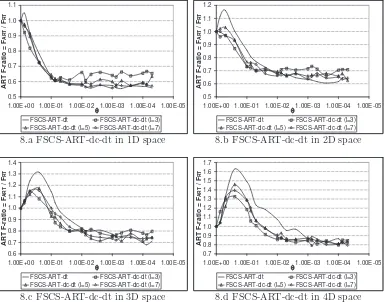
2L-DM-FSCS-ART. In these simulations, we set l = 3,5, or 7. Figures 8, 9, 10
and 11 report the simulation results on FSCS-ART-dc-dt,
FSCS-ART-dp-dt, FSCS-ART-dt-dc and FSCS-ART-dt-dp, respectively. It should be noted
that FSCS-ART-dp-dt with l = 3,5 and FSCS-ART-dt-dp with l = 5,7 in
1D space have the same problem as FSCS-ART-dp in lowdI cases, that is, an uneven distribution of test cases. Therefore, Figures 9 and 11 do not include
the data for these algorithms for 1D case. The reason why these algorithms
perform well for high dI cases have been given in Section 4.
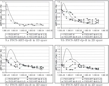
The following observations can be made from the simulation results.
• All 2L-DM-FSCS-ART algorithms outperform FSCS-ART-dt for the
cases of high θ and high dI.
• For 2L-DM-FSCS-ART algorithms withS2 =Sdistance (FSCS-ART-dc-dt and FSCS-ART-dp-(FSCS-ART-dc-dt), the failure detection capabilities improve
with the increase of l.
(FSCS-ART-dt-0.5 0.6 0.7 0.8 0.9 1.0 1.1 1.00E-05 1.00E-04 1.00E-03 1.00E-02 1.00E-01 1.00E+00 T A R T F -r a ti o = F A R T / F R T
FSCS-ART-dt FSCS-ART-dc-dt (l=3) FSCS-ART-dc-dt (l=5) FSCS-ART-dc-dt (l=7)
8.a FSCS-ART-dc-dt in 1D space
0.5 0.6 0.7 0.8 0.9 1.0 1.1 1.2 1.00E-05 1.00E-04 1.00E-03 1.00E-02 1.00E-01 1.00E+00 T A R T F -r a ti o = F A R T / F R T
FSCS-ART-dt FSCS-ART-dc-dt (l=3) FSCS-ART-dc-dt (l=5) FSCS-ART-dc-dt (l=7)
8.b FSCS-ART-dc-dt in 2D space
0.6 0.7 0.8 0.9 1.0 1.1 1.2 1.3 1.4 1.00E-05 1.00E-04 1.00E-03 1.00E-02 1.00E-01 1.00E+00 T A R T F -r a ti o = F A R T / F R T
FSCS-ART-dt FSCS-ART-dc-dt (l=3) FSCS-ART-dc-dt (l=5) FSCS-ART-dc-dt (l=7)
8.c FSCS-ART-dc-dt in 3D space
0.7 0.8 0.9 1.0 1.1 1.2 1.3 1.4 1.5 1.6 1.7 1.00E-05 1.00E-04 1.00E-03 1.00E-02 1.00E-01 1.00E+00 T A R T F -r a ti o = F A R T / F R T
FSCS-ART-dt FSCS-ART-dc-dt (l=3) FSCS-ART-dc-dt (l=5) FSCS-ART-dc-dt (l=7)
8.d FSCS-ART-dc-dt in 4D space
Figure 8: Failure detection capabilities of FSCS-ART-dc-dt
dc and FSCS-ART-dt-dp), the failure detection capabilities improve
with the decrease of l.
The first observation is consistent with the intuitive expectation. It has
been observed by (Chen et al., 2007b,c) that when θ and dI are high, the original FSCS-ART-dt algorithm does not perform well and does not evenly
distribute its test cases in terms of some distribution metrics. Since
2L-DM-FSCS-ART algorithms use these metrics to guide the test case selection
process, these algorithms are expected to have better failure detection
capa-bilities than the original FSCS-ART-dt under these situations. For the cases
0.5 0.6 0.7 0.8 0.9 1.0 1.1 1.00E-05 1.00E-04 1.00E-03 1.00E-02 1.00E-01 1.00E+00 T A R T F -r a ti o = F A R T / F R T
FSCS-ART-dt FSCS-ART-dp-dt (l=3) FSCS-ART-dp-dt (l=5) FSCS-ART-dp-dt (l=7)
9.a FSCS-ART-dp-dt in 1D space
0.5 0.6 0.7 0.8 0.9 1.0 1.1 1.2 1.00E-05 1.00E-04 1.00E-03 1.00E-02 1.00E-01 1.00E+00 T A R T F -r a ti o = F A R T / F R T
FSCS-ART-dt FSCS-ART-dp-dt (l=3) FSCS-ART-dp-dt (l=5) FSCS-ART-dp-dt (l=7)
9.b FSCS-ART-dp-dt in 2D space
0.6 0.7 0.8 0.9 1.0 1.1 1.2 1.3 1.4 1.00E-05 1.00E-04 1.00E-03 1.00E-02 1.00E-01 1.00E+00 T A R T F -r a ti o = F A R T / F R T
FSCS-ART-dt FSCS-ART-dp-dt (l=3) FSCS-ART-dp-dt (l=5) FSCS-ART-dp-dt (l=7)
9.c FSCS-ART-dp-dt in 3D space
0.7 0.8 0.9 1.0 1.1 1.2 1.3 1.4 1.5 1.6 1.7 1.00E-05 1.00E-04 1.00E-03 1.00E-02 1.00E-01 1.00E+00 T A R T F -r a ti o = F A R T / F R T
FSCS-ART-dt FSCS-ART-dp-dt (l=3) FSCS-ART-dp-dt (l=5) FSCS-ART-dp-dt (l=7)
9.d FSCS-ART-dp-dt in 4D space
Figure 9: Failure detection capabilities of FSCS-ART-dp-dt
becomes smaller, approaching to the theoretical bound which an optimal
test-ing method can reach without any information about failure locations (Chen
and Merkel, 2008). Therefore, it is understandable that 2L-DM-FSCS-ART
algorithms do not significantly decrease the FART whenθ is low or dI is low. The second and third observations are explained as follows. As mentioned
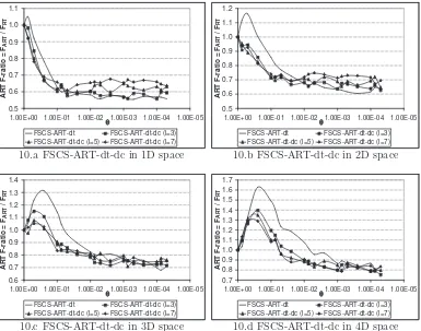
in Section 4, neither Sdiscrepancy nor Sdispersion is sufficient to ensure an even spread of test cases. These selection criteria must work together withSdistance. In FSCS-ART-dc-dt and FSCS-ART-dp-dt algorithms, the next test case
FSCS-ART-dt-0.5 0.6 0.7 0.8 0.9 1.0 1.1 1.00E-05 1.00E-04 1.00E-03 1.00E-02 1.00E-01 1.00E+00 T A R T F -r a ti o = F A R T / F R T
FSCS-ART-dt FSCS-ART-dt-dc (l=3) FSCS-ART-dt-dc (l=5) FSCS-ART-dt-dc (l=7)
10.a FSCS-ART-dt-dc in 1D space
0.5 0.6 0.7 0.8 0.9 1.0 1.1 1.2 1.00E-05 1.00E-04 1.00E-03 1.00E-02 1.00E-01 1.00E+00 T A R T F -r a ti o = F A R T / F R T
FSCS-ART-dt FSCS-ART-dt-dc (l=3) FSCS-ART-dt-dc (l=5) FSCS-ART-dt-dc (l=7)
10.b FSCS-ART-dt-dc in 2D space
0.6 0.7 0.8 0.9 1.0 1.1 1.2 1.3 1.4 1.00E-05 1.00E-04 1.00E-03 1.00E-02 1.00E-01 1.00E+00 T A R T F -r a ti o = F A R T / F R T
FSCS-ART-dt FSCS-ART-dt-dc (l=3) FSCS-ART-dt-dc (l=5) FSCS-ART-dt-dc (l=7)
10.c FSCS-ART-dt-dc in 3D space
0.7 0.8 0.9 1.0 1.1 1.2 1.3 1.4 1.5 1.6 1.7 1.00E-05 1.00E-04 1.00E-03 1.00E-02 1.00E-01 1.00E+00 T A R T F -r a ti o = F A R T / F R T
FSCS-ART-dt FSCS-ART-dt-dc (l=3) FSCS-ART-dt-dc (l=5) FSCS-ART-dt-dc (l=7)
10.d FSCS-ART-dt-dc in 4D space
Figure 10: Failure detection capabilities of FSCS-ART-dt-dc
dc and FSCS-ART-dt-dp algorithms,Sdistance is used to identifyl candidates amongst which Sdiscrepancy or Sdispersion is going to select one as a test case. Intuitively speaking, in these two algorithms, a smallerlimplies thatSdistance affects the ART performance more significantly thanSdiscrepancy orSdispersion.
5.2
DM-ART algorithms with three selection criteria
2L-DM-ART algorithms presented in the previous section can only adopt
one distribution metric as a test case selection criterion (the other
0.5 0.6 0.7 0.8 0.9 1.0 1.1 1.00E-05 1.00E-04 1.00E-03 1.00E-02 1.00E-01 1.00E+00 T A R T F -r a ti o = F A R T / F R T
FSCS-ART-dt FSCS-ART-dt-dp (l=3) FSCS-ART-dt-dp (l=5) FSCS-ART-dt-dp (l=7)
11.a FSCS-ART-dt-dp in 1D space
0.5 0.6 0.7 0.8 0.9 1.0 1.1 1.2 1.00E-05 1.00E-04 1.00E-03 1.00E-02 1.00E-01 1.00E+00 T A R T F -r a ti o = F A R T / F R T
FSCS-ART-dt FSCS-ART-dt-dp (l=3) FSCS-ART-dt-dp (l=5) FSCS-ART-dt-dp (l=7)
11.b FSCS-ART-dt-dp in 2D space
0.6 0.7 0.8 0.9 1.0 1.1 1.2 1.3 1.4 1.00E-05 1.00E-04 1.00E-03 1.00E-02 1.00E-01 1.00E+00 T A R T F -r a ti o = F A R T / F R T
FSCS-ART-dt FSCS-ART-dt-dp (l=3) FSCS-ART-dt-dp (l=5) FSCS-ART-dt-dp (l=7)
11.c FSCS-ART-dt-dp in 3D space
0.7 0.8 0.9 1.0 1.1 1.2 1.3 1.4 1.5 1.6 1.7 1.00E-05 1.00E-04 1.00E-03 1.00E-02 1.00E-01 1.00E+00 T A R T F -r a ti o = F A R T / F R T
FSCS-ART-dt FSCS-ART-dt-dp (l=3) FSCS-ART-dt-dp (l=5) FSCS-ART-dt-dp (l=7)
11.d FSCS-ART-dt-dp in 4D space
Figure 11: Failure detection capabilities of FSCS-ART-dt-dp
well asSdistance in the test case selection process. Figure 12 gives the detailed algorithm of 3L-DM-FSCS-ART.
As shown in Figure 12, 3L-DM-FSCS-ART will set three test case
selec-tion criteria prior to testing (Statement 3 in Figure 12), which are denoted
by Sa,Sb andSc, respectively. Six 3L-DM-FSCS-ART algorithms can be de-veloped, which can be referred to as FSCS-ART-dc-dp-dt (denoting 3L-DM-FSCS-ART with Sa =Sdiscrepancy, Sb =Sdispersion and Sc =Sdistance), FSCS-ART-dc-dt-dp, FSCS-ART-dp-dc-dt, FSCS-ART-dp-dt-dc,
FSCS-ART-dt-dc-dp, and FSCS-ART-dt-dp-dc. Like 2L-DM-FSCS-ART,
3L-DM-FSCS-ART algorithms also requireO(|E|2
) time to select |E| test cases.
1. Input three integers k,gand h, wherek > g > h >1. 2. Set n= 0 andE ={}.
3. Set three selection criteria Sa,Sb and Sc, whereSa,Sb,Sc = Sdiscrepancy,
Sdispersion, orSdistance, and Sa6=Sb 6=Sc.
4. Randomly generate a test case tfrom I, according to uniform distribution. 5. Run the program with tas the test case.
6. while (no failure has been revealed) 7. AddtintoE, and increment nby 1.
8. Randomly generatek program inputs (candidates) fromI, according to uniform distribution, to form a candidate set C={c1, c2,· · · , ck}.
9. Find g best candidates c′1, c′2,· · ·, c′g from C, according to Sa, to form a
new candidate set C′={c′1, c′2,· · · , c′g}.
10. Find h best candidatesc′′1, c′′2,· · · , c′′hfromC′, according to Sb, to form a
new candidate set C′′={c′′1, c′′2,· · · , c′′h}.
11. Find the best candidate c′′b fromC′, according toSc.
12. Sett=c′′b.
13. Run the program with tas the test case. 14. end while
15. Report the detected failure. 16. Exit.
Figure 12: The algorithm of 3L-DM-FSCS-ART
Section 2.3) to evaluate the failure detection capabilities of these
3L-DM-FSCS-ART algorithms. It was found that all 3L-DM-3L-DM-FSCS-ART algorithms
have more or less similar failure detection capabilities. We plot the ART
F-ratios of FSCS-ART-dc-dt-dp in Figure 13, which also includes the previous
simulation results of FSCS-ART-dt, FSCS-ART-dc-dt (l = 7),
FSCS-ART-dt-dp (l = 3) for ease of comparison. In our simulations, the values of g
andh for FSCS-ART-dc-dt-dp are set as 7 (similar to the optimal setting for
FSCS-ART-dc-dt shown in Section 5.1) and 3 (similar to the optimal setting
for FSCS-ART-dt-dp), respectively.
Based on Figure 13, we have the following observations.
0.5 0.6 0.7 0.8 0.9 1.0 1.1 1.00E-05 1.00E-04 1.00E-03 1.00E-02 1.00E-01 1.00E+00 T A R T F -r a ti o = F A R T / F R T FSCS-ART-dt FSCS-ART-dc-dt FSCS-ART-dt-dp FSCS-ART-dc-dt-dp
13.a Comparison in 1D space
0.5 0.6 0.7 0.8 0.9 1.0 1.1 1.2 1.00E-05 1.00E-04 1.00E-03 1.00E-02 1.00E-01 1.00E+00 T A R T F -r a ti o = F A R T / F R T FSCS-ART-dt FSCS-ART-dc-dt FSCS-ART-dt-dp FSCS-ART-dc-dt-dp
13.b Comparison in 2D space
0.6 0.7 0.8 0.9 1.0 1.1 1.2 1.3 1.4 1.00E-05 1.00E-04 1.00E-03 1.00E-02 1.00E-01 1.00E+00 T A R T F -r a ti o = F A R T / F R T FSCS-ART-dt FSCS-ART-dc-dt FSCS-ART-dt-dp FSCS-ART-dc-dt-dp
13.c Comparison in 3D space
0.7 0.8 0.9 1.0 1.1 1.2 1.3 1.4 1.5 1.6 1.7 1.00E-05 1.00E-04 1.00E-03 1.00E-02 1.00E-01 1.00E+00 T A R T F -r a ti o = F A R T / F R T FSCS-ART-dt FSCS-ART-dc-dt FSCS-ART-dt-dp FSCS-ART-dc-dt-dp
13.d Comparison in 4D space
Figure 13: Comparison of Failure detection capabilities for FSCS-ART-dt, FSCS-ART-dc-dt, FSCS-ART-dt-dp, FSCS-ART-dc-dt-dp
dI are high.
• For 1D and 2D cases, all three DM-ART algorithms have similar failure
detection capabilities.
• For 3D and 4D cases,
– When θ is very small (θ < 0.001), all three DM-ART algorithms
have similar performances.
– Whenθis very large (θ > 0.1), dt-dp and
FSCS-ART-dc-dt-dp have similar performances, which are better than that of
– Under other situations (0.001 < θ < 0.1), FSCS-ART-dc-dt and
FSCS-ART-dc-dt-dp have similar performances, which are better
than that of FSCS-ART-dt-dp.
As shown in Figure 13, among all three investigated DM-ART algorithms,
FSCS-ART-dc-dt-dp is the best enhancement to the original FSCS-ART-dt
algorithm for various dI and θ. This is consistent with the intuition that the more criteria are integrated in an ART algorithm, the better performance
the algorithm will have. Therefore, in the following sections, we only choose
FSCS-ART-dc-dt-dp as the target of our study.
5.3
Test case distributions of DM-ART
More simulations (with settings identical to those given in Section 2.4) were
conducted to collect the values of MDiscrepancy and MDispersion for FSCS-ART-dc-dt-dp. The simulations results are reported in Figures 14 and 15,
respectively. These figures also include the previous simulation results of
FSCS-ART-dt and RT for ease of comparison.
Based on the experimental data, we observe the followings.
• FSCS-ART-dc-dt-dp always has a smaller MDiscrepancy than FSCS-ART-dt.
• For 1D and 2D cases,MDispersion for FSCS-ART-dc-dt-dp is similar to that of FSCS-ART-dt.
• For 3D and 4D cases, FSCS-ART-dc-dt-dp has a marginally smaller
MDispersion than FSCS-ART-dt.
In brief, ART-dc-dt-dp spreads test cases more evenly than
0.00 0.02 0.04 0.06 0.08 0.10 0.12
0 2000 4000 |E|6000 8000 10000
M
Disc
rep
an
cy
FSCS-ART-dt FSCS-ART-dc-dt-dp RT
14.aMDiscrepancy in 1D space
0.00 0.02 0.04 0.06 0.08 0.10 0.12
0 2000 4000 |E|6000 8000 10000
M
Disc
rep
an
cy
FSCS-ART-dt FSCS-ART-dc-dt-dp RT
14.bMDiscrepancy in 2D space
0.00 0.01 0.02 0.03 0.04 0.05 0.06 0.07 0.08 0.09 0.10
0 2000 4000 |E|6000 8000 10000
M
Disc
rep
an
cy
FSCS-ART-dt FSCS-ART-dc-dt-dp RT
14.c MDiscrepancy in 3D space
0.00 0.01 0.02 0.03 0.04 0.05 0.06 0.07 0.08
0 2000 4000 |E|6000 8000 10000
M
Disc
rep
an
cy
FSCS-ART-dt FSCS-ART-dc-dt-dp RT
14.dMDiscrepancy in 4D space
Figure 14: MDiscrepancy of FSCS-ART-dc-dt-dp
ART that the more evenly test cases are spread, the better failure detection
capability an ART algorithm has.
5.4
Effectiveness of DM-ART on real-life programs
The original FSCS-ART-dt algorithm has been used to test some real-life
pro-grams (Chen et al., 2004). These propro-grams, which were published by ACM
(1980) and Press et al. (1986), were error-seeded using the technique of
muta-tion (Budd, 1981). For ease of comparison with the previous studies, we also
used these error-seeded programs to study the effectiveness of DM-ART. We
0.00 0.01 0.02 0.03
0 2000 4000 |E|6000 8000 10000
M
Dispersion
FSCS-ART-dt FSCS-ART-dc-dt-dp RT
15.aMDispersion in 1D space
0.00 0.02 0.04 0.06 0.08 0.10 0.12 0.14 0.16
0 2000 4000 |E|6000 8000 10000
M
Dispersion
FSCS-ART-dt FSCS-ART-dc-dt-dp RT
15.bMDispersion in 2D space
0.05 0.10 0.15 0.20 0.25 0.30
0 2000 4000 |E|6000 8000 10000
M
Dispersion
FSCS-ART-dt FSCS-ART-dc-dt-dp RT
15.c MDispersion in 3D space
0.10 0.15 0.20 0.25 0.30 0.35 0.40 0.45
0 2000 4000 |E|6000 8000 10000
M
Dispersion
FSCS-ART-dt FSCS-ART-dc-dt-dp RT
15.dMDispersion in 4D space
Figure 15: MDispersion of FSCS-ART-dc-dt-dp
The details of these 4 programs are given in Table 1.
In the simulations conducted in Sections 4.2, 5.1 and 5.2, various values
ofθ can be selected for study, and the predefined failure regions can reside in
any location inside I. However, θ and the location of failure regions in these
mutated programs cannot be varied easily to generate a sufficient number
of samples to achieve a statistically significant measurement of the failure
detection capability.
In this study, we aim to investigate the effectiveness of
FSCS-ART-dc-dt-dp under different scenarios (different θ and different locations of failure
regions). Therefore, we kept the same seeded errors, but randomly generated
Table 1: Program name, dimension, and seeded errors for each subject pro-gram
Program Dimension Number of seeded errors
AOR ROR SVR CR
airy 1 1
bessj 2 2 1 1
plgndr 3 1 2 2
el2 4 1 3 2 3
AOR arithmatic operator replacement
ROR relational operator replacement
SVR scalar variable replacement
CR constant replacement
Each randomly selected range value may yield a different θ and a different
location of the failure region within the input domain. The shape of the
failure region may also be affected. In this way, each subject program can
be tested under 100 distinct scenarios.
We used both FSCS-ART-dt and FSCS-ART-dc-dt-dp to test the subject
programs. The ART F-ratios of FSCS-ART-dt and FSCS-ART-dc-dt-dp on
these programs are reported by boxplots in Figure 16. Boxplots (Tukey,
1977), which are widely used in descriptive statistics, provide a convenient
way of depicting the distribution of a data set. In a box plot, the first
quartile (x.25), the median (x.50), and the third quartile (x.75) of a data set
are represented by the bottom edge, the central line, and the top edge of the
box, respectively. Upper and lower whiskers (denoted by small horizontal
lines outside the box) refer to the maximum and minimum values of a data
set, respectively. The whiskers and the box’s edges are connected by two
vertical lines. Boxplots in Figure 16 also include the mean values of ART
0.4 0.5 0.6 0.7 0.8 0.9 1.0
FSCS-ART-dt F-ratio FSCS-ART-dc-dt-dp F-ratio
16.a ART F-ratios onairy
0.5 0.6 0.7 0.8 0.9 1.0 1.1
FSCS-ART-dt F-ratio FSCS-ART-dc-dt-dp F-ratio
16.b ART F-ratios onbessj
0.4 0.5 0.6 0.7 0.8 0.9 1.0 1.1 1.2
FSCS-ART-dt F-ratio FSCS-ART-dc-dt-dp F-ratio
16.c ART F-ratios onplgndr
0.5 0.6 0.7 0.8 0.9 1.0 1.1 1.2
FSCS-ART-dt F-ratio FSCS-ART-dc-dt-dp F-ratio
16.d ART F-ratios onel2
Figure 16: Comparison of Effectiveness on real-life programs for FSCS-ART-dt and FSCS-ART-dc-FSCS-ART-dt-dp
Similar to what have been observed in the simulation studies reported
in Section 5.2, the failure detection capability of FSCS-ART-dc-dt-dp
de-pends on dI, but FSCS-ART-dc-dt-dp has a smaller mean value of ART F-ratios than FSCS-ART-dt. The use of boxplots in Figure 16 helps to show
that FSCS-ART-dc-dt-dp has a much smaller value range of ART F-ratios
than FSCS-ART-dt. Such an observation implies that FSCS-ART-dc-dt-dp
is more preferable to FSCS-ART-dt, not only because the former generally
has a better failure detection capability than the latter, but also because the
the location of failure region.
6
Discussion and Conclusion
Adaptive random testing (ART) was proposed to enhance the failure
detec-tion capability of random testing (RT) by evenly spreading test cases over the
input domain. In many ART algorithms, besides the random generation of
the program inputs, some test case selection criteria are additionally used to
ensure an even spread of random test cases. Though even spread is intuitively
simple, there does not exist a standard definition of even spread, needless to
say the existence of a standard measurement for the evenness of test case
dis-tribution. Research (Chen et al., 2007b) has been attempted to use various
distribution metrics to reflect, if not measure, how evenly an ART algorithm
spreads test cases. Previous studies have conclusively shown that some ART
algorithms, which are not regarded by certain distribution metrics as evenly
spreading their test cases, usually perform poorly. This correlation between
test case distribution and failure detection capability has motivated us to
develop some new ART algorithms, which apply these distribution metrics,
mainly discrepancy and dispersion, as test case selection criteria in ART.
We first studied some algorithms using each of these metrics as the
stan-dalone criterion to select test cases in ART. Our simulation results showed
that these ART algorithms have poor failure detection capabilities. This is
due to the fact that a low discrepancy and a low dispersion are just necessary
characteristics of an even spread of test cases, but not vice versa. In fact,
simply enforcing test cases to solely satisfy a single criterion leads to certain
degrees of uneven test case distribution.
of “far apart” in FSCS-ART (that is, keeping test cases as far apart from
one another as possible), and proposed a new family of ART algorithms,
namelyART based on distribution metrics (DM-ART). Two subcategories of DM-ART algorithms, namely 2L-DM-FSCS-ART and 3L-DM-FSCS-ART,
were investigated via simulations. The simulation results showed that by
keeping the “far apart” notion as the more influential test case selection
criterion, some DM-ART algorithms not only spread test cases more evenly,
but also have better failure detection capabilities than the original
FSCS-ART algorithm. It was also observed that one 3L-DM-FSCS-FSCS-ART algorithm,
namely FSCS-ART-dc-dt-dp, provides the best performance improvement
over the original FSCS-ART algorithm among all DM-ART algorithms. An
empirical study on FSCS-ART-dc-dt-dp further showed that as compared
with the original FSCS-ART algorithm, DM-ART has a failure detection
capability less dependent on the failure rate and the location of failure region.
In summary, the integration of discrepancy and dispersion with the notion
of “far apart” does improve both the evenness of the test case distribution
and the failure detection capability.
There are various definitions of discrepancy and dispersion in the
litera-ture, and we have only adopted the most commonly used definitions in this
study. It is interesting to further investigate the impacts of other definitions
of discrepancy and dispersion. Chen et al. (2007b) have pointed out that
the ART algorithms under their study may not well satisfy the definitions of
some distribution metrics. Restricted random testing, for example, generally
has a small dispersion, but a relatively large discrepancy, just like
FSCS-ART. Therefore, the innovative approach of this study, that is, adopting test
case distribution metrics as test case selection criteria in ART, can be equally
Acknowledgment
This research project is supported by an Australian Research Council
Dis-covery Grant (DP0880295).
References
ACM, 1980. Collected Algorithms from ACM. Association for Computing
Machinery.
Ammann, P. E., Knight, J. C., 1988. Data diversity: an approach to software
fault tolerance. IEEE Transactions on Computers 37 (4), 418–425.
Beizer, B., 1990. Software Testing Techniques. Van Nostrand Reinhold.
Bird, D. L., Munoz, C. U., 1983. Automatic generation of random
self-checking test cases. IBM Systems Journal 22 (3), 229–245.
Bishop, P. G., 1993. The variation of software survival times for different
operational input profiles. In: Proceedings of the 23rd International
Sym-posium on Fault-Tolerant Computing. pp. 98–107.
Branicky, M. S., LaValle, S. M., Olson, K., Yang, L., 2001. Quasi-randomized
path planning. In: Proceedings of the 2001 IEEE International Conference
on Robotics and Automation. IEEE Computer Society, pp. 1481–1487.
Budd, T. A., 1981. Mutation analysis: Ideas, examples, problems and
prospects. In: Chandrasekaran, B., Radicci, S. (Eds.), Computer Program
Chan, K. P., Chen, T. Y., Towey, D., 2006. Restricted random testing:
Adap-tive random testing by exclusion. International Journal of Software
Engi-neering and Knowledge EngiEngi-neering 16 (4), 553–584.
Chen, T. Y., Kuo, F.-C., Liu, H., 2007a. Distribution metric driven adaptive
random testing. In: Proceedings of the 7th International Conference on
Quality Software (QSIC 2007). pp. 274–279.
Chen, T. Y., Kuo, F.-C., Liu, H., 2007b. On test case distributions of adaptive
random testing. In: Proceedings of the 19th International Conference on
Software Engineering and Knowledge Engineering (SEKE 2007). pp. 141–
144.
Chen, T. Y., Kuo, F.-C., Zhou, Z. Q., 2007c. On favorable conditions for
adaptive random testing. International Journal of Software Engineering
and Knowledge Engineering 17 (6), 805–825.
Chen, T. Y., Leung, H., Mak, I. K., 2004. Adaptive random testing. In:
Proceedings of the 9th Asian Computing Science Conference. pp. 320–329.
Chen, T. Y., Merkel, R., 2007. Quasi-random testing. IEEE Transactions on
Reliability 56 (3), 562–568.
Chen, T. Y., Merkel, R., 2008. An upper bound on software testing
effective-ness. ACM Transactions on Software Engineering and Methodology 17 (3),
16:1–16:27.
Ciupa, I., Leitner, A., Oriol, M., Meyer, B., 2006. Object distance and
its application to adaptive random testing of object-oriented programs.
In: Proceedings of the First International Workshop on Random Testing
Ciupa, I., Leitner, A., Oriol, M., Meyer, B., 2008. ARTOO: adaptive random
testing for object-oriented software. In: Proceedings of the 30th
Interna-tional Conference on Software Engineering (ICSE’08). ACM Press, pp.
71–80.
Dab´oczi, T., Koll´ar, I., Simon, G., Megyeri, T., 2003. Automatic testing of
graphical user interfaces. In: Proceedings of the 20th IEEE
Instrumenta-tion and Measurement Technology Conference 2003 (IMTC ’03). Vail, CO,
USA, pp. 441–445.
Finelli, G. B., 1991. NASA software failure characterization experiments.
Reliability Engineering and System Safety 32 (1–2), 155–169.
Forrester, J. E., Miller, B. P., 2000. An empirical study of the robustness of
Windows NT applications using random testing. In: Proceedings of the
4th USENIX Windows Systems Symposium. Seattle, pp. 59–68.
GCC, 2004. GNU compiler collection, http://gcc.gnu.org.
Girard, E., Rault, J., 1973. A programming technique for software reliability.
In: Proceedings of 1973 IEEE Symposium on Computer Software
Relia-bility. IEEE, pp. 44–50.
Godefroid, P., Klarlund, N., Sen, K., 2005. DART: directed automated
ran-dom testing. In: Proceedings of ACM SIGPLAN Conference on
Program-ming Language Design and Implementation (PLDI 2005). ACM Press, pp.
213–223.
Hailpern, B., Santhanam, P., 2002. Software debugging, testing, and
Hamlet, R., 2002. Random testing. In: Marciniak, J. (Ed.), Encyclopedia of
Software Engineering, 2nd Edition. John Wiley & Sons.
Hua, L. K., Wang, Y., 1981. Applications of Number Theory to Numerical
Analysis. Springer, Berlin.
Kuo, F.-C., 2006. On adaptive random testing. Ph.D. thesis, Faculty of
Infor-mation and Communications Technologies, Swinburne University of
Tech-nology.
Mayer, J., 2005. Lattice-based adaptive random testing. In: Proceedings of
the 20th IEEE/ACM International Conference on Automated Software
Engineering (ASE 2005). ACM, New York, USA, pp. 333–336.
Mayer, J., Guderlie, R., 2006. On random testing of image processing
ap-plications. In: Proceedings of the 6th International Conference on Quality
Software (QSIC 2006). IEEE Computer Society, pp. 85–92.
Mayer, J., Schneckenburger, C., 2006. An empirical analysis and comparison
of random testing techniques. In: Proceedings of the 2006 ACM/IEEE
In-ternational Symposium on Empirical Software Engineering (ISESE 2006).
ACM Press, pp. 105–114.
Merkel, R., 2004. Enhancement of adaptive random testing. Ph.D. thesis,
School of Information Technology, Swinburne University of Technology.
Miller, B. P., Fredriksen, L., So, B., 1990. An empirical study of the reliability
of UNIX utilities. Communications of the ACM 33 (12), 32–44.
Miller, B. P., Koski, D., Lee, C. P., Maganty, V., Murthy, R., Natarajan,
UNIX utilities and services. Tech. Rep. CS-TR-1995-1268, University of
Wisconsin.
Myers, G. J., 2004. The Art of Software Testing, 2nd Edition. John Wiley
and Sons, revised and updated by T. Badgett and T. M. Thomas with C.
Sandler.
Niederreiter, H., 1986. Quasi-monte carlo methods for global optimization.
In: Proceedings of the 4th Pannonian Symposium on Mathematical
Statis-tics. pp. 251–267.
Niederreiter, H., 1992. Random Number Generation and Quasi-Monte-Carlo
Methods. SIAM.
NIST, 2002. The economic impacts of inadequate infrastructure for software
testing, http://www.nist.gov/director/prog-ofc/report02-3.pdf,
National Institute of Standards and Technology, Gaithersburg, Maryland,
USA.
Press, W. H., Flannery, B. P., Teukolsky, S. A., Vetterling, W. T., 1986.
Numerical Recipes. Cambridge Unversity Press.
Regehr, J., 2005. Random testing of interrupt-driven software. In:
Proceed-ings of the 5th ACM International Conference on Embedded Software
(EM-SOFT’05). ACM Press, pp. 290–298.
Slutz, D., 1998. Massive stochastic testing of SQL. In: Proceedings of the
24th International Conference on Very Large Databases (VLDB 1998). pp.
618–622.
Thayer, R. A., Lipow, M., Nelson, E. C., 1978. Software Reliability.
Tukey, J. W., 1977. Exploratory Data Analysis. Addison-Wesley.
West, C. H., Tosi, A., 1995. Experiences with a random test driver. Computer
Networks and ISDN Systems 27, 1163–1174.
White, L. J., Cohen, E. I., 1980. A domain strategy for computer program
testing. IEEE Transactions on Software Engineering 6 (3), 247–257.
Yoshikawa, T., Shimura, K., Ozawa, T., 2003. Random program generator
for Java JIT compiler test system. In: Proceedings of the 3rd International