Path, theme and narrative in open plan exhibition settings

(1)

29.1

29

Keywords

museum exhibition, spatial layout, path, theme, narrative, learning

[email protected] [email protected] [email protected]

NickDalton <[email protected]>

Path, theme and narrative in open plan exhibition settings

John Peponis1_{, Ruth Conroy Dalton}1_{, Jean Wineman}2_{, Nick SheepDalton}3

1_{Georgia Institute of Technology} 2_{University of Michigan}

3 _{Georgia Regional Transportation Authority}

Abstract

Three arguments are made based on the analysis of science exhibitions. First, sufficiently refined techniques of spatial analysis allow us to model the impact of layout upon visitors’ paths, even in moderately sized open plans which allow almost random patterns of movement and relatively unobstructed visibility. Second, newly developed or adapted techniques of analysis allow us to make a transition from modeling the mechanics of spatial movement (the way in which movement is affected by the distribution of obstacles and boundaries), to modeling the manner in which movement might register additional aspects of visual information. Third, the advantages of such purely spatial modes of analysis extend into providing us with a sharper understanding of some of the pragmatic constrains within which exhibition content is conceived and designed.

Introducing the question: how do permissive open layouts influence patterns of exhibition exploration?

This paper presents new research on the relationship between visitor behavior and layout in science exhibition settings1_{. The aims are largely methodological and}

(2)

29.2

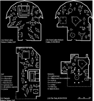
The analysis deals with two traveling science exhibitions, each in two different settings (Figure 1). Both were created by the same organization, the Carnegie Science Center. “ZAP surgery” presented new technologies for medical operations. “Robotics”, introduced the principles that govern robotic design and function. The first was studied at The Great Lakes Science Center, Cleveland, and at the Carnegie Science Center, Pittsburgh. The second was studied at The Tech museum in San Jose and at the Great Lakes Science Center, Cleveland. All studies were completed in academic year 2000-2001. In both instances, almost all individual exhibits were interactive, with the exception of a small number that consisted in video presentations or in visual information only. Also, individual exhibits were designed to provide a self contained amount of information, but also classified according to conceptual themes. For example, in the ZAP exhibition displays were visually and spatially coordinated according to the following themes: gamma rays, laser beams, cryosurgery, endoscopy and ultra sound. In the case of Robotics, the presentation of displays referred to aspects of acting, sensing, areas of application, demonstration of use, and exhibits aimed at “junior” visitors. The conceptual themes were made more evident visually in the ZAP exhibition, based on the use of color both on individual exhibits and on the background to the corresponding zones of the exhibition. In the case of Robotics, conceptual themes were less strongly suggested, either by spatial zoning, or through visual design. In both instances, however, the classification of individual exhibits by a smaller set of themes was objectively documented in the literature accompanying the exhibitions, whether in printed catalogues, or in the corresponding web-pages.

The exhibition settings under study were simple open plans as shown in Figure 1. Many individual exhibits, or small groups of individual exhibits were free standing, whether suggesting a peripheral approach, from all sides, or a directional approach, with a clear distinction between front, back and lateral views. Other exhibits are located against the perimeter boundary, or against structural elements. The temporary

(3)

29.3

exhibition area itself varied from the relatively compact and clearly bounded shape of the Great Lakes Science Center, to the more elongated shape of the Carnegie Center, or the more compact but weakly bounded space at The Tech. The few large individual exhibits, such as the ZAP Cam Simulation Capsule in the ZAP exhibition, or the Basketball Robot Arm in the Robotics exhibition, tend to be so located against the area boundary as to divide space while at the same time acting as focal points of visual attention. There is ample cross visibility between individual exhibits. The arrangement allows a plethora of alternative exploration paths, as there are relatively few impediments to movement. In short, the arrangements under study are not overly didactic, either in the sense of imposing a deliberate sequence to the pattern of exploration, or in the sense of framing successive visual fields to control visual groupings and cross comparisons.

From the point of view of layout, the exhibition settings under study imply a mode of discourse where units of knowledge (the units corresponding to individual exhibit elements) are relatively self-contained and where the overall message arises from the quasi-random accumulation of such units. The visitor is left with the task of re-constructing the exhibition narrative; understanding the layout itself appears to be no challenge. As used here, the term “narrative” refers to the manner in which the contents of individual exhibits can be conceptually related. For example some displays suggest that robot design involves the combination of many simple joints such that complex movements can result from the combination of simpler motions; other displays suggest that movements of the hand can be translated into mechanical movements through simple devices; a third group of displays suggests that information of some sort must be coded and translated in such a way as to cause various motions; a fourth group suggests that sensors can be used to receive information about changes in the environment. Putting such ideas together, the visitor can think of robots as mechanisms capable of not only transferring movement but also of receiving coded instructions for movement, or of processing environmental information in order to produce such instructions. The word “narrative”, therefore, refers to the arrangement of information in logical sequence in a manner that yields more complex insights. In many exhibitions, the sequence in which information is to be received is largely dictated by the layout. In the exhibitions under study, this was not the case.

(4)

29.4

visual content, an engagement was registered. Contacts include engagements but not all contacts involve engagement. Repeat contacts and repeat engagements were also registered. Each individual exhibit was thus assigned its corresponding “1st Contact”, “1st Engagement”, “Repeat Contact” and “Repeat Engagement” counts. Repeat counts include the 1st occurrence of the relevant behavior. In the rest of this paper, these counts will be the behavioral performance scores assigned to individual exhibits. Table 1 provides a basic quantitative profile of visitor behavior. Visitors spent between 16 and 23 minutes per exhibition, depending on the setting. Each individual exhibit was contacted by between 46 and 59% and engaged by between 13% and 24% of the total number of visitors, also depending on the setting.

ZAP ZAP

Surgery Surgery Robotics Robotics G.t Lakes Carnegie G.t Lakes San Jose Science Science Science Tech Center Center Center Museum

Number of visitors tracked 96 97 103 102

Avg. Total Time (minutes) 22.7 15.9 21.1 16.6

Avg. Total Stop Time (minutes) 18.8 12.5 17.4 12.8

Avg. # of Contacts 28.26 23.80 32.10 23.11

Avg. # 1st Contacts per Individual exhibit 48.74 44.44 57.71 60.60 %Visitors Contacting each Individual exhibit 51% 46% 56% 59% Avg. # Repeat Contacts per Individual exhibit 92.52 80.78 100.68 98.04

Avg. # of Engagements 10.38 6.03 12.51 9.82

Avg. # 1st Engagements per Individual exhibit 19.93 13.00 24.74 24.40 %Visitors Engaging each Individual exhibit 21% 13% 24% .24%

Avg. # Repeat Engagements per Individual exhibit 31.78 17.63 38.55 36.88

Individual visitors were described according to the sequence of contacts, including engagements, and the sequence of engagements only. These sequences were transcribed into strings of characters from the original graphic records taken in the museum settings. For example, a string describing a visitor’s path as a sequence of contacts is {3,2,1,4,8,12,13,36,37,35,23,1,3,2,19} where each number stands for an individual exhibit; the string describing the same visitors’ engagements is {3,36,3}; the first string transcribed according to themes becomes {CCCULLLSKGGCCCE} (exhibits 3,2,1 belong to the same theme C, exhibit 4 belongs to theme U and so on), while the second becomes {CSC}. The strings according to individual exhibit and the strings according to themes were the basis for computing the appropriate behavioral attraction scores for each individual exhibit, either based on contacts or on engagements only. Individual visitors are also characterized by the total time they spent in the exhibition.

The simple positional model: the statistical effects of spatial arrangement upon otherwise unconstrained search paths and engagement patterns.

At the simplest level, the spatial structure of layouts arises as objects and boundaries are placed in space. Objects and boundaries work as obstructions that limit potential movement. The greater the limitations upon movement, the more movement patterns

(5)

29.5

are distributed according to the layout. Accordingly, the first model developed here is called “positional” in that spatial structure is considered only according to the effects of positioning objects and boundaries in space. No attempt is made to recognize the additional effects of the specific semantic content of individual exhibits. Nor do we deal with the ways in which individual exhibits may be related across space by such characteristics as common coloring, background lighting and so on. However, the fact that each exhibit has a primary face and an associated contact region in its immediate spatial neighborhood, where visitors must stand in order to engage it, is acknowledged. The spatial positioning of individual exhibits is described according to the properties of the corresponding contact regions. In other words, the position of exhibits is described according to the properties of the occupiable space immediately in front of them.

(6)

29.6

MD(i) is the Mean Depth from vantage point i

d(i-j) is the number of intervening polygons between vantage points i and j k is the number of vantage points in the system

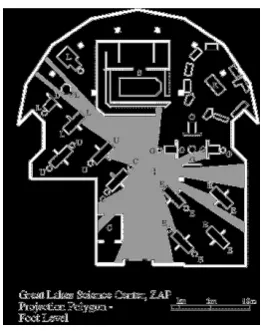
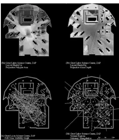
“Area” and “Mean Depth” values were computed using “Omnivista”, software written by Nick Dalton and Ruth Conroy-Dalton, both members of the research team. Omnivista was used to flood-fill all navigable space within each of the exhibition sites with a grid of vantage points, and to generate visibility polygons from these locations. Various properties are then computed for each visibility polygon, including area; perimeter; compactness; minimum, mean and maximum radial length; and drift, or the vector distance between the vantage point and the center of gravity of the polygon. “Area” and “Mean Depth” proved to have greater relevance to our research. Average Area and Mean Depth Values were computed for each individual exhibit contact region, taking all the vantage points encompassed by the region into account. The grid used to flood-fill space is 30cm by 30cm and so each Contact region encompassed several, or even many grid units. Figure 3a shows a layout shaded according to the area of projection polygons drawn from each square of the 30cm by 30 cm grid. Likewise, Figure 3b shows the same layout shaded according to the mean depth of the polygons.

The cross visibility between individual exhibits was described by directed graphs, whose nodes represent individual exhibit contact regions, and whose arcs describe the visibility of one position from another. These graphs were established empirically, in the field. The use of directed graphs was dictated by the fact that when two exhibits are positioned in front of each other and face in the same direction, the front side of the exhibit at the back is not visible to a person engaging the exhibit at the front, while the later is visible to a person engaging the exhibit at the back.

Figure 2: Example of a projection polygon

⊇

MD

( )i

=

d i

( )

−

j

j=1

(7)

29.7

One directed graph describes relations of Full Visibility while another records relations of Partial Visibility. “Full Visibility” was defined as being able to see another individual exhibit so as to determine its nature and contents. “Partial Visibility” was defined as being able to see enough information to determine the presence of another individual exhibit, but not its contents or its nature. Thus, the “Full Visibility” graph is a subset of the “Partial Visibility” graph. Cross Visibility graphs were analyzed using Pajek, software for graph analysis developed by V Baragelj and A Mrvar at the Department for Theoretical Computer Science and the Faculty of Social Sciences at the University of Ljubljana, Slovenia (http://vlado.fmf.uni-lj.si/pub/networks/ pajek). Of the various measures computed by Pajek, the most useful for our research was the simplest, namely degree. The degree of a node measures the number of arcs incident upon it. As we deal with directed graphs, a distinction is drawn between degree “in to” and degree “out from” a node. In order to be consistent with the terminology of previous studies, we will use the term “Connectivity” rather than degree. We will show that “Connectivity in to” a node is a good predictor of behaviors. It is important that our measure of connectivity is not confused with similar measures as applied to non-directed graphs. Figure 3c shows the full cross visibility directed graph overlaid upon a sample layout.

Table 2 presents a simple quantitative profile of the four settings. It shows that each individual exhibit can be directly reached from at least 8% and from up to 14% of the total exhibition area, depending on the setting. Also, no more than 3 direction changes are ever necessary to go from any point within an exhibition to another. Regarding cross-visibility, the table shows that between 1/3 and 2/3 of all

Figure 3: Visual representations of the main spatial descriptors for one of the settings

⊇

MD

( )i

=

d i

( )

−

j

j=1

(8)

29.8

other individual exhibits are at least partially visible from each individual exhibit. These numbers confirm the permissive and open character of these layouts regarding the potential exploration paths taken by visitors.

ZAP ZAP

Total Exhibition Area (square meters) 724 707 724 498 # of Individual exhibits(excludes children’s area) 27 27 35 25 Average full individual exhibit cross- visibility 21.8% 12.5% 19.4% 36.6% from other individual exhibits (% of all individual exhibits)

Average partial individual exhibit cross-visibility 41.8% 28.9% 51.7% 59.9% from other individual exhibits (% of all individual exhibits)

Avg. Projection Polygon Area (Square meters) 83.24 54.81 102.93 58.72 (from which an individual exhibit can be reached directly)

Avg. Projection Polygon Area as proportion of total Area 11.5% 7.8% 14.2% 11.8% Avg. Projection Polygon Mean Depth (direction 2.472 2.280 1.958 2.067 changes needed to reach from one position to another)

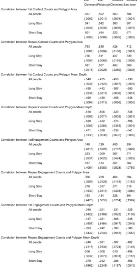
Table 3 presents linear correlation coefficients between the Area and Mean Depth of projection polygons corresponding to individual exhibits and four measures of behavioral attraction presented above, namely “1St Contact”, “Repeat Contacts”, “1st Engagement”, “Repeat Engagements”. The decision to look for linear correlations was based on a previous visual inspection of the scatter plots. Correlations are provided for three samples, all people observed, that is about hundred people per setting, the 25% of the people that spent more time in the exhibitions, and the 25% of the people that stayed less time. Thus, the table presents 96 correlations in total.

Contact counts are significantly and powerfully correlated with polygon Area, with 22 out of 24 correlations significant at the 1% level and stronger than 0.5, the other 2 correlations being also significant but only at the 5% level. Correlations with Mean Depth are less consistent. Only 15 out of 24 correlations are significant at the 1% level and another 7 at the 5% level. The average correlation for Area is 0.588 while for Mean Depth -0.507 (a negative correlation indicating that greater depth is associated with less contacts). Engagement counts are not consistently correlated with polygon properties. Only 2 out of 24 correlations with Area is significant at the 1% level and another 2 at the 5% level, a total of only 4 out of 24 correlations. Only one correlation with Mean Depth out of 24 is significant at the 1% level with another 2 significant at the 5% level. However, all significant correlations pertain to the Robotics exhibition. This will be discussed later. Here, we draw the conclusion that the most elementary consequence of the spatial arrangement of individual exhibits, namely the variation of direct accessibility, has a powerful effect on the manner in which the exhibitions are explored, as indexed by the distribution of contacts. Interestingly, layout seems to work similarly for people that stay longer and people that stay shorter lengths of time, without indication that longer lengths of stay are associated with any pattern of spatial learning that would register in terms of a stronger

(9)

29.9

association between spatial properties and navigation choices. Active engagement, however, is much less affected by spatial properties. We might infer that layout structures the search pattern, in an almost mechanical way, based on its most simple local properties. By contrast, engaging the individual exhibits would appear to be a function of decisions independent of layout, decisions which may perhaps arise based on the perceptual or cognitive appeal of exhibits. Further analysis, however, suggests that even the degree to which individual exhibits are engaged is affected by spatial parameters, as will be shown next.

ZAP ZAP Robotics Robotics ClevelandPittsburghClevelandSan Jose Correlation between 1st Contact Counts and Polygon Area

All people .657 .592 .563 .704

(.0002) (.0011) (.0004) (.0001)

Long Stay .541 .542 .583 .601

(.0036) (.0035) (.0006) (.0015)

Short Stay .601 .494 .522 .671

(.0009) (.0088) (.0026) (.0002) Correlation between Repeat Contact Counts and Polygon Area

All people .753 .635 .426 .712

(.0001) (.0004) (.0108) (.0001)

Long Stay .736 .511 .427 .639

(.0001) (.0065) (.0165) (.0006)

Short Stay .581 .557 .402 .669

(.0015) (.0025) (.0250) (.0003) Correlation between 1st Contact Counts and Polygon Mean Depth

All people -.540 -.475 -.458 -.736

(.0037) (.0123) (.0057) (.0001)

Long Stay -.435 -.442 -.507 -.690

(.0234) (.0211) (.0036) (.0001)

Short Stay -.490 -.480 -.458 -.648

(.0094) (.0113) (.0096) (.0005) Correlation between Repeat Contact Counts and Polygon Mean Depth

All people -.618 -.506 -.329 -.735

(.0006) (.0071) (.0539) (.0001)

Long Stay -.620 -.422 -.374 -.706

(.0006) (.0284) (.0383) (.0001)

Short Stay -.471 -.538 -.338 -.641

(.0130) (.0038) (.0632) (.0005) Correlation between 1stEngagement Counts and Polygon Area

All people .148 .129 .405 .354

(.4615) (.5226) (.0157) (.0829)

Long Stay .223 -.009 .367 .571

(.2631) (.9625) (.0424) (.0029)

Short Stay .167 .134 .351 .362

(.4051) (.5053) (.0528) (.0750) Correlation between Repeat Engagement Counts and Polygon Area

All people .366 .228 .404 .504

(.0605) (.2528) (.0161) (.0183)

Long Stay .276 -.037 .371 .518

(.1630) (.9317) (.0398) (.0080)

Short Stay .153 .134 .328 .304

(.4473) (.5053) (.0714) (.1399) Correlation between 1st Engagement Counts and Polygon Mean Depth

All people -.040 -.021 -.331 -.325

(.8422) (.9168) (.0525) (.1130)

Long Stay -.137 -.021 -.308 -.545

(.4957) (.9164) (.0917) (.0048)

Short Stay -.093 -.242 -.306 -.388

(.6432) (.2249) (.0943) (.0552) Correlation between Repeat Engagement Counts and Polygon Mean Depth

All people -.248 -.061 -.307 -.482

(.2117) (.7634) (.0724) (.0148)

Long Stay -206 -.008 -310 -.498

(.3037) (.9677) (.0901) (.0112)

Short Stay -.079 -.242 -.286 -.356

(.6962) (.2249) (.1187) (.0810)

Table 3: Correlations between meas-ures of the properties of projection polygons and measures of individual exhibit attraction

(10)

29.10

Table 4 presents linear correlations between the Full and Partial measures of individual exhibit cross visibility (Connectivity in to) and the same four measures of behavioral attraction. The decision to look for linear correlations was based upon a prior visual inspection of the scatter plots. The format and number of correlations shown is the same as in Table 1. Full cross visibility is not consistently correlated with contacts with 11 out of 24 correlations (including correlations for the whole population, as well as the 25% upper and lower percentiles of the population sorted by length of stay) significant at the 1% level and 4 at the 5% level. However, all of the strong and significant correlations (at 1%) occur in the Great Lakes Science

ZAP ZAP Robotics Robotics

Cleveland Pittsburgh Cleveland San Jose Correlation between 1st Contact Counts and Full Cross Visibility

All people 0.664 0.273 0.694 0.312

-0.0001 -0.1676 -0.0001 -0.1287

Long Stay 0.591 0.432 0.727 0.433

-0.0007 -0.0245 -0.0001 -0.0305

Short Stay 0.537 0.268 0.536 0.062

-0.0027 -0.176 -0.0019 -0.7702

Correlation between Repeat Contact Counts and Full Cross Visibility

All people 0.632 0.201 0.624 0.329

-0.0002 -0.3145 -0.0002 -0.1083

Long Stay 0.601 0.276 0.714 0.476

-0.0006 -0.1637 -0.0001 -0.0161

Short Stay 0.488 0.233 0.448 0.02

-0.0073 -0.2432 -0.0114 -0.9257

Correlation between 1st Contact Counts and Partial Cross Visibility

All people 0.699 0.246 0.791 0.595

-0.0001 -0.2153 -0.0001 (.00170

Long Stay 0.595 0.417 0.818 0.681

-0.0007 -0.0304 -0.0001 -0.0002

Short Stay 0.565 0.266 0.704 0.315

-0.0014 -0.1795 -0.0001 -0.125

Correlation between Repeat Contact Counts and Partial Cross Visibility

All people 0.682 0.203 0.718 0.596

-0.0001 -0.3109 -0.0001 -0.0017

Long Stay 0.59 0.328 0.731 0.655

-0.0008 -0.0951 -0.0001 -0.0004

Short Stay 0.53 0.259 0.636 0.286

-0.0031 -0.1917 -0.0001 (.16610

Correlation between 1st Engagement Counts Full Cross Visibility

All people 0.489 0.407 0.573 0.035

-0.0071 -0.0354 -0.0007 -0.8677

Long Stay 0.461 0.538 0.64 0.27

-0.0118 -0.0038 -0.0001 -0.192

Short Stay 0.508 0.407 0.455 0.141

-0.0049 -0.0349 -0.0101 -0.5013

Correlation between Repeat Engagement Counts and Full Cross Visibility

All people 0.652 0.38 0.633 0.15

-0.0001 -0.0504 -0.0001 -0.474

Long Stay 0.499 0.614 0.672 0.279

-0.0059 -0.0007 -0.0001 -0.1765

Short Stay 0.494 0.407 0.424 0.156

-0.0064 -0.0349 -0.0175 -0.4552

Correlation between 1st Engagement Counts and Partial Cross Visibility

All people 0.474 0.3 0.665 0.413

-0.0093 -0.1281 -0.0001 -0.04

Long Stay 0.436 0.463 0.659 0.617

-0.0181 -0.015 -0.0001 -0.001

Short Stay 0.543 0.422 0.623 0.318

-0.0023 -0.0284 -0.0002 -0.0887

Correlation between Repeat Engagement Counts and Partial Cross Visibility

All people 0.668 0.236 0.707 0.57

-0.0001 -0.2358 -0.0001 -0.003

Long Stay 0.473 0.497 0.676 0.604

-0.0096 -0.0083 -0.0001 -0.0014

Short Stay 0.533 0.422 0.601 0.353

-0.0029 -0.0284 -0.0004 -0.0832

(11)

29.11

Center, not only for the ZAP but also for the Robotics exhibition. There is no way that this bias can be reliably interpreted on a small sample of cases. However, we observe that the temporary exhibition area involved has a compact shape and a clearly delimited boundary, so as to both encourage cross visibility and filter out extraneous visual information. Partial cross visibility is more consistently correlated with contact counts 16 out of 24 correlations significant at the 1% level and another at the 5% level. Once again, the correlations are mostly associated with the Great Lakes Science Center.

Cross visibility has quite powerful effects upon the pattern of engagement. Full cross visibility is correlated with engagement counts with 11 out of 24 correlations significant at the 1% level and another 6 at the 5% level. Only in the case of Robotics at The Tech are no correlations significant. Partial cross visibility is even more consistently related with engagement counts with 15 correlations significant at the 1% level and another 4 at the 5% level. We draw the conclusion that exhibit cross visibility affects the pattern of engagement far more than the more generic properties of layouts such as direct accessibility or mean depth. Exhibits that become visible from other exhibits stand higher chances of attracting more active engagement. Furthermore, we can perhaps detect an informal pattern of conscious spatial responses. If we look at the comparison between correlations obtained for the people that stayed longer and those that stayed shorter amounts of time, in 10 out of 16 cases (there are 16 pairs of correlations to be compared) the behavior of the people staying longer is more strongly associated with cross visibility while the pair of correlations compared are both significant at least at the 5% level. One additional case follows the same pattern but the correlation for people that stayed less time is not significant. In 2 cases none of the relevant correlations is significant, while in 2 other cases the behavior of the people that stayed a shorted length of time is more strongly correlated with cross-visibility than the behavior of the people that stayed longer. We concluded that there is good evidence that as people stay longer, the visibility of individual exhibits from other individual exhibits has a more detectible effect upon decisions to engage individual exhibits.

(12)

29.12

Cleveland Pittsburgh Cleveland San Jose

ZAP ZAP Robotics Robotics

All Engagements string length 10 4 12 9

All Engagements Early Area ((sq m) 65.82 58.72 101.66 67.31 All Engagements Late Area ((sq m) 70.69 62.37 118.23 61.84

All Engagements Early Mean Depth 2.39 2.18 1.956 2.03

All Engagements Late Mean Depth 2.26 2.30 1.882 2.03

All Engagements Early Full Visibility 5.4 6 8 10.75

All Engagements Late Full Visibility 11.4 11 8.83 12.5

All Engagements Early Partial Visibility 13.4 9 21.83 19.25 All Engagements Late Partial Visibility 18.8 17.5 22.17 20.5

Shortest Engagements string length 3 1 9 6

Shortest Engagements Early Area (sq m) 30.82 NA 102.23 89.08 Shortest Engagements Late Area (sq m) 30.82 NA 125.98 62.17

Shortest Engagements Early Mean Depth 2.52 NA 1.98 1.93

Shortest Engagements Late Mean Depth 2.52 NA 1.889 2.01

Shortest Engagements Early Full Visibility 9 N/A 8.5 10.33

Shortest Engagements Late Full Visibility 9 N/A 7 11

Shortest Engagements Early Partial Visibility 18 N/A 23.75 16.67 Shortest Engagements Late Partial Visibility 18 N/A 18 22.33

Longest Engagements string length 15 11 19 14

Longest Engagements Early Area (sq m) 75.35 54.14 107.43 70.01 Longest Engagements Late Area (sq m) 62.96 45.08 105,26 60.53

Longest Engagements Early Mean Depth 2.28 2.42 1.972 1.99

Longest Engagements Late Mean Depth 2.34 2.63 1.908 2.08

Longest Engagements Early Full Visibility 8.71 7.8 9 9.86

Longest Engagements Late Full Visibility 5.14 3.2 20.67 12.43 Longest Engagements Early Partial Visibility 14.43 14.8 8.44 18.43 Longest Engagements Late Partial Visibility 11.71 7.4 20.78 19.14

All contacts string length 22 20 24 24

All Contacts Early Area (sq m) 115.01 72.76 112.9 69.8

All Contacts Late Area (sq m) 120.67 57.59 121.9 63.35

All Contacts Early Mean Depth 2.15 2.29 1.91 1.96

All Contacts Late Mean Depth 2.13 2.41 1.90 2.02

All Contacts Early Full Visibility 10.27 5.2 8 11.17

All Contacts Late Full Visibility 10.09 4.6 9.08 10.33

All Contacts Early partial Visibility 15.64 9.5 20.17 18.67 All Contacts Late Partial Visibility 16.64 10.6 22.25 18.5

Shortest Contacts string length 13 10 19 15

Shortest Contacts Early Area (sq m) 134.58 70.2 123.21 69.14 Shortest Contacts Late Area (sq m) 132.14 73.15 122.98 70.02

Shortest Contacts Early Mean Depth 2.10 2.30 1.87 2.00

Shortest Contacts Late Mean Depth 2.92 2.30 1.87 1.97

Shortest Contacts Early Full Visibility 11.5 6.6 8.56 13.29 Shortest Contacts Late Partial Visibility 9.67 4.2 8.56 8.14 Shortest Contacts Early partial Visibility 18 11 21.56 18.71 Shortest Contacts Late Partial Visibility 16.67 8.8 20.67 18.71

Longest Contacts string length 36 35 40 29

Longest Contacts Early Area (sq m) 87.39 57.22 119.18 67.85 Longest Contacts Late Area (sq m) 124.92 47.11 113.85 64.3

Longest Contacts Early Mean Depth 2.27 2.44 1.89 1.97

Longest Contacts Late Mean Depth 2.11 2.61 1.91 1.99

Longest Contacts Early Full Visibility 8.11 3.76 9.35 12 Longest Contacts Late Partial Visibility 13 3.88 7.6 11.27 Longest Contacts Early partial Visibility 14.67 8.82 21.25 19.57 Longest Contacts Late Partial Visibility 18 8.82 21 18.67

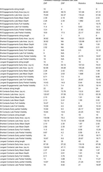
Table 5: Comparative data for the early and later halves of strings representative of all visitors’ paths, the shortest 25% of visi-tors’ paths and the longest 25% visitors paths

(13)

29.13

the fewest transformations to be changed to represent each of the other route strings in the sample. Figure 4 shows the most representative contacts and engagements strings for one of the settings. In addition to the most representative contact and engagement strings for each setting, we also determined the most representative strings of the corresponding 50% of the sample that included the longest paths, and the 50% of the sample that included the shortest paths. Thus, six strings were derived for each setting. We checked whether the average Area and the average Mean Depth of the projection polygons corresponding to each node was significantly different for the first and second halves of the strings. We found no such tendency. Indeed, strings appeared to oscillate between more and less accessible positions throughout their length. Thus, the pattern of accessibility has no strong effect upon the sequencing of exploration and individual exhibit engagement, even though, as we have shown above, it affects the frequency of contacts.

(14)

Path, theme and narrative in open plan exhibition settings

29.14

The compositional model: the statistical effects of labeling and the cognitiveorientation of search paths and engagement patterns.

The modified conceptual model to be developed next, arises from analyzing visitors’ paths as strings by theme. The question we ask is this: do exhibits carrying the same thematic label appear sequentially within the overall string representing a path, or are they dispersed? We call the corresponding property “categorization”. A string is strongly categorized if individual exhibits belonging to the same theme occur in uninterrupted sequences and weakly categorized if individual exhibits belonging to one label are interspaced with individual exhibits belonging to other labels. Categorization arises as exhibits are positioned to take into account of each other and to potentially function as collective and distributed destinations, in ways that do not directly obstruct movement. Hence we call the model to be developed here compositional, to distinguish it from the positional model in which exhibits are treated as individual obstructions and destinations.

First, we characterized strings as a whole according to whether they were strongly or weakly categorized. The aggregate categorization factor of a string measures the extent to which individual exhibits that bear the same label are visited in succession rather than at dispersed intervals along the path taken by an individual visitor. The exhibitions were designed in such a way that each exhibit belonged to a single theme and therefore carried a single thematic label. Higher aggregate categorization factors indicate that the visitor tended to visit individual exhibits bearing the same label as a group, before moving to individual exhibits bearing another label. Aggregate categorization factors are relativized to take into account the number of individual exhibits visited per label as well as the total length of the path (indexed by the number of individual exhibits it encompasses). The formula for the ACF of a string is:

ACF is the Aggregate Categorization Factor k is the number of themes represented in the string L is the length of the string

T is the number of transitions in the string regardless of theme

A is the number of transitions between string nodes belonging to different themes

N is the number of members of the theme with the greatest number of members within the string

Examples: For string “EEEEUUCUEE”, k=3, L=10, T=9, A=4, N= 6, L-N=4, N-1=5, Amax= 9-12+10+1=8, Amin=3-1=2, ACF=(8-4)/(8-2)=0.667 For string “EUEU”, k=2, L=4, T=3, A=3, N=2, L-N=2, N-1=1, Amax=3, Amin=1, ACF=(3-3)/(3-1)=0 For string “EEE”, A=0, ACF=1

Second, we categorized each label taken separately as being strongly or weakly categorized within the strings representing visitors’ paths within an exhibition setting. Given the description of visitors’ paths as strings by themes, we defined the categorization index per label per string as follows:

CL(lg) is the Categorization Index of label “l” in string “g” A(lg) is the number of members of label “l” in the string S(lg) is the number of segments in which label “l” occurs

E(lg) is the number of members of label “l” that occur either first or last in the string, and can assume values 0, or 1, or 2. In the special case that the string is composed of a single occurrence of label “l”, the value is 2.

Examples: For string “EEEUCU” evaluated for label “C”, A(lC)=1, S(lC)=1, E(lC)=0, 2S(lC -E(lC =2, CL(lC)= (1-1+1)/(2-0)=0.5 For the same string evaluated for label “E”, A(lE)=3, S(lE)=1, E(lE)=1, 2S(lE)-E(lE)=1, C(lE)=(3-1+1)/(2-1)=3 For the same string evaluated for label “U” A(lU)=2, S(lU)=2, E(lU)=1, 2S(lU)- E(lU)=4-1=3, CL(lU)=(2-2+1)/(4-1)=1/3=0.333 For string EEE, evaluated for label “E”, A(lE)=3, S(lE)=1, E(lE)=2, 2S(lE)-E(lE)=2-2=0, CL(lE)=3

The formula essentially provides as with a ratio of string transitions that are internal to a label “l”, that is transitions which connect two successive individual exhibits belonging to that label, over transitions that are external to a label “l”, that is transitions which connect an individual exhibit belonging to a label to an individual exhibit not belonging to the same label. The overall Categorization Index for a label, CI(lg) is defined as the average of CI(lg) for all strings “g” in which the label “l” occurs. The analysis of individual strings by labels was done on Excel worksheets.

Plans needed to be similarly analyzed to determine how far individual exhibits bearing the same thematic label, were spatially adjacent so as to encourage sequential viewing, or dispersed. We called the property whereby individual exhibits bearing the same thematic label are spatially adjacent “grouping”. In strongly grouped layouts, individual exhibits belonging to the same label are packed in close adjacency. In weakly grouped layouts, individual exhibits belonging to the same label are dispersed in different parts of the overall exhibition. A grouping index was developed as follows. First, a Voronoi diagram and Delaunay triangulation was obtained for each layout, after treating each individual exhibit as a point corresponding to its contact region. Delaunay Triangulation was conducted using XYZ GeoBench version 5.05 (free downloadable software), copyright 1999, P. Schorn, Department of Computer Science, Swiss Federal Institute of Technology, Zurich. An example is provided in figure 3d. The aim of this exercise was to provide us with a consistent way for determining the set of neighbors of each individual exhibit, even though the individual exhibits are irregularly distributed over the layout. Given a set of anchor points

)

Amin =

−

E

( )lg

)

=

0,CL

(16)

29.16

distributed over an area (here the individual exhibit interface positions) the Voronoi diagram divides space such that each region comprises all other points which are closest from a given anchor. Thus, the Voronoi diagram provides a convenient convention for assigning to each individual exhibit a convex polygon territory, such that no part of the layout remains unassigned. We do not claim that the Voronoi polygons represent the “attraction area” corresponding to an individual exhibit in any otherwise compelling manner: it is possible that some exhibits are visible and able to attract from well outside the area assigned to them in the Voronoi diagram, as it is also possible that from some positions in that area the specific contents of the exhibits cannot easily be read. The neighbors of an exhibit are unambiguously defined as the set of other exhibits whose Voronoi regions share a boundary with its region. Determining these neighbors if facilitated by considering the Delaunay triangulation, a graph where nodes represent points (here individual exhibit interfaces) and arcs represent shared boundaries of corresponding Voronoi regions.

The plans were analyzed to determine the number of Delaunay arcs corresponding to adjacencies between individual exhibits belonging to the same thematic label and the number of Delaunay arcs corresponding to adjacencies between individual exhibits belonging to different thematic labels. Here, the adjacencies under consideration also represent permeable connections, since we are dealing with open plan layouts. Two grouping indexes were obtained based on the foregoing representations. The individual exhibit-sensitive grouping index, GE(l) for easy reference, is the average of the ratio “internal”/”external” Delaunay arcs, computed for each set of individual exhibits corresponding to the same label “l”. The label-sensitive grouping index, GL(l) for easy reference, is the ratio “sum of internal”/ ”sum of external” Delaunay arcs considering all the individual exhibits belonging to the same label. Thus, GE(l) is an average of ratios, while GL(l) is a ratio of sums.

(17)

29.17

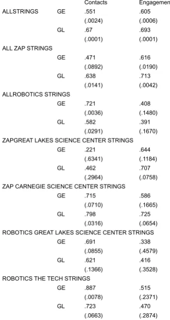
were analyzed not only by setting but also at different levels of aggregation, in order to allow for statistical significance in the results. When all settings are considered as a single set, there is a strong and significant correlation between the thematic categorization of paths and the spatial grouping of layouts. The correlations are even stronger for engagements than for contacts. This merits some comment. Contacts are to some extent sequenced according to the constraints imposed by layout: it is not possible to avoid the spaces which mediate between any origin and destination of a given transition from one individual exhibit of interest to another. Thus, it might even be hypothesized that had visitors moved randomly, their contacts would appear thematically categorized in direct proportion to the extent that the plans were thematically grouped. Such a hypothesis could not apply to engagements with similar plausibility. Engagements reflect a conscious decision which is not dictated by the pattern of adjacencies of the layout. The categorization of engagements would, therefore, indicate more clearly a cognitive registration of thematic labels, as compared to the categorization of contacts. The fact that when data are aggregated the spatial grouping of themes affects more powerfully the categorization of engagements than the categorization of contacts suggests that behaviors reflect the cognitive registration of thematic labels.

When we look at the analysis by setting, correlations between path categorization and layout grouping are stronger for the ZAP exhibition settings than they are for the Robotics settings. In fact, in the Robotics settings the correlation between categorization and grouping is only significant with respect to contacts, not with respect to engagements. This is consistent with the fact that in the case of the ZAP exhibition, thematic labels were not only more clearly grouped spatially, but also more clearly expressed visually, through the use of color, not only on the individual exhibits themselves, but also, through projections, in the background surfaces. However, only 1 of the 16 correlations computed for individual setting is significant at 1% and only an additional one at 5%. The lack of statistical significance, despite strong correlations, arises from the small number of thematic labels.

The second model developed here suggests that the process of relatively unstructured and locally driven exploration implied by the first model can be more globally and probabilistically constrained by making the thematic organization of exhibits more evident. This has two kinds of implications. First, it suggests that designers who develop the means to distinguish individual exhibits and also to group them spatially according to thematic label, can influence the pattern of visitor exploration. This is of special interest since thematic differentiation can be pursued without imposition of strict exploration sequences. Second, individual exhibit design, and the corresponding layout of knowledge units over an entire exhibition, could

ZAP! ZAP!

Surgery Surgery Robotics Robotics G.t Lakes Carnegie G.t Lakes San Jose Science Science Science Tech Center Center Center Museum

Number of visitors tracked 96 97 103 102 Avg. Total Time (minutes) 22.7 15.9 21.1 16.6 Avg. Total Stop Time (minutes) 18.8 12.5 17.4 12.8 Avg. # of Contacts 28.26 23.80 32.10 23.11 Avg. # 1st Contacts per Individual exhibit 48.74 44.44 57.71 60.60 %Visitors Contacting each Individual exhibit 51% 46% 56% 59% Avg. # Repeat Contacts per Individual exhibit 92.52 80.78 100.68 98.04 Avg. # of Engagements 10.38 6.03 12.51 9.82 Avg. # 1st Engagements per Individual exhibit 19.93 13.00 24.74 24.40 %Visitors Engaging each Individual exhibit 21% 13% 24% .24% Avg. # Repeat Engagements per Individual exhibit 31.78 17.63 38.55 36.88

Contacts Engagements ALLSTRINGS

GE .551 .605 (.0024) (.0006) GL .67 .693

(.0001) (.0001) ALL ZAP STRINGS

GE .471 .616 (.0892) (.0190) GL .638 .713

(.0141) (.0042) ALLROBOTICS STRINGS

GE .721 .408 (.0036) (.1480) GL .582 .391

(.0291) (.1670) ZAPGREAT LAKES SCIENCE CENTER STRINGS

GE .221 .644 (.6341) (.1184) GL .462 .707

(.2964) (.0758) ZAP CARNEGIE SCIENCE CENTER STRINGS

GE .715 .586 (.0710) (.1665) GL .798 .725

(.0316) (.0654) ROBOTICS GREAT LAKES SCIENCE CENTER STRINGS GE .691 .338

(.0855) (.4579) GL .621 .416

(.1366) (.3528) ROBOTICS THE TECH STRINGS

GE .887 .515 (.0078) (.2371) GL .723 .470

(18)

29.18

proceed on the assumption that search patterns can either be allowed to repeatedly intersect thematic groupings, or be channeled more systematically according to those groupings. By implication, thematically linked individual exhibits could be treated as contributing to a more constrained and structured pattern of accumulation of information.

Table 6: Aggregate String Categorization and Spatial Grouping Factors for the four Settings

Contacts Engagements

ALLSTRINGS GE .551 .605

(.0024) (.0006)

GL .67 .693

(.0001) (.0001) ALL ZAP STRINGS

GE .471 .616

(.0892) (.0190)

GL .638 .713

(.0141) (.0042) ALLROBOTICS STRINGS

GE .721 .408

(.0036) (.1480)

GL .582 .391

(.0291) (.1670) ZAPGREAT LAKES SCIENCE CENTER STRINGS

GE .221 .644

(.6341) (.1184)

GL .462 .707

(.2964) (.0758) ZAP CARNEGIE SCIENCE CENTER STRINGS

GE .715 .586

(.0710) (.1665)

GL .798 .725

(.0316) (.0654) ROBOTICS GREAT LAKES SCIENCE CENTER STRINGS

GE .691 .338

(.0855) (.4579)

GL .621 .416

(.1366) (.3528) ROBOTICS THE TECH STRINGS

GE .887 .515

(.0078) (.2371)

GL .723 .470

(.0663) (.2874)

Table 7: Correlations between the grouping of themes in the layout and the categorization of path strings representing interfaces and stops

(significance shown in parentheses)

ZAP ZAP

Contacts: Average Aggregate Categorization Factor 0.546 0.61 0.428 0.355 Engagements: Average Aggregate Categorization Factor 0.781 0.771 0.553 0.525 Spatial Grouping of Exhibition Theme 60.06% 59.70% 37.35% 48.06% (Individual exhibit Sensitive Index)

(19)

29.19

Discussion

Two general methodological and one general theoretical argument can arise from the foregoing arguments. The first methodological argument concerns the description of spatial behaviors. Once visitors’ paths are transcribed as strings of various characters, whether representing individual exhibits or themes, the development of various techniques for analyzing the structure of strings is critical to our ability to enrich the systematic description of spatial behaviors. One innovation of the research reported here is that strings were analyzed not only so that behavioral scores could be assigned to particular spatial positions (the individual exhibit interfaces), but also so that the spatial structure implicit in the string could itself be treated as descriptive data in its own right. The second methodological argument concerns the description of layouts themselves. On the one hand, this description can be refined through the development of more sensitive analytical techniques, such as the analysis of a plan according to the projection polygons that can be generated from a fine reference grid overlaid upon it. Software such as Omnivista makes such analysis relatively easy and such software is increasingly available. On the other hand, however, techniques must also be developed in order to capture how conceptual structures become embedded in layout design, including conceptual structures that are expressed through visual form. For example, a set of individual exhibits can be grouped not only by virtue of compact adjacency coupled to label homogeneity, but also by virtue of being nested inside a spatial region defined through the visual treatment of the surrounding perimeter, or the elaboration of the ceiling, or indeed lighting, none of which need to literally disrupt movement. Our discussion of the manner in which themes are spatially defined is an elementary step in the direction of developing richer descriptions of exhibition arrangements. There would appear to be much more room for innovation. Future work must not only draw further distinctions between descriptions of the spatial arrangement of individual exhibits which take into account various forms of labeling from descriptions which do not, but also continuously test whether descriptions sensitive to labeling can be linked to functional implications that can be inferred from observable spatial dimensions of behavior.

(20)

29.20

our perception of how objects might be related. From an analytical point of view, cognitive compositioning can initially be conceptualized as the addition of relationships between objects which are otherwise equivalent with respect to their positioning within a pattern of obstructions to visibility or access. Whether these relationships arise from common thematic labels associated with consistent coloring, or through the elaboration of lighting, or through decorative means of various sorts (all of which are present in the ZAP exhibition in varying degrees) is immaterial to this definition.

Notes

The research reported in the article was funded by a National Science Foundation Informal Science Education Grant, #9911829, with Dr. Jean Wineman as Principal Investigator and Dr. John Peponis as co Principal Investigator.

References

Benedikt, M. L., 1979, “To Take Hold of Space: Isovists and Isovist Fields”, Environment and Planning (B), 6, 47-65

Choi, Y. K., 1999, "The morphology of exploration and encounter in museum layouts", Environment and Planning (B): Planning and Design,26, pp. 241-250

Conroy-Dalton, 2001, “The secret is to follow your nose”, in J. Peponis, J. Wineman and S. Bafna (eds.),

Proceedings of the 3rd International Symposium on Space Syntax, Ann Arbor, A. Alfred Taubman College of Architecture and Urban Planning

Levenstein, V. I., 1965, “Binary Codes Capable of Correcting Deletions, Insertions and Reversals”, Diklady Akademii Nauk SSR (Russian), 163 (4), pp. 845-8

Turner, A., Doxa, M., O’Sullivan, D., Penn, A., 2001, “From isovists to visibility graphs: a methodology for the analysis of architectural space”, Environment and Planning B: Planning and Design, 28,