Adaptive Least Square Approximation For Fitting Scattered Data

(1)

ISSN 2348 – 7968

Adaptive Least Square Approximation for fitting scattered data

Alvin ASIMIP

1

P

1

P

Department of Mathematics Engineering, Polytechnic University of Tirana, Tirana, Albania

Abstract

This paper consists in the comparison of two adaptive least square approximation algorithms for fitting scattered data. The first part will present the Knot Insertion and Knot Removal algorithms. The second part consists in three experiments. For the experiments we consider the Franke’s test functions. All the fits are evaluated on a grid of 40 x 40 equally spaced points in the unit square. We will use Matlab for the evaluation of each approximation fit with Gaussian basic function with a shape parameter

ε

=

5.5

. The data sites used in this paper can be downloaded at 23TUhttp://www.math.unipd.it/~demarchi/TAA2010/U23T.

Keywords: 25TMeshfree Methods, Least Square Approximation,

Knot Insertion, Knot Removal, Numerical Methods, Matlab.

1. Introduction

Suppose we are given a set of data and we want to deduce conclusions from the process we are studying. This set of data consists in measurements and locations at which these measurements were obtained. Our goal is to find the rule in which this process develops. Thus, we are trying to find a function

Ρ

_f which is a “good” fit to the data, in order to gather information at locations different from those at which we obtained our measurements. If we want

Ρ

_f to exactly match the given measurements at the corresponding locations, this process is called Interpolation. If the locations of the given data do not lie on a regular grid, then the process is called scattered data interpolation.

Many times it makes more sense that

Ρ

_f does not match exactly the given measurements at the corresponding locations, for example if the data are contaminated with noise, or if we have a big amount of data. In these cases an approximation fit seems to be much more appropriate. This strategy consist in choosing M-data sites as centers for the basis functions, from N-data sites (N>M).

2. Adaptive Last Square Approximation

2.1 Knot Insertion Algorithm

In order to improve the quality of a given approximation based on a linear combination of basis functions, a classical used technique is to adaptively increase the number of basis functions used for the fit. This can be achieved by adding new knots to the existing ones. This approach was explored at [1] for multiquadrics on

R

2 and for radial basis functions (RBF) on spheres in [2].

Problem: We are given an amount of N data points, and we want to fit them with a RBF approximant within a given tolerance. We first fit the data with a RBF approximant based on few initial knots, and then find the “worst” data location with the largest error. In this location a new knot is inserted. This procedure continues as long as the last squares error exceeds a given tolerance.

Algorithm 1:

1. Let data sites

χ =

{ ,...,

x

₁

x

_N

}

, data

f

_i, and a tolerance tol be given.

2. Choose M initial knots

Ξ =

{ ,...,

ξ

₁

ξ

_M

}

. 3. Calculate the least square fit

1

( )

( ,

)

M

f j j

j

Q x

c

φ ξ

x

=

∑

4. Calculate the error

2 1

[

( )]

N

i f i i

e

f

Q x

=

∑

−

While e > tol do

5. “Weight” each data point

x

₁

,...,

x

_N, according to its error component

|

( ) |,

1,...,

.

i i f i

w

=

f

−

Q

x

i

=

N

(2)

{ },

x

_v

M

1. Ξ = Ξ ∪

=

+

7. Recalculate fit and associated error

The approximant is evaluated when the given tolerance is reached. For each iteration of this algorithm we have to solve one linear last square problem. The associated matrix A of these systems has full rank, since initial knots and the other knots inserted in each iteration are data sites. Another important thing of the algorithm is that no multiple knots are created (which leads to a rank deficiency).

Finally, a maximum iterations stop criteria is necessary if it is not possible to reach the given tolerance.

2.2 Knot Removal Algorithm

The idea of Knot Removal was motivated by the need of data reduction, but it can be used for adaptive approximation [3].

Problem: We are given an amount of N data points, and we want to fit them with a RBF approximant within a given tolerance. We first start with a god fit ( e,g an interpolation to the data) and then reduce the number of knots used until a given tolerance is reached. The follow algorithm was suggested in [2] for adaptive least squares approximation on spheres.

Algorithm 2:

1. Let data sites

χ =

{ ,...,

x

₁

x

_N

}

, data

f

_i, and a tolerance tol be given.

2. Choose M initial knots

Ξ =

{ ,...,

ξ

₁

ξ

_M

}

. 3. Calculate the least square fit

1

( )

( ,

)

M

f j j

j

Q x

c

φ ξ

x

=

∑

4. Calculate the error

2 1

[

( )]

N

i f i i

e

f

Q x

=

∑

−

While e < tol do

5. “Weight” each knot

ξ

₁

,...,

ξ

M, according to its

least square error, i.e form *

\ { },

ξ

_j

Ξ = Ξ

and calculate wights:

* 2

1

[

( )] ,

f

N

j i i

i

w

f

Q x

=

∑

−

where * *

( )

( ,

)

N j j

Q

x

=

∑

c

φ ξ

x

is the approximation based on

Ξ = Ξ

*

\ { },

ξ

_j 6. Find the knot

ξ

_µ with lowest weight

w

_µ and

permanently remove it *

\ { },

ξ

_µ

M

1. Ξ = Ξ

=

−

7. Recalculate fit and associated error.

The approximant is evaluated after the given tolerance is reached. Even in this algorithm a linear system is solved in each iteration in order to solve M least squares problems. If the initial knots are chosen at the data site, there will be no problems with the collocation matrix becoming rank deficient.

3. Numerical experiments and results

For the experiments we consider the Franke’s test functions (1) 2 2 2 2 2 2 2 2 1 1 1

(9 1) (9 1) [(9 2) (9 2) ]

49 10

4

1

[(9 7) (9 3) ] ₍₉ ₄₎ ₍₉ ₇₎ 4

3

3 ( , )

4

1

1 (1)

2

5

x y x y

x y _x _y

f x y

e

− + − + − − + − − − + − ₋ ₋ ₋ ₋

=

+

−

All the fits are evaluated on a grid of 40 x 40 equally spaced points in the unit square. We will use Matlab for the evaluation of each approximation fit with Gaussian basic function with a shape parameter

ε

=

5.5

(2).

2 2

2

|| || ₂

( )

e x xk

,

(2)

k

x

e

x

− −

Φ

=

∈



For each case we will compute the maximum error and the RMS error according to (3)

_

||

(3)

40

f f

Max err

Q

f

Q

f

RMS

∞ ∞

=

−

=

where

Q

_f

−

evaluated approximant on evaluation points

f

−

exact solution (Franke’s function )

40 – number of evaluation points

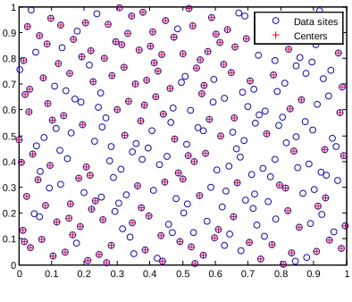
First experiment:

(3)

display the data sites and figure 2 display the Gaussian evaluated fit.

Fig.1 289 data sites and 154 knots

We start the Knot insertion “algorithm 1” with one random data site as a knot in the unit square, and then end up with 154 knots to reach the wanted tolerance tol=1e-004.

Fig.2 Least squares approximation using Knot Insertion Algorithm to Franke’s function

Second experiment:

As in the first experiment, we use 289 Halton data site and Gaussian basic function with a shape parameter

ε

=

5.5

but now use Knot Removal algorithm 2 with tol=0.5 with an interpolant to all 289 data values. Figure 3 display the data sites and figure 4 display the Gaussian evaluated fit

Fig .3 289 data sites and 153 knots.

In this case, we started with 289 data sites. The knot removal algorithm begins with an interpolant to all 289 data values. Tolerance tol=0.5 was reached with 153 knots.

Fig.4 Least squares approximation using Knot Removal Algorithm to Franke’s function

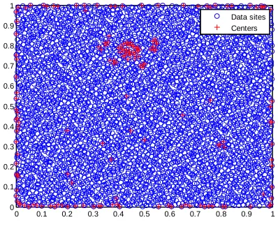
Third experiment:

As a final experiment we consider N=4225 Haltoin points and Gaussian basic function with a shape parameter

5.5 ε

=

and then use Knot Insertion algorithm 1 with tol=1e-0.004 starting with 1 data site as center for the basis functions. Figure 5 display the data sites and figure 6 display the Gaussian evaluated fit.

0 0.1 0.2 0.3 0.4 0.5 0.6 0.7 0.8 0.9 1

Data sites Centers

0 0.2 0.4 0.6 0.8 1 0

0.5

1 -0.2

0 0.2 0.4 0.6 0.8 1 1.2

E

rro

r

0 0.005 0.01 0.015 0.02 0.025

0 0.1 0.2 0.3 0.4 0.5 0.6 0.7 0.8 0.9 1

289 data sites and 153 centers

0 0.2 0.4 0.6 0.8 1 0

0.5

1 -0.2

0 0.2 0.4 0.6 0.8 1 1.2

E

rro

r

(4)

Fig.5 4225 data sites and 163 knots

If we look at figure 5 and figure 6, we will notice that the center selection is closely adapted to the “peaks and valley” of the data function. The rest of the knots are located along the boundary of the domain.

Fig.6 Least squares approximation using Knot Insertion Algorithm to Franke’s function with N=4225 data sites

In table 1 we can compare the results of the three experiments. If we look at the first to rows, we will notice the same range of RMS_error and max_error for the Knot insertion and Knot removal algorithm with N=289 data sites, but the runtime for the second method is approximately 3 times greater, then the Knot insertion Algorithm. In the third row of Table 1, we can see that is possible to obtain a much more accurate fit with 163 knots using the Knot insertion Algorithm with N=4225 data sites. The runtime of this case is comparable to the time required for the knot removal algorithm with only N=289 data sites. For the same amount of data sites (N=4225) would be prohibitively expensive to run the Knot removal algorithm.

Method N M RMS_error max_error Time

Knot

insertion 289 154 1.334611E-03 2.871526E-02 1.92 Knot

removal 289 153 1.424598E-03 3.961593E-02 5.56 Knot

insertion 4225 163 1.198698E-04 1.137894E-03 9.79

Table 1. RMS_error, max_error, calculation time, N-data sites and M- knots for each experiment

4. Conclusions

The Matlab implementation of Knot insertion Algorithm runs faster than the Knot removal algorithm. This is clear since with the Knot insertion algorithm we start with small problems, which can be solved quickly and than for each iteration add new knots until a certain tolerance is reached, whereas with the Knot removal algorithm we start with large problems that get successively smaller. The use of the Knot removal algorithm is motivated by the need for data reduction.

For each step of the algorithms we have to solve one linear squares problem. If the initial knots are chosen at the data site, there will be no problems with the collocation matrix becoming rank deficient.

For each experiment we use Gaussians with

ε

=

5.5

shape parameter and Franke’s test function.

References

[1] Franke, R. and Salkauskas, K. (1995). Localization of multivariate interpolation and smoothing methods, Paper presented at SIAM Geometric Modeling Conference, Nashville

[2] Fasshauer, G. E (1995a) Adaptive Least Square fitting with radial basis functions on the sphere, in Mathematical

0 0.1 0.2 0.3 0.4 0.5 0.6 0.7 0.8 0.9 1

Data sites Centers

0 0.2 0.4 0.6 0.8 1 0

0.5

1 -0.2

0 0.2 0.4 0.6 0.8 1 1.2

E

rro

r

(5)

L. Schumakerm (eds), Vanderbilt University Press (Nashville), pp. 141-150.

[3] Lyche, T. (1992). Knot Removal for Spline Curves and Surfaces, in Approximation Therory VII, E. W. Cheney, C. Chui, and L. Schumaker (eds.), Academic Press (New York), pp. 207-226