Volume 31, Number 3 (May 1978)

Ecological

Relationships

Juniper and True Mountain

in the Uintah Basin, Utah

LARRY R. GREENWOOD AND JACK D. BROTHERSON Highlight: Ecological relationships between true mountain ma- hogany and pinyon-juniper stands in the Uintah Basin, Utah, were measured to detect differences between the two community types. The mountain mahogany community is dominated by grasses and shrubs, while the pinyon-juniper vegetation consists primarily of trees and annual plants. Soil depth is greatest in the pinyon- juniper areas. Slickrock often covers as much as 80% of the

mountain mahogany stands. Soil was sampled from beneath and between the mahogany shrubs and the pinyon and juniper trees. The pH of soil from beneath mahogany shrubs was significantly (p< 0.001) more alkaline than that from beneath pinyon and junipertrees.Soluhlesaltconcentrationwassigniticantly(P<P.05)

less in soil from beneath mountain mahogany shrubs thad in soil from between shrubs. A reverse situation occurred in the pinyon- juniper stands.

Native shrubs contribute substantially to the vegetativecover, available forage, and community stability of ranges of western North America. As the human population increases and public demands on these vital land resources increase, precise know- ledge of the ecological requirements of the natural plant cover will become increasingly useful.

True mountain mahogany (Cercocarpus montanus) is wide- ly distributed in western United States. The shrub ranges from South Dakota, Nebraska, and Oklahoma, through Colorado, Wyoming, and New Mexico, to Utah, Arizona, and Nevada. Its major habitat is found in the Rocky Mountains and the eastern Great Basin, where it grows on mountain slopes and rocky bluffs between 1,000 and 3,OQO meters (3,500 to 10,000 feet) elevation (Martin 1950; Medin 1960; Pyrah 1964). The species is widespread and occupies a diversity of ecological situations in Utah.

Communities of tme mountain mahogany (Fig. 1) are found throughout the Uintah Basin of Utah. Many of these com- munities are located among the pinyon-juniper(Pinusedulisand Juniperus osteosperma) woodlands (Fig. 2) of that area. Forma- tions of soil-free sandstone, commonly called slickrock, are often a dominant feature of these communities. The mountain mahogany plants grow on the sandstone, in cracks and soil pockets, where they apparently are able to obtain enough moisture and essential nutrients for growth and survival.

Medin (1960) found true mountain mahogany growing on sandstone and shale in Colorado. His results indicated soil depth was by far the most significant factor influencing annual production of this shrub. He also found that the clay content of

between

Pinyon-

Mahogany Stands

the A-horizon proved to have a significant impact on the species in sandstone areas.

most abundant in Utah in areas with shallow soils having 35% or greater coarse fragments, which lie within the lO-23-inch rainbelt and on sites showing moisture deficiency in June. Similar situations are found in the Uintah Basin. Brooks (1962) also concluded that soil depth, moisture, and organic content were important in determining the specific habitat of true mountain mahogany.

The pinyon-juniper forest, with its scattered populations of true mountain mahogany, occupies a large portion of the lower elevations along the south slope of the Uinta Mountains. In winter, deer migrate into these lower stretches of pigmy forest and feed on native forage plants. True mountain mahogany and Utah juniper contribute to the forage base. Mountain mahogany is rated from good to excellent as browse for livestock and wildlife atid is most valuable as feed for deer (Plummer 1969). Leaves are shed by mid October and are therefore a substantial source of forage only during the warm season. Protein ratios in the twigs and leaves are higher throughout the year than in many other shrubs (U.S.F.S. 1937; Medin 1960; Plummer 1969; S.C.S. 1971).

depth, soil depth beneath the major plants, and soil depth between the plants. Mean soil depth measurements were taken in five of the 25 quadrats in each study plot. These quadrats were located at each comer and at the center of the study plot. Depth was sampled five times in each quadrat, once in each comer and once in the center. The plant closest to the central point used for the mean soil depth measurement was chosen for measuring soil depth beneath plants. Soil depth was measured five times around the base of the plant. A quadrat was then placed between this plant and its nearest neighbor for the between- plant soil depth measurement. Depth was sampled five times in the quadrat as described above.

The objective of this study was to identify the ecological similarities and differences between pinyon-juniper forest and true mountain mahogany. A precise knowledge of such relation- ships and differences should be of value to managers when working within the confines of these vegetative zones.

At the center of each quadrat used for mean soil depths, a cord 3.4 m long was attached to the pentrometer. Using the pentrometer as the center point, a circle with a diameter of 6.8 m was circumscribed. Individual plants of true mountain mahogany found within these circles were selected and measured as to their height, number of stems, size class, and age. Size classes used in this study were: seedling ( < ‘/s inch diameter), young plant (s to 3/4 inch diameter), mature plant ( > ?A inch diameter), and decadent plant (25% or more dead branches). A single plant was selected within each circle for aging. A stem with the largest diameter was cut from this plant. Plants in each study plot were selected to form a gradient of stems from smallest to largest diameter. This same circle system was also used for obtaining height, diameter, and age class data for dominant plants in the adjacent pinyon-juniper plots.

Study Area

Stands of pinyon-juniper and true mountain mahogany were studied, in the Uintah Basin along the southern foodhills of the Uinta Mountains, north and east of Duchesne. In this region extensive forests of pinyon-juniper occupy areas where hook-cliff type topogra- phy predominates. Hills and ridges are characterized by steep escarp- ments on one side and long gentle slopes on the other. Along the escarpment edges ledge outcropping occur and are occupied by stands of true mountain mahogany. Annual precipitation in the area is about 26 cm. The basin floor slopes gently away from these ridges toward the southeast. The elevation of the study area ranges between 1,500 and 2,000 m. The area has served as winter range for sheep and cattle grazing since 1920 and overgrazing is apparent. There is no evidence of fire in the area.

Soil samples were taken within each study plot from two areas: beneath and between selective woody plants. The between-plant soil samples were taken to a depth of approximately 15 cm within the quadrats where between-plant soil depth was measured. Samples of the surface 15 cm of soil were also taken from beneath those plants where soil depth was measured. Samples of similar category in each study plot were combimed for analysis.

Soil samples were analyzed for texture (Bouyoucos 195 1), pH, and soluble salts. Soil reaction was taken with a glass electrode pH meter. Total soluble salts were determined by a Beckman electrical con- ductivity bridge. A paste consisting of a 1: 1 soil-to-water mixture (Russell 1948) was used to determine pH and soluble salts.

Results and Discussion

Discriminant analysis (Nie et al. 1975) was employed for site classification. Fifteen environmental parameters were used as variables in this analysis. Five of these parameters (see note, Table 1) were designated in the analysis as being the most useful Methods

Twenty sites were selected where pinyon-juniper and true mountain mahogany communities occurred adjacent to each other. A 20 m X 20 m study plot (.04 ha) as established within each true mountain mahogany stand and the adjacent pinyon-juniper community. Care was taken to keep the pairs of study plots on the same slope, elevation, and exposure in order to facilitate analyses of environmental variables responsible for the vegetation pattern. Slope, exposure, and elevation for each study plot were determined. Exposure values were trans- formed according to Beers et al. (1966) in order to use the exposure in statistical analyses.

variables in mountain Table 1. Average values for selected environmental

mahogany and pinyon-juniper stands.

Variables

Mean **Significance Mt. mahogany _{_ -} Pin.-Jun. Level

Study plots were delineated by a cord 80.0 m long with a loop tied every 20 m for each comer. The comers were secured by 18-inch steel stakes. Flagging, tied at equal intervals along the cord, aided in uniform placement of 25 quadrats (area per quadrat of 0.25 m’*) within each study plot.

Slope (%) Exposure Rock (% cover)*

Mean soil depth per plot (dm) Soil depth beneath plant (dm) Soil depth between plant (dm) Between-plant soil pH Between-plant soil sol.

salts (ppm)

Between-plant soil % sand Between-plant soil % clay Between-plant soil % silt Beneath-plant soil pH Beneath-plant soil sol. salts

(ppm)

Beneath-plant soil % sand Beneath-plant soil % clay Beneath-plant soil % silt

9.7 5.7 0.02

0.9 0.9 0.4

16.0 3.0 0.000 I

1.3 2.3 0.00 1

I .9 2.8 0.001

1.3 2.6 0.001

7.7 7.6 0.4

Density and frequency of all plant species encountered were determined from the quadrat data. Cover values were estimated as suggested by Daubenmire (1959).

256 I86

75 81

11 9

14 9

7.9 7.7

0.2 0.1 0.3 0.05 0.01

Percent frequency and percent cover were calculate< for each plant species. Plants not occurring within any of the 0.25 m* quadrats, but still occurring inside the study plot, were regarded as trace species. These species were recorded and used in compiling an overall species list for the study area.

157 482 0.00 I

81 83 0.3

9 8 0.2

10 9 0.4

Soil depth was determined with the use of a l-m penetrometer. Three soil depth categories were measured at each plot: mean soil

* Numbers preceding variable name indicate the order in which those parameters were entered into the discriminant analysis.

** Significance level indicates importance of each variable as a contributor to the discriminant analysis of difference between vegetative types.

Table 2. Average percent two communities.

frequency for the important plant species of the

Species

Percent frequency

Mt. mahogany Pin.-Jun.

Utah juniper (Juniperus osteosperma) 12.2 36.4

Pinyon pine (Pinus edulis) 4.2 5.8

Black sagebrush (Artemisia nova) 3.4 15.2

True Mtn. mahogany (Cerocarpus montanus) 22.8 .8

Green ephedra (Ephedra viridis) 4.0 2.2

Greasebush (Forsellesia meionandra) 1.8 .4

Pricklypear (Opuntia erinacea) 2.0 3.0

Plains pricklypear (Opuntia polyacantha) 7.8 19.0 Broom snakeweed (Xanthocephalum sarothrae) 3.6 1.4 Littleleaf rockcress (Arabis microphylla) 2.6 4.4

Kings sandwort (Arenaria kingit’) 1.2 .6

Fremont goosefoot (Chenopodium fremontit) 13.2 37.8

Cryptantha (Cryptantha breviflora) 2.6 4.2

Nodding eriogonum (Eriogonum cernuum) 17.4 48.8

Ballhead gilia (Gilia congesta) .6 1.6

Matted phlox (Phlox caespitosa) 3.4 2.8

Russian thistle (Salsola iberica) 1.2 5.2

Linear leaf mustard (Schoencrambe linifolium) 1.4 4.8 Little twistflower (Streptanthella longirostris) 3.8 9.6

Salina wildrye (Elymus salinus) 14.2 15.4

Galleta (Hilaria jamesiz) 1.8 3.2

Indian ricegrass (Oryzopsis hymenoides) 9.4 10.2

classification discriminators. Table 1 lists the means for several variables in each in vegetative type and the probability that observed differences are due to chance. The variables listed as entering the discriminant analysis contributed the most to the overall discriminating process. The level of significance given for each variable indicates the value of that variable as a discriminator between the two vegetative types. Ninety-seven percent of the study plots were correctly classified into either the true mountain mahogany type or the pinyon-juniper type on the basis of environmental variables. The misclassified study plot was pinyon-juniper. The discriminant function generated in the analysis was highly significant (P< O.OOl), with a Chi-square value of 47.05 at 5 degrees of freedom.

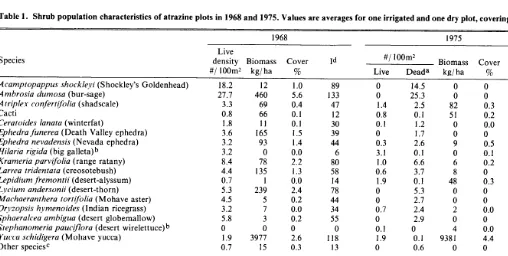
The pinyon-juniper sites supported a total living cover of 26.8%, while the true mountain mahogany sites hadonly 12.8% cover. True mountain mahogany had an average density of

1,225 plants/ha. Utah juniper averaged 382 plants/ha while pinyon pine averaged 62 plants/ha in the pinyon-j

Jn

iper type. Eighty-one species of plants were identified from t e study area. These included 2 trees, 18 shrubs, 51 forbs, and 10 grasses. Table 2 lists the most important species and their frequency values in the two communities. As can be seen, overall frequency values are low, indicating the general sparseness of vegetative cover on the sites.

Pinyon pine and Utah juniper trees were found in every study plot and were universally present throughout the study area. Average juniper tree density for the true mountain mahogany sites was 207 trees per ha, while the pinyon-juniper sites averaged 382 trees per hectare. Pinyon pine, however, ex- hibited greater density in the true mountain mahogany sites averaging 100 trees/ha and only 62 trees/ha in the pinyon- juniper type. This difference is partially explained in that 11 out

of the 20 mountain mahogany study sites had pinyon pine seedlings growing beneath true mountain mahogany shrubs. The deeper soil and modified habitat around the shrubs ap- parently provided a route for pinyon tree invasion. Seedling juniper trees were also observed growing beneath true mountain mahogany shrubs. True mountain mahogany sites appear to provide an avenue for the establishment of pinyon and juniper, on shallow soil within slickrock areas.

Evidence for true mountain mahogany preference for slick- rock areas is shown by a 16% mean cover value for rock in these communities, as compared to a 3% mean cover value for rock in the pinyon-juniper areas. Average density of true mountain mahogany in the relatively rock-free pinyon-juniper com- munities was 32 shrubs/ha, while on the rocky true mountain mahogany sites there was an average of 1,225 shrubs/ha. Thus true mountain mahogany communities dominate the harsh slick- rock sites and may be important in long-term successional changes in this area.

The two communities differed slightly in mean number of plant species per .04 ha. True mountain mahogany sites averaged 15 species per .04 ha, while the pinyon-juniper sites averaged 17 species. However, when a Shannon-Weaver diver- sity index (Shannon and Weaver 1949) was calculated for the plant cover of each type, true mountain mahogany had an average diversity value of 0.30, while the pinyon-juniper type had an average value of 0.23. This indicates a slightly more diverse plant cover in the mountain mahogany type. The lower value for the pinyon-juniper type reflects the dominant in- fluence of the trees.

There were differences in the species of plants found within the two types. Eleven plant species occurring on the pinyon- juniper sites were not found on the mountain mahogany sites. Also, nine species found on the mountain mahogany sites were not observed in the pinyon-juniper sites. Similarity indices (Ruzick 1958) were computed among all sites studied in the two types. The true mountain mahogany sites showed an average internal similarity index of 27.2, while the pinyon-juniper sites had an average of 35.4. When all mahogany plots were compared with all pinyon-juniper plots, an average similarity index of 20.9 was obtained. The larger the index value, the more similar the vegetative samples are; conversely, the smaller the index value, the more heterogenous is the sample. It is apparent that the pinyon-juniper community is internally more similar than the mountain mahogany community. The two communities are quite dissimilar with regards to each other.

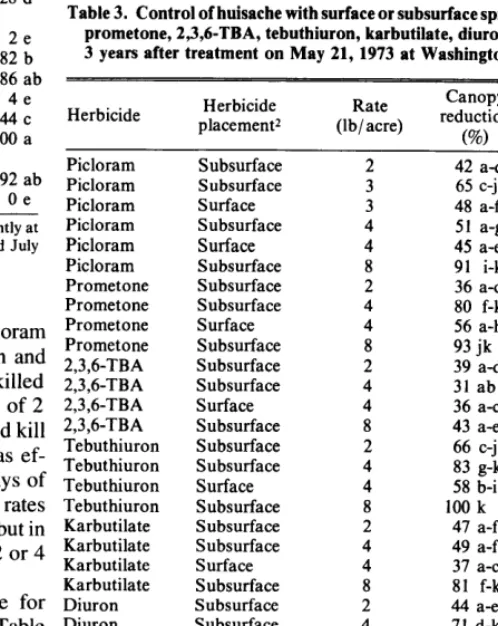
Analyses of growth form showed important differences between pinyon-juniper and true mountain mahogany vegeta- tions. Plant species were placed in five growth form groups: trees, shrubs, perennial forbs, perennial grasses, and annuals. Relative cover and frequency values were used for Chi-square analysis (Table 3). Based upon cover, there is a significant difference (P < 0.001) in the distribution of growth forms among the two communities. Frequency data also indicated a significant difference (P < 0.01) between the pinyon-juniper and the mountain mahogany sites. The pinyon-juniper type is a tree-annual forb association while the true mountain mahogany type is best characterized as a shrub-grass association.

A total of 100 mountain mahogany stems were aged by growth rings. If one ring equals a year, the stems ranged from 5 to 54 years old, with diameters ranging from 2 to 26 mm. Ring counts were significantly correlated (J’ < 0.001) with stem Table 3. Community

frequency.

growth form data in terms of relative cover and

Life Form

Cover Frequency

Mt. mahogany Pin.-June. Mt. mahogany Pin.-Jun.

Tree 42 80 13 19

Shrub 41 13 34 16

Forb 1 1 10 11

Grass 13 4 20 13

Annual 3 2 24 41

Total 100 100 100 100

diameter and plant height.

Size class data suggest that 90% of the mountain mahogany shrubs and Utah juniper trees in, the study area are mature or decadent. Only 10% of the individuals belonging to these two species were classed as seedling or young plants, indicating very little reproduction. Pinyon pine trees, however, showed good reproduction, with 35% of the individuals being classed as seedlings or young plants.

In the mountain mahogany sites (see Table l), soil depth beneath the plants (1.9 cm) was significantly deeper (P < 0.05) than the soil depth between the plants (1.3 dm). The pinyon- juniper type also showed significant differences (P < 0.001) beteen soil depth beneath the plants (2.8 dm) and soil depth between the plants (2.3 dm).

Percent sand as slightly greater in pinyon-juniper study sites, while percent clay and percent silt were both greater in soils of the mountain mahogany study sites.

Average pH values for the soils from between the plants of the true mountain mahogany type was 7.7, while the pH of the corresponding class of pinyon-juniper soils was 7.6. Soil from beneath plants showed pH values significantly ‘(PC. 0.001) more alkaline under mountain mahogany (7.9) as opposed to pinyon or juniper trees (7.7). Lower pH under pinyon-juniper trees is apparently due to the acid-forming needles and their resultant influence on the soil.

Soluble salt concentrations also exhibited interesting re- lationships in the two communities. In true mountain mahogany study sites, soluble salts are significantly (P < 0.05) less in soil from beneath shrubs than in soil from between shrubs. In the pinyon-juniper communities, a reverse situation occurred, with soluble salts being significantly (P < 0.001) greater in soil beneath pinyon and juniper trees than in soil between trees. These differences may be explained in several ways. The deeper soils beneath the shrubs may allow for deeper leeching; thus taking the critical ions beyond the depth of our sample. True mountain mahogany shrubs may absorb the soluble salts and incorporate them into their stems and leaves. Leaves are shed each year and seldom remain in and around the plants because winds tend to blow them away. Soluble salts contained in the leaves would thus be removed from the site. Other losses would most likely occur through the utilization in summer and winter of leaves and stems by deer. Thus, a gradual depletion of soluble salts from the soil beneath the mountain mahogany shrubs may occur.

The pinyon-juniper sites are located back from the windy edges of slickrock areas. Large pinyon and juniper trees act as

windbreaks, which collect blowing sand and organic material. Soluble salts would also be taken up by these plants into their vegetative parts. Leaves are continually shed, forming a thick layer of duff. Soluble salts contained in this duff are returned to the soil through the process of degradation and leaching. Thus, the salts in and around the trees are cycled from soil to tree, and back to soil again. The canopy and accumulated litter layer of pinyon and juniper trees also limits the amount of leaching that takes place in the soil beneath them. Precipitation reaching the soil beneath these trees is thus reduced and less leaching of the soil would be expected. Loss of soluble salts through wildlife feeding on the pinyon and juniper trees would be minimal.

Literature Cited

Anderson, D. L. 1974. Ecological aspects of Cercocarpus monranus Raf. com- munities in central Utah. Unpublished MS Thesis, Department of Botany and Range Science, Brigham Young University, Provo, Utah. 84 p. Beers, T. W., P. E. Dress, and L. C. Wensel. 1966. Aspect transformation

in site productivity research. J. Forestry 64:691-692.

Bouyoucos, G. J. 1951. A recalibration of the hydrometer method for making mechanical analysis of soils. J. Agron. 43:434-438.

Brooks, A. C. 1962. An ecological study of Cercocarpus montanus and ad- jacent communities in part of the Laramie Basin. Unpublished MS Thesis, Department of Botany, University of Wyoming, Laramie. 53 p.

Christensen, E. M. 1964. Succession in a mountain brush community in Central Utah. Proc. Utah Acad. of Sci. Arts and Letters 41(1):10-13. Daubenmire, R. 1959. A canopy-coverage method of vegetational analysis.

Northwest Sci. 33:43-46.

Martin, F. L. 1950. A revision of Cercocarpus. Brittonia 7:91-l 11. Medin, D. E. 1960. Physical site factors influencing annual production of true

mountain mahogany, Cercocurpus monranus. Ecol. 41:454-460.

Nie, H. H., C. H. Hull, J. G. Jenkins, K. Steinbrenner, and D. H. Bent. 1975. Statistical Package for the Social Sciences, second edition. McGraw- Hill Book Co., Inc., New York, N.Y. 675 p.

Nixon, E. S. 1977. A mountain Cercocarpus population-revisited. Great Basin Natur. 37:97-99.

Plummer, A. P. 1969. Restoring big-game range in Utah. Pub. No. 683. Utah Div. of Wild]. Resources. 183 p.

Pyrah, G. L. 1964. Cytogenetic studies of Cercocarpus in Utah. Unpublished MS Thesis, Department of Botany, Brigham Young University, Provo, Utah. 80 p.

Russell, D. A. 1948. A laboratory manual for soil fertility students, third edition. Wm. Brown Co., Dubuque, Iowa. 56 p.

Ruzicka, M. 1958. Anwendung Mathematisch. Statisticher Methoden in der Geobotanik (Synthetische bearbeitung von aufnahmen). Biologia, Bratisl 13647-661.

Shannon, C. E., and W. Weaver. 1949. The mathematical theory of com- munication. University of Illinois Press, Urbana. 65 p.

Soil Conservation Service. 1971. Plant handbook. Portland, Oregon. 100 p. U.S. Forest Service. 1937. Range plant handbook. U.S. Dep. Agr. U.S. Govt.

Printing Office, Washington, D.C. 120 p.

Effects of Predator Control on Angora Goat

Survival in South Texas

FRED S. GUTHERY AND SAMUEL L. BEASOM

Highlight: Predator control was conducted in South Texas during January-July 1975 and 1976 to determine its effects on productivity and survival of Angora goats. The control effort, when compared to an area receiving no treatment, reduced activity of coyotes and bobcats by 80%. Predators, mainly coyotes, killed 33 and 16% of the known kid crop on untreated and treated pastures, respectively. Because predators apparently were responsible for most unknown losses, the true predation loss was as high as 95 and 59%, respectively, of the known kid crop. The net kid crop under intense predator control was 27 times greater than that under no control, but the crop under treatment was only 13.5% because predation losses were still high. Coyotes killed 49 of 204 nannies (91% of losses) in an untreated pasture. They killed none in a treated pasture, but 10% of 205 nannies succumbed to nonpredator mortality. The data indicate that, in regions of high coyote density, intense localized predator control with traps, snares, and M-44’s could curtail predation on adult goats, but would be insufficient to prevent heavy losses of kids.

Cain et al. (1972) stressed the need for objective quantification of predation losses in domestic livestock, particular- ly sheep. Sanyal ( 1975) reported preda- tors killed 0.4 to 1.4% of the ewes and 1.4 to 2.5% of the lambs on two ranches in South Texas. In California, coyotes (Canis Zutruns) and other predators killed an estimated 40,400 sheep in 1973-74 (Nesse et al. 1976). Dorrance and Roy (1976) found sheep losses to predation averaged 1.6% of ewes and 2.8% of lambs in Alberta. On a ranch without predator control in New Mexico, predators (mainly coyotes) killed 15.6and 12.1%ofthelambcrop in 1974 and 1975, respectively

(DeLorenzo and Howard 1976). A

similar study in Montana reported predation losses of 8% of ewes and 29% of lambs during a l-year period in which predator control was practiced during the first 7 months (Henne 1975). Klebenow and McAdoo (1976) verified a predation loss of 4% for sheep in Nevada. It is now clear that coyote predation presents an economic prob-

Authors are instructor and associate professor, De- partment of Wildlife and Fisheries Sciences, Texas A&M University, College Station 77843. Guthery’s current address is Department of Range and Wildlife Management, Texas Tech University, Lubbock 79409. The study was approved by the Director, Texas Agr- cultural Experiment Station, as TA 13381.

The study was supported by the Texas Agr. Exp. Sta. and the Caesar Kleberg Res. Program in Wild]. Ecol. J. Williams, R. FOX, and D. Nobles aided in field work. Mr. and Mrs. J. Lee granted permission to conduct the study on their ranch. Drs. F. E. Smeins and W. G. Swank critically reviewed the manuscript.

Manuscript received May 5, 1977.

lem in the United States (Connolly et al. 1976).

Cain et al. (1972:47) also noted “there has been essentially no research aimed at determining the effectiveness of control methods in affecting the magnitude of predation losses.” Data interpreted by Wagner (1972) sug- gested that predation losses of sheep might be compensatory, to some ex- tent, with other types of losses on western ranges. If nonpredator mortali- ty increases in the absence of predation, predator control would be of questiona- ble utility in enhancing survival of these animals. Experimental analysis of the efficacy of predator control has yet to be done.

Although predation on sheep is clearly a problem, no studies have quantified the importance of predation in mortality of Angora goats, which was the first objective of the present work. The second was to determine the efficacy of predator control in reducing Angora mortality.

Study Area and Methods The study was conducted during January- July 1975 and 1976 in northern Zavala County, Tex . , in the South Texas Plains. Gould (1975) described the vegetation of this region and Tanner (1976) detailed the physical environment near the study area. Guthery (1977) described the study area, which supported dense stands of white- brush (Aloysiu fycioides), blackbrush acacia (Acacia rigid&), guajillo (A. berlundieri), and other species. Predomi-

nant grasses were threeawns (Aristidu spp.), common curlymesquite (Hiluriu belungeri), red grama (Boutelouu trifidu), buffalograss (Buchloe ductyloides), and pink pappus (Puppophorum bicolor).

Survival and productivity of Angora goats were compared between a 225ha treated (predator conrol) and a 201-ha un- treated (no predator control) pasture. The untreated pasture was separated from treated portions of the study area by 7 km. Mammalian predators were killed on a 1,550-ha area which included the treated pasture and a 1.6-km buffer zone on three sides of it. Trespass restrictions prevented establishment of a buffer zone on the fourth side. Steel leg-hold traps, M-44’s, and snares were deployed at an average intensi- ty of 20.4 device days/ha/month in 1975, where a device day is one device operative for 24 hours. In 1976 the intensity of mechanical control was 12.5 device days/ ha/month. About 1 hour of helicopter gunning was also conducted in February each year, and 6.2 hours of predator calling was done in 1975. Guthery and Beasom (1977a) described the predator control in greater detail,

Scat counts were conducted on 12.8- and 20.0-km routes in treated and untreated portions of the study area, respectively, to determine the effectiveness of the control in reducing predator activity. Scats were cleared from the two routes on 2 successive days, and the routes were run alternately over the next 4 days. In 1975 scats were not counted when the routes were cleared. In 1976 they were counted because rain hampered completion of the work. Only coyote and bobcat (Lynx rufus) scats, identified by Murie’s (1954) criteria, were used to compute scats/l .6 km, the activity index.

Prior to release onto the experimental pastures, each goat was weighed, measured around the girth, drenched for internal parasites, and tagged with individually numbered punch-through ear tags. Weight in kilograms divided by girth in centimeters times 10 was computed as an index of condition. Goats were examined super- ficially for physical deformities and general health.

After release the flocks were observed and counted daily except during rainy weather. Data were recorded on morbidity and reproductive condition. Pregnancy was

determined by the size and tightness of udders, by the size and shape of the abdomen, and by evidence of birth such as blood in the ano-genital region. The ear tag number of does with kids was recorded whenever families were seen together. The natural diet of the flocks was supplemented at a rate of 0.23 kg corn/ goat/day from the early February release through mid-March. Besides enhancing productivity, this gentled the flocks for observations and counts.

Carcass searches on foot and horseback were conducted when counts indicated goats were missing. During 1975 and 1976 combined, 262 and 351 hours were spent searching in the treated and untreated pastures, respectively. The average search intensity was 6 and 12 minutes/ha/month, respectively. These figures understate the effective search intensity because (I) con- siderable time was spent in the pastures doing other work, (2) searches were not conducted in all months in the treated pasture because no mortality was occurring, and (3) searches were concentrated on portions of the pastures used by goats. Field necropsies were conducted when carcasses were found. Predation was as- signed as the cause of death following criteria described by Anderson (1969), White (1973), and Bowns (1976).

Results and Discussion Predator Control

Sixty-nine coyotes, 11 bobcats, and 52 smaller mammalian predators were killed on the treatment area in 1975. Comparative figures for 1976 were 63, 7, and 32, respectively.

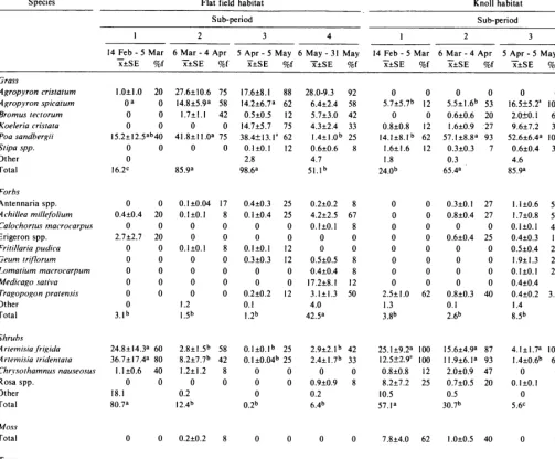
Predator control apparently reduced the presence of major predators (coyo- tes and bobcats) because the activity index invariably was lower on the treat- ment area (Fig. 1). Over the study period, the average activity index on the treatment area was about 80% lower than that of untreated areas. Guthery (1977) calculated that in 1975 late winter density of major predators on the treatment area was about 0.8/km2, which compared to about 2 .O/km” on untreated areas. Presence of sign indi- cated the treatment area was never free of major predators, but density ap- parently dropped to about 0.4/km2. Based on catch data, coyotes were roughly six times more abundant than bobcats. Thus the predator control reduced coyote density from high

South Texas levels (Knowlton 1972) to levels typical of many portions of the West (Wagner 1975).

Homogeneity of Experimental Flocks The experimental flocks were tested for homogeneity between pastures

2

r - - - -

Untreated

Treated

1

0

FMAM

JMA

MJ

1975

MONTH

1976

Fig. 1. Comparative activity of major predators (coyotes and bobcats) on untreated (no predator control) and treated areas, Zavala County, Texas.

because extrinsic sources of variation could affect productivity and survival independent of predation. The produc- tivity of Angora does, for example, tends to vary directly with weight with- in and among age classes (Shelton and Stewart 1973). Results of t tests indi- cated the mean weight and girth were similar (P>O.O5) between treatments within years, suggesting the desired homogeneity was realized.

Different pregnancy rates or differ- ent parturition periods associated with different weather patterns also could influence comparative kid survival independent of predation. Contingency tables were therefore constructed to examine frequency distributions of reproductive parameters. The nannies, by pastures, were cross-classed with pregnancy status (pregnant, barren, unknown), live kid status (one, two, none), and weight class of adults in 2.27-kg intervals. None of the resulting Chi-square values was significant (P>O.O5), again suggesting homoge- neity .

Productivity and Survival

Barren nannies were an important cause of lowered productivity. In 1975, 84% of the untreated nannies were pregnant, 5% were barren, and 11% were of undetermined pregnancy. Re- spective figures for the treated flock were 93,4, and 3%. In 1976 50% of the untreated nannies were pregnant, 41% were barren, and 9% were of undeter- mined pregnancy. Respective figures for the treated flock were 54, 29, and

17%. The lower fertility rates of 1976 possibly were due to drouth conditions for 5 months preceding kidding. Be- cause we made special efforts to identify

nannies with tight udders or signs of parturition, most nannies of undeter- mined pregnancy likely were barren. Moreover, evidence of the bleeding associated with birth was detectable on hindquarters for up to a month. Com- bined over both flocks and years, these data suggest a 70% pregnancy rate in the experimental flocks.

Table 1. Partitioned losses of the known Angora kid crop on untreated (no predator control) and treated pastures during February-July, Zavala County, Tex.

Source of loss

Unknownh Predation Starvation or

abandonment UndeterminedC Stillborn Unknown,

not predation Infection, trap wound Congenital deformation

Subtotals Kids survived

1975 1976

(601a (29)

35 19

21 8

Untreated Treated

Total % of % of 1975 1976 Total % of % of

(89) kid crop losses (63) (37) (100) kid crop losses

54 62 62 18 25 43 43 59

29 33 33 14 2 16 16 22

1 1 I 1 2 5 7 7 10

2 2 2 2 2 I 3 3 4

1 I 2 2 2 1 I 1 1

1 1 I I

1 1 1 1

1 1 1 1

59 29 88 99 40 33 73 73

I 1 1 23 4 27 27

aKnown minimum number of kids born. bDisappeared without trace.

CCarcass fragments too old.

be additive rather than compensatory. Ninety-seven kids seen alive dis- appeared without trace, resulting in the preponderance of unknown losses in both pastures (Table 1). Because (1) predation was responsible for over 50% of known losses, (2) survivorship was higher where predators were being destroyed (Fig. 2), and (3) coyote scats composed of mohair appeared on the study area concurrent with the dis- appearance of kids, it was apparent that kids were disappearing under predator pressure. Predation should be suspected when animals suddenly vanish and leave no trace (Robinson 1952), be- cause, for example, a coyote can kill and consume a white-tailed deer

(Odocoileus virginianus)

1964). Klebenow and McAdoo ( 1976) also suspected coyote predation when domestic lambs vanished in their Nevada verification study; they found only the ear of one lamb near a coyote den. Thus predators were probably responsible for most unknown losses in this study, a conclusion strengthened by the fact that disease or other abnormalities rarely were noted among the kids during frequent observations of the flocks. Predator losses therefore accounted for 33 to 95% (33 to 95% of losses) and 16 to 59% (22 to 8 1% of losses) of the known kid crop on the untreated and treated pastures, respec- tively. The true predation loss ap- parently fell on the higher

extremes of

that predators apparently were respon- kidding in well-protected areas, and sible for most kids lost in the treated holding kids in these areas until about 2 pasture; a more effective control weeks of age, is a possible cultural regime would have increased the kid practice for decreasing the severity of

crop there. predation problems.

The effect of predator control on kid survival was most noticeable 6 to 7 days after birth. During the first week of life, kid mortality was high in both pastures (Fig. 2). This indicates that

Predation on nannies was less severe than that on kids. Coyotes killed three nannies in 1975 while the flocks were being held in a 32-ha pasture prior to release, but none was killed on the

1975

80

Be- Untreo

ted

60

Intensive predator control increased the kid crop by 2,700% in this study. Because the kid crop was only 13.5% under treatment, the former figure is less impressive. Recognize, however,

20

40

DAYS AFTER BIRTH

Fig. 2. Forty-day survivorship of Angora kids in untreated (no predator control) and treatedpastures, Zavala County, Texas.

Table 2. Partitioned losses of adult Angora goats on untreated (no predator control) and treated pastures during January-July, Zavala County, Tex.

Untreated Treated

1975 1976 Total % of % of 1975 1976 Total % of % of

Source of loss (102)a (102) (204) flock losses (103) (102) (205) flock losses

Predation 49b 49 2’: 91

Meningeal worm 1 1 2 16e I6 8 76

Unknown,

not predation 3 3 1 5 1 I 2 <l 9

Bogged in mud 1 1 1 2

Ear tumor 1 1 <l 5

Screw worm I 1 <1 5

Unknown 1 1 <l 5

Subtotals 1 53 54 26 17 4 21 10

Adults survived 101 49 150 74 86 98 184 90

aNumber of goals stocked.

hIncludes two nannies that died from infection of coyote wounds and five whose carcasses were old. but showed evidence, both direct and circumstantial, of predation.

c Includes eight nannies removed for diagnostic examination before death. dDiagnosis not confirmed by laboratory examination of larvae.

experimental pastures (Table 2). In 1976 predation on nannies was heavy in the untreated pasture and was, there- fore, the major source of mortality in the flock over the 2 years.

Meningeal worm (Parelaphostron-

gylus tenuis) infection lowered survival of nannies in the treated pasture in 1975 (Fig. 3) and was responsible for most of the 10% overall death loss. The infection should not be regarded as a compensating loss factor, however, because the infection rate in the untreated pasture (4.8%) was lower, rather than equal to, that in the treated pasture (22%).

Over the 2 years, nanny survival under treatment was 122% of that with no treatment. The data indicate that, under relatively intense predator con- trol with mechanical methods, nannies could be pastured in regions of high coyote densities with little mortality from predation.

Factors Influencing Predation Rates Because predation losses tend to vary directly with coyote density (Wagner 1975)) higher coyote numbers in 1976 possibly would explain the heavier predation on both kids and nannies that year. This appears to be an unlikely explanation. The coyote kill in January and February, standardized to number caught per 1,000 snare plus 1,000 trap days, was 2 1.3 (1975) and 19.3 (1976), which suggests similar densities in the 2 years.

Decreased buffer prey can induce increased predation on livestock (Gier 1968) and may have played a role in the increased predation rates of 1976. Although lagomorph and deer densities were essentially equal both years, mean rodent densities declined (Table 3) by about 58 and 29% in the untreated and

treated pastures, respectively, in 1976. Rodents, especially cotton rats (Sig-

modon hispidus) and woodrats (Neo-

toma micropus), the most abundant species on the study area (Guthery 1977), are important in the diet of South Texas coyotes (Knowlton 1964; Sanyal 1975; Brown 1977).

An apparent relation between month of birth and kid survival partially explains the difference observed be- tween years. To examine this relation, the percentage of the first 30 days of life survived was determined for each kid. The means over both pastures and years were 17.5 (n=42), 29.7 (n=61), 48.1 (n=58), and 33.9% (n=9) in February, March, April, and May, respectively. A null hypothesis about these means

was

points

trend

ruary through April and a decline in May was similar in both pastures. In 1975 47, 47, and 6% of the kids were born in March, April, and May, respec- tively. In 1976,74, 14,9, and 3% were born in February, March, April, and May, respectively. Thus in 1975 more births occurred in later months when more predators had been removed from the treated area. Because survival on the untreated pasture showed similar trends, however, other factors were operating. During 1975, densities of rodents and cottontails (Sylvilagus

floridanus) rose steadily from January through July in the untreated pasture (Guthery and Beasom 1977b). These increasing buffer prey populations may have ameliorated predation on kids as the study progressed. By virtue of

greater numbers, 1975 kids had

stronger influence on the 2-year mean percentages in this pasture.

Table 3. Densities (number/40 ha) of animal prey and fruit-producing shrubs to compare availability of natural foods for predators between untreated (no predator control) and treated pastures, Zavala County, Tex. The data are from Guthery and Beasom (1977b) and Guthery (1977).

Species

1975a l976h

Untreated Treated Untreated Treated

All rodents Cottontails

(Sylvilagus floridanus) White-tailed deer

(Odocoileus virginianus) Jackrabbits

(Lepus californicus) Mesquite

(Prosopis glandulosa) Pricklypear

(Opuntia sp.) Persimmon

(Diospyros texana) Condalias

(Condalia spp.) Granjeno

(Celtis pallida)

704 416 296 296

49.7 22.0 49.5 43.0

1.8 5.1 2.6 4.1

<2 (2 <2 <2

560 13,120 2,400 8,320 5,680 2,400 3,280 6,440 9,880 8.320 a Animal densities are January-July averages.

Table 4. Least squares analysis of variance of kid survival, Zavala County, Tex. The classifi- cation variables are year (1975, 1976), pasture (untreated, treated), and birth month (February, March, April, May). The dependent variable was the percentage of the first 30 days of life survived.

Source of

variation df MS F P>F

Model 8 7S90.8 5.85 0.000 1

Year 1 220.6 0.17 0.6807

Pasture I 14,024.4 10.81 0.0012

Birth month 3 3,254.3 2.52 0.0592

Birth month by pasture 3 2,000.4 1.54 0.2044

Error 161 1,297.8

A minimum of 123 kids was born in 1975 compared to 66 in 1976 (Table 1). Death of a kid in 1976 was roughly twice as important, in terms of percent- ages, thereby influencing portrayed survivorship (Fig. 2) disproportionate- ly. This condition, sometimes called small-sample bias, also should be recognized when interpreting cause of loss as a percent of flock (Tables 1 and 2).

The larger number of kids born in 1975 (Table I), whose births were more evenly distributed in time, may have buffered predation on nannies in this year. No nannies were killed in the untreated pasture while kids survived.

A last factor possibly contributing to increased predation rates in 1976 in- volved historical (Holling 1965) or learned aspects of predation. When introducing goats into a new area, ranchers in South Texas have reported moderate predation losses the first year and substantial losses the second. Although ecological factors such as buffer prey abundance were unknown in these instances, the phenomenon seems general and predictive enough to warrant consideration. Perhaps preda-

tors undergo some form of habituation to vulnerable livestock, or perhaps they build traditions by killing kids, sub- sequently killing adults, and then training the young.

Coyote Predation on Angoras

That coyotes were responsible for most, if not all, of the predation losses was evident from sign at kill sites. Coyote tracks and/or droppings, sever- al composed of mohair, usually were found within a few meters of carcasses. Most killing took place where past observations of tracks indicated heavy coyote use. None of the carcasses was covered with material or brushed to- gether as is characteristic of bobcat predation (Cook et al. 197 1). Mature goats were attacked in the larynx region, typical coyote behavior (Bowns

1976; Connolly et al. 1976).

The killing of kids began almost as soon as they were born in 1975. This took place on a ranch where Angoras had not been stocked in nearly a decade, where buffer prey populations were substantial (Table 3), and where the nearest other flock was 16 km away. These observations suggest that Angora kids are readily predated by

naive coyotes, as is the case with coyotes and sheep (Connolly et al. 1976), and, by extension, indicate the problem-animal concept of predator control (Cain et al. 1972; Henderson

1972) would have little merit in protecting Angora kids in South Texas.

The location of killing was a function of goat behavior. When a nanny entered labor, the rest of the flock went about normal activities, eventually leaving her (unless the birth occurred on the bedgrounds). She usually stayed with the newborn 2 to 3 days, then left it “lying out” and returned to the flock. There was no apparent pattern for her to return and nurse the kid; one instance was recorded of a nanny leaving her kid for 37 hours before feeding it. After the kid reached 10 to 14 days of age, it was capable of traveling with the flock and often did. Occasionally nannies left a small group of kids unattended during daylight while the flock foraged. Most kids were killed during the critical first few days of life, before they joined the flock. Their location during this time was largely a matter of chance, de- pending primarily on the habits of the flock and secondarily on where the nanny entered labor.

Adult goats generally were. killed on or near the bedgrounds, which were evidenced by an accumulation of fresh droppings and an odor of urine. On one occasion, tracks indicated coyote(s) ran a goat for about 300 m before killing it. Goats move upwind to bed down and usually mass as one flock. Thus they usually bed on the periphery of a pasture, which aided our carcass searches because about 80% of the kills were within 40 m of ranch roads

\

m \

--- \

\

0 \

ii

80 - 80 _ \

Untreated \

--- - _\

5 Treated -\ \ _L

5 60,

.\ \ _\

z

1975 60 _ 1976 .\ _-I

Z

-L

ii

\ -Z

/:

!e

j

4:

MAR 1 APR I MAY I JUN I FEB MAR I APR MAY I JUN ,

I I I I I I I I e I I I I I I I I

0 40 80 120 160 0 40 80 120 160

DAYS EXPOSED TO PREDATION

Fig. 3. Survivor-ship of adult Angora goats in untreated (no predator control) and treated pastures, Zavala County, Texas.

surrounding the untreated pasture. Nine nannies survived apparent coy- ote attacks during the study. Four were lacerated in the throat, five in the flanks or hams. Four nannies were attacked on a night when three others were killed.

Coyotes selected the youngest, smallest kids before older kids and kids before nannies. Nannies were not killed in 1976 until the last kid was lost and predation on adults began almost im- mediately.

Whether coyote predation on adult goats was selective for inferior individ- uals cannot be determined unless the proportions of healthy and debilitated animals in the flock are known. Formal records of these proportions were not maintained. Nonetheless, the kill in- cluded five nannies weakened from previous coyote attacks (health prior to attack was unknown), three slightly crippled, one in poor condition and suffering diarrhea, and one with a broken hock (old injury) that impaired her running ability. Thus 20% of the

kill was composed of somewhat

debilitated animals. Behavioral aber- rancies, such as separating from the flock due to illness or injury, apparently made goats highly susceptible to preda- tion because killing occurred in the three known instances of this behavior in 1976. Whereas coyotes took both the healthy and the infirm, some selection for the latter seemed likely. This conclusion is supported by the fact that the pre-experiment condition index of the 49 nannies killed was lower (PcO.01) than that of the 49 nannies surviving in the untreated pasture in 1976. Whether the index truly reflects condition is open to speculation, but girth would be more stable than weight and the index should vary directly with a nanny’s health and nutritional state, though perhaps not linearly. Regard- less of the validity of the index, the mean weight (2.83 kg heavier in survivors) and girth (2.4 cm larger in survivors) were significantly different (P<O. 0 1 ), indicating coyote selection for smaller nannies.

Whereas the condition index was determined from measurements of girth and weight, it may seem redundant to examine each separately. The index, however, is a variable that adjusts for differences in body structure. Had coyotes been selecting solely for smaller animals, the condition indices, according to normal theory, would have been equal. That they were not

suggests selection for both large and small animals in poorer condition; smaller animals probably were select- ed, to some extent, independent of condition.

Conclusions

In the absence of catastrophic losses due to cold rainy weather or similar factors, coyote predation apparently is the major source of mortality to range flocks of Angora goats in South Texas. In addition, the data indicate intensive predator eradication with traps, snares, M-44’s, and shooting can substantially increase the survival of kid and adult goats in this region, but is insufficient to curtail large losses of kids to predation, at least when conducted on a small scale and when total eradication of coyotes is not attained. It follows that predation losses of Angoras are, at most, slightly compensatory under low stocking rates and proper husbandry.

We should recognize, however, that Angora goats are inherently subject to a number of problems which tend to decrease their productivity and increase their mortality under range conditions. A weak mothering instinct (Gray and Groff n.d.; this study) a problem with udder deformities (Shelton and Stewart 1973; this study) poor reproductive performance under nutritional stress (Huston et al. 197 1 ), and an intolerance of cold wet weather after shearing make large losses possible in a total absence of predators. Thus predator control emerges as a valuable adjunct to, but certainly no substitute for, proper range management and animal husbandry.

Literature Cited

Anderson, T. E. 1969. Identifying, evaluating, and controlling wildlife damage. In: R. H. Giles (Ed.) Wildlife Management Techniques. Wildlife Society, Washington, D.C. p. 497- 520.

Bowns, J. E. 1976. Field criteria for predator damage assessment. Utah Sci. 37:26-30. Brown, K. L. 1977. Coyote food habits in

relation to a fluctuating prey base in South Texas. MS Thesis. Texas A&M Univ., Col- lege Station. 60 p.

Cain, S. A., Chairman. 1971. Predator con- trol-l 97 1. Institute for Environmental Quali- ty, Univ. of Michigan, Ann Arbor. 207 p. Connolly, G. E., R. M. Timm, W. E. Howard,

and W. M. Longhurst. 1976. Sheep killing behavior of captive coyotes. J. Wild]. Manage. 40:400-407.

Cook, R. S., M. White, D. 0. Trainer, and W. C. Glazener. 1971. Mortality of young white-tailed deer fawns in South Texas. J. Wild. Manage. 35147-56.

DeLorenzo, D. G., and V. W. Howard, Jr. 1976. Evaluation of sheep losses on a range

lambing operation without predator control. Final Rep. to the U.S. Fish and Wild]. Serv., Denver Res. Center, Colo. 34 p. (multilithed). Dorrance, M. J., and L. D. Roy. 1976. Preda-

tor losses of domestic sheep in Alberta. J. Range Manage. 29:457-460.

Gould, F. W. 1975. Texas plants-a checklist and ecological summary. Texas Agr. Exp. Sta. Misc. Pub. 585 (Rev.). 121 p.

Gray, J. A., and J. L. Groff. n.d. Texas Angora goat production. Texas Agr. Exp. Sta. Bull. 926. 18 p.

Guthery, F. S. 1977. Efficacy and ecological effects of predator control in South Texas. PhD Thesis. Texas A&M Univ., College Sta- tion. 50 p.

Guthery, F. S., and S. L. Beasom. 1977a. Effectiveness and selectivity of neck snares in predator control. J. Wild]. Manage. 42: In Press.

Guthery, F. S., and S. L. Beasom. 1977h. Re- sponses of game and nongame wildlife to predator control in South Texas. J. Range Manage. 30404-409.

Henderson, F. R. 1972. Controlling coyote damage. Kansas Coop. Ext. Serv. Bull. C-397. 24 p.

Henne, D. R. 1975. Domestic sheep mortality on a western Montana ranch. MS Thesis. Univ. of Montana, Missoula. 53 p.

Helling, C. S. 1965. The functional response of predators to prey density and its role in mimic- ry and population regulation. Mem. Entomol. Sot. Canada 45. 60 p.

Huston, J. E., M. Shelton, and W. C. Ellis. 1971. Nutritional requirements of the Angora goat. Texas Agr. Exp. Sta. Bull. 1105. 16 p. Knowlton, F. F. 1964. Aspects of coyote

predation in South Texas with special refer- ence to white-tailed deer. PhD Thesis. Purdue Univ. 189 p.

Knowlton, F. F. 1972. Preliminary interpreta- tion of coyote population mechanics with some management implications. J. Wild]. Manage. 34:369-382.

Murie, 0. 1954. A field guide to animal tracks. Houghton Mifflin Co., Boston. 374 p. Nesse, G. E., W. M. Longhurst, and W. E.

Howard. 1976. Predation and the sheep industry in California. Univ. of California Division of Agr. ti. Bull. 1878. 63 p. Robinson, W. B. 1952. Some observations on coyote predation in Yellowstone National Park. J. Mammal. 33:470-476.

Shelton, M., and J. R. Stewart. 1973. Parti- tioning losses in reproductive efficiency in Angora goats. /n: Texas Agr. Exp. Sta. Consolidated PR 3 179-3 19 1. p. 28-3 I. Sanyal, N. K. 1975. The effects of grazing

regime on coyote-sheep relationships in south- west Texas. MS Thesis. Texas A&M Univ., College Station. 64 p.

Tanner, G. W. 1976. Early effects of an 80% herbicide strip treatment on habitat use by white-tailed deer (Odocoileus virginianus) on the northern Rio Grande Plain, Texas. MS Thesis. Texas A&M Univ., College Station.

106 p.

Wagner, F. H. 1972. Coyotes and sheep: some thoughts on ecology, economics and ethics. 44th Utah State Univ. Faculty Ass. Honor Lecture. 59 p.

Wagner, F. H. 1975. The predator-control scene as of 1974. J. Range Manage. 28:4-10. White, M. 1973. Description of remains of deer

fawns killed by coyotes. J. Mammal. 54: 29 l-293.

Moisture and

Temperature

Requirements

Adventitious Root Development in Blue

Grama Seedlings

D. D. BRISKE AND A. M. WILSON

Highlight: The environmental requirements for adventitious

root initiation and growth in 22-day-old blue grama (Bouteloua

grucilis) seedlings were determined under controlled temperature and soil moisture conditions. The seminal root was maintained in moist soil; but surface soil (in which adventitious roots may develop) was independently maintained at various degrees of drought. Drought treatments were imposed by controlling the relative humidity of air above the soil and around seedling crowns. In the 100% humidity treatment, elongation rates of the longest root per seedling at temperatures of 15,20,25, and 30°C were 0.40, 0.74,1.04, and 1.22 cm per day, respectively. In the 96% humidity treatment, elongation rates at these temperatures were 0.28,0.36, 0.38, and 0.44 cm per day, respectively. When the seminal root is growing in moist soil, blue grama seedlings can initiate adventi- tious roots during severe drought conditions in the surface soil. However, adventitious root growth adequate for seedling estab-

lishment will probably not occur at moisture and temperature

conditions of less than 96% humidity (-50 bars) and 15°C.

Blue grama (Bouteloua grucilis) is the dominant perennial grass throughout much of the Great Plains. However, new seedlings are rare: in the past 40 years, workers at the Central Plains Experimental Range, in northeast Colorado, have failed to find natural reproduction of blue grama from seed (Hyder et al. 1975). Many attempts to establish plantings of blue gramaon the 5 million acres of abandoned cropland in the Central Great Plains have failed (Bement et al. 1961; 1965).

Blue grama seedlings have a single short-lived seminal root. Therefore, seedling establishment requires the development and extension of adventitious roots (Esau 1960). In the field, seedlings failing to extend adventitious roots die at approxi- mately 6 to 10 weeks of age (Hyder et al. 1971).

The poor seedling success of blue grama has been related to its seedling morphology. Blue grama seedlings have a short coleoptile and an elongated subcoleoptile internode, which places the coleoptilar node and all tillering crowns, from which adventitious roots may arise, on or very near the soil surface (Hyder et al. 197 1). Consequently, seedlings often fail to develop adventitious roots because of rapid drying of the soil surface. Adventitious roots grow out of tillering crowns and become successfully established when damp, cloudy weather persists for 2 or 3 days (van der Sluijs and Hyder 1974).

The authors are, respectively, graduate research assistant, Department of Range Science, Colorado State University, and plant physiologist, U.S. Department of Agri- culture, Agricultural Research Service, Crops Research Laboratory, Colorado State Uni- versity, Fort Collins 80523. Briske currently is assistant professor, Dep. Range Science, Texas A&M Univ., College Station, Texas.

The study involved cooperative investigations of the Agr. Res. Serv., U.S. Dep. Agr., and the Colorado State Univ. Experiment Station, Fort Collins 80523. (Scientific Series Paper No. 2269.) The authors thank John A. Sarles for valuable technical assistance during this study.

Manuscript received October IO, 1977.

174

for

Olmsted (1941) recognized a similar situation with sideoats grama (Bouteloua curtipendulu). Elongation of the first inter- node (subcoleoptile internode) elevated the coleoptilar node to the soil surface or as much as 8 mm above it. He also observed that approximately three consecutive wet days were required for the successful establishment of adventitious roots. Hoshikawa ( 1969) examined three genera of the tribe Chlorideae and found them all to exhibit subcoleoptile internode elongation.

Adventitious roots are rapidly initiated and possess rapid growth rates, enabling them to become established during periods of adequate surface soil moisture. Initiation of the first adventitious root occurred when blue grama seedlings were 11 days old (van der Sluijs and Hyder 1974). Similar results have been observed with sideoats grama (Hopkins 1941; Olmsted

1942). When tillering crowns of 2 1 -day-old blue grama seedlings were exposed to moist soil, roots developed within a few hours (van der Sluijs and Hyder 1974). The average maximum rate of adventitious root growth was 3 cm in 24 hours. Briske and Wilson (1977) found a maximum elongation rate of 2.6 cm per day; Olmsted (1941), working with sideoats grama, reported an elongation rate of 2 cm per day.

Adventitious roots may fail to develop at low temperatures, even though moisture conditions at the soil surface are favorable (Briske and Wilson 1977). Therefore, we conducted an experi- ment to define the moisture and temperature conditions required for initiation and growth of adventitious roots. The experiment was designed to simulate field conditions in which the seminal primary root extends into moist soil but the seedling crown remains in contact with surface soil at various degrees of drought.

Methods

Blue grama seed of accessions PM-K-1482 and PM-K-1483 were obtained from the Soil Conservation Service, Manhattan, Kans. Accession 1482 is a synthetic blend of six accessions from the Central Plains (Nebraska and northern Kansas); accession 1483 is a synthetic blend of 12 accessions from the Southern Plains (southern Kansas and Texas). Each of the blends was produced by planting the accessions, from the respective regions, together in 1971 at the Plant Materials Center, Manhattan, Kans. Seed for this study was harvested in 1974.

Seed were planted at a depth of 2 cm in plastic pots (15 cm diameter by 15 cm deep) filled with autoclaved sandy loam soil. During seedling development in the greenhouse, the pots were subirrigated to promote growth of the seminal primary root and to maintain a dry surface soil layer of 1.5 cm that would prevent initiation of adventi- tious roots. At 22 days, soil was removed from the top of each pot to

expose the seedling crown and a portion of the subcoleoptile internode. A large plastic petri dish, with a small petri dish fastened within it, was placed over the seedling and fastened to the rim of the pot with latex calking compound (Fig. 1). The seedling protruded through a hole in