Travel time Reliability Analysis Using Entropy

(1)

Volume 4, No. 10, September-October 2013

International Journal of Advanced Research in Computer Science

RESEARCH PAPER

Available Online at www.ijarcs.info

ISSN No. 0976-5697

Travel time Reliability Analysis Using Entropy

Neveen Shlayan

Research Intern

Philips Research North America Briarcliff Manor, NY USA [email protected]

Vidhya Kumaresan*

Department of Civil and Environmental Engineering University of Nevada Las Vegas

Las Vegas, USA [email protected]

Pushkin Kachroo

Professor, Department of Electrical Engineering University of Nevada Las Vegas

Brian Hoeft

Director, Freeway and Arterial System of Transportation RTCSNV

Abstract: Travel time reliability is a measure that is commonly extracted from travel time measurements. It has served as a vital indicator of the transportation system’s performance making the concept of obtaining reliability from travel time data very useful. Travel time is a good indicator of the performance of a particular highway segment. However, it does not convey all aspects of the overall performance of the transportation system. Travel Time Reliability is defined as the consistency of traffic conditions on a given link. Predictability is desired since travelers tend to give a higher value to consistency of travel times rather than the pure travel time data. Previous studies have explored various analysis approaches for this purpose. Most commonly used methods are the traditional statistical methods demonstrating variability. A vital question to ask is how adequate these standard statistical quantities are. There are numerous measures of travel time reliability that look at how reliable the travel time measurements are from different perspectives. This paper presents an overview of the current methods of calculating travel time reliability and introduces a new approach by using the concept of entropy from information theory. The information theory based approach is demonstrated through failure analysis.

Keywords: Travel time reliability; Reliability Analysis; DMS Travel Times; Information Theory

I. INTRODUCTION

Travel time is the time that users of the roadway system take to commute from an origin to a certain destination. Considering a fixed length of a highway section, travel times directly reflect traffic conditions, such as congestion due to recurring or nonrecurring events. Traffic conditions caused by nonrecurring events are highly unpredictable causing unexpected delays which are automatically reflected in travel times. This uncertainty results in variable traffic conditions and is measured by “travel time reliability”. The uncertainty associated with travel times is of major importance to drivers and is highly ranked among all influential factors of departure time choice of travelers [1]. The inconsistency of travel times inflict a scheduling cost where commuters have to budget extra time when traveling a certain route [2]. Therefore, travel time reliability is an imperative measure in transportation system management [3].

Travel time reliability can take various quantitative measures all of which differ to a certain degree in the information they contain when evaluating the reliability of a route. The appropriate measure that ought to be chosen depends on the evaluation criteria. Most researchers as well as transportation entities use standard statistical methods when defining reliability. In this paper, in addition to the traditional reliability measures, an information theory based approach is proposed which adds an innovative dimension to the meaning of reliability. The objective of the use of information theory is to examine how consistent the data is as opposed to how good it is. Another concept of failure analysis using this information theory is also demonstrated.

The proposed reliability measures in addition to the traditional ones are applied on travel time data obtained from Dynamic Message Sign (DMS) on the Interchange 15 (I-15) in Las Vegas in order to demonstrate the differences. In short, this paper introduces the use of information theory in travel time reliability analysis in addition to introducing the readers to existing measures and their demonstration.

II. LITERRATURESURVEY

The importance of travel time reliability has been discussed by numerous studies. Tilahun and Levinson [4], Fosgerau and Karlstrom [5] and Small et. al [6] examine the value of travel time reliability for the users. Bogers in [1] recognized the various reliability measures that have been used and concluded that the reliability analysis method depends on the application. Nie and Fan [7] developed an adaptive routing strategy, named the stochastic on-time arrival (SOTA) algorithm, to target least-expected travel time as a mechanism to address the performance measure of reliability. Oh and Chung [3] studied travel time variability using data from Orange County, California. They studied travel time variability computed in terms of variance in day-to-day, within-day and spatial variability. They concluded that travel time is correlated with standard deviation. Chen et. al. [2] demonstrated the relationship between travel time and level of service. They showed how their 90th percentile travel incorporates the mean and variability into a single measure, and also studied how travel time information using ITS can reduce travel uncertainty.

(2)

reliability ratio which gives an assessment of the extra time commuters must account for based on variance [2]. Van Lint [10] defined skew as a measure of the asymmetry of the travel time distribution and claimed its importance in travel time reliability. Cambridge Systematics [11] used planning time, planning time index and buffer index to measure reliability and found that buffer and planning time indices are very useful statistical measures. Buffer index is defined as the extra time needed to accomplish a certain trip with respect to the mean travel time; whereas, planning time index is an indication of the deviation of the buffer size from the ideal travel time [11]. Buffer time index was also used by Mehran and Nakamura [12] to compare congestion relief schemes. Lomax and Schrank [13] used measures of reliability like travel time window, buffer time and misery index. The study also made recommendations on the type of measures that should be used for certain areas and modal combinations. The literature review clearly suggests that travel time reliability can take various measures and the optimal reliability approach choice is dictated by the examined aspect of the specific application. In this study, different reliability approaches consisting of traditional and new methods are used to analyze travel time data on the Interstate-15 Las Vegas area. Classical method, variability based on normalized standard deviation, Analysis of Variance (ANOVA), travel time mean estimation, reliability as a measure of non-failures and information theory based approaches are used and the results are compared.

III. RELIABILITYMEASURESANDTECHNICAL METHODS

The term “reliability” suggests repeatability or dependability. For a random experiment this would mean that the results of an experiment are repeatable. In terms of travel-time, if travel time is measured repeatedly on a section we get comparable values. In general, repeatability of travel time could be framed in terms of time-of-day, day of the week, etc. Thus, travel time reliability is determined by conducting analysis on data measured for a certain segment.

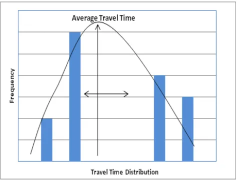
[image:2.595.319.557.53.233.2]

All of the traditional methods of measuring travel time reliability are extremely important in seeing how they measure reliability. But, it is also important to look at the data in an unbiased manner to understand the information that it contains. For example, in the following distribution, traditional measures of reliability would look at the mean and how far the observations lie from the mean.

Figure. 1. Travel time frequency distribution

The deviation from mean for the second plot will be higher than the first plot in Figure 1, according to the standard methods of reliability measurement. Whereas according to information theory, the information gained from both plots remain the same, since by definition; the entropy of the data is independent of the mean or the location about the mean. The methodology describes the current methods of measuring travel time reliability and proposes the use of information theory as an additional way of measuring a different aspect of reliability.

A. Classical Methods: Planning Time, Planning Time Index, Buffer Index:

Traditionally, reliability is measured through calculating the planning time (the buffer) and the two indices planning time index and buffer index through analyzing the travel time frequency distribution. Planning time or the buffer is calculated as the 95th percentile of travel time as demonstrated in Equation 1. The planning time buffer indicates the extra time travelers should account for in order to guarantee on-time arrival. Planning time index is the ratio of the planning time to the ideal travel time (free flow) which indicates how planning time compares to ideal travel time giving more information about how severe traffic conditions were. The sheer buffer size (planning time) indicates consistency of travel times. Buffer index is the ratio of the difference between planning time and average travel time to the average travel time as demonstrated in Equation 2.

Traditionally

(1)

(2) where

τp : planning time (the 95th percentile)

τpi : planning time index

τf : free flow travel time

τA : average travel time

Bi : buffer index

(3)

origin and a destination.

B. Variability based on normalized standard deviation:

For a given set of travel time data on a freeway section, arithmetic mean can be calculated by Equation 3; however, travel time mean is not sufficient since it does not convey any information about how volatile the travel times are on the studied highway segment. Therefore, calculations of the standard deviation given in Equation 5 are necessary in order to understand the distributive nature of travel times [18]. Clearly, a lower standard deviation indicates a higher concentration of data about the mean illustrating closer values to the mean; thus a more reliable highway segment.

(3)

(4)

(5) where

τn : travel time on a certain highway segment

τ’ : average travel time for the given data set

σ : standard deviation of travel times for the given data set

N : total number of data points in the data set

σn : normalized standard deviation

C. Analysis of Variance (ANOVA):

Using ANOVA, the mean of various data sets are compared for hypothesis testing. A null hypothesis is

defined by determining a desired α value representing the

variation between the groups tested. If the ratio of the variance among the sample means to the variance within the

samples F is less than F critical value (F_α), then the null

hypothesis (H0) is accepted indicating that the variation in

mean falls within the desired regions. Otherwise, the

alternate hypothesis (H1) is accepted indicating higher

variability thereof lower reliability.

(6) where:

H0 : null hypothesis

H1 : alternative hypothesis

D. Travel Time Mean Estimation Using t Statistics:

The average value of measured travel times of the sample data may or may not reflect an accurate measure

of the actual population mean μ (absolutely every travel

time that existed). The actual travel time mean can be estimated using a T distribution (since actual population variance is unknown) with a certain confidence interval [14]. Travel time mean estimation with the specified confidence intervals delivers a practical measure that could be easily understood by the general public. Furthermore, this measure can be used for the day to day operations of emergency responders in the private and public sectors as well as general drivers. An automated statistical technique can be developed to reflect travel times given certain

settings such as day, time and location based on real time data.

(7) where

τ’ : average travel time for the given data set

σ : standard deviation of travel times for the given data

set

E. Reliability as a Measure of Non-Failures:

One can perceive travel time reliability, R, as the probability of success of a certain route. This method provides probability of the extremes, pass or fail, defined in Equation 9. Success can take various meanings; in terms of travel time. Success of a highway segment can be defined as whether the actual travel time is below or above a desired

travel time defined in Equation 8. This measure is a

representation of the percentage of time a certain link is at a desired condition for instance free flow. It is easily understood by the general public and could be expanded further to measure reliability of complex networks. This measure is different from the traditional reliability meaning in that it indicates the success of the transportation system of maintaining travel times at free flow. This measure is more useful for transportation engineers, and policy makers.

τd= τff+ τth (8)

Ri = ST / N (9)

where

τd : Desired Travel Time

τff : Free Flow Travel Time

τth : Travel Time Threshold, ex: 5 min

N : Sample size

ST : Total number of successes, where τ < τd

Using this method, reliability of a highway segment Rs that consists of multiple contiguous segments R1, R2 . . . Rn

is determined as implied by Equation 10 [10].

(10) The above definition requires that the failure be clearly defined in quantitative terms.

F. Information Theory Based Approach:

The above mentioned methods are useful to find how good the given travel time data is. However, in terms of how consistent the data is irrespective of the individual numbers, it will be of use to employ information theory.

In information theory, the information content, H(n), contained in a certain message is given by Equation 11 [16]

(4)

where

H(n) : Information Content

N : Total number of various travel times

n I : Frequency of travel times that lie within a specified

interval

In terms of travel times, high information content indicates high variability on the considered segment of the highway. Therefore, an inverse relation of the information content is an appropriate measure of reliability. Such a relation is given by Equation 12. This measure can also be expanded to represent a transportation network.

R = 1/H(x) (12)

Each of the traditional methods addresses different aspects of the reliability of the data. The planning time and buffer indices compute extra time needed by the road user to arrive on-time 95% of the time. Normalized standard deviation looks at the distribution of the measurements about the mean. ANOVA compares multiple means and measures if the variation is acceptable. Even though all these methods are extremely important it is also essential to consider the data solely for the information that it contains, as explained by the information-theory based approach of measuring travel time reliability.

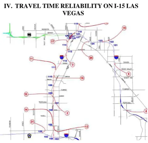
[image:4.595.41.277.355.583.2]

IV. TRAVELTIMERELIABILITYONI-15LAS VEGAS

Figure. 2. DMS on the I-15 corridor in Las Vegas from FAST

In order to demonstrate the proposed reliability measures, travel time data was obtained from The Freeway and Arterial System of Transportation (FAST), an integrated Intelligent Transportation System organization in the Las Vegas area. FAST has approximately 21 Dynamic Message Signs (DMS) mostly distributed along the I-15 as depicted in Fig 2. Travel times are computed through the Incident Processing Module (IPM) in the Freeway Management System (FMS) where it processes detector data from traffic detector stations on the freeways; then, displayed on the DMS (7) (6).

The travel time data obtained spanned a period of eight months, October 2008 through May 2009. Sign identifiers 13 and 17 were selected for analysis since they are located in main thoroughfares that are frequently traversed. Sign identifier 17 is located on the southbound I-15 freeway and it

records the travel time from US-95 to the I-215. Sign identifier 13 is located on the northbound I-15 and it records the travel time from I-215 to US-95. The stretch of freeway covered by the chosen signs witnesses a high percentage of commuters daily which emphasizes the importance of studying it.

A. Data Processing:

Initially, the dynamic message sign data received was a compilation of the date, time, location of the sign identifiers, the end destination, and the time traveled between segments along the I-15. The data record was in comma separated value format where each line of data is text.

Processing of the data was necessary to filter out some of the extraneous information in the data record and also to reorganize the important elements such as the date, time, travel time, the sign identifier, and end destination. For the filtering process and data reorganization, code was written in visual basic for applications (VBA) to automate the process in Excel. The program separated the data into new sheets by the sign identifier and end destination. Within each of these sheets, the data was organized by date and quarter hour. For each quarter hour, the average was computed. Using a pivot table with the day and end destination assigned to the row field, the hour and quarter hour assigned to the column field, and the average travel time assigned to the data field, the data was reorganized into a new table where the averages are computed for each hour while still displaying the quarter hour averages.

By providing estimated travel times with a high degree of reliability, drivers will be able to plan their trips with greater ease and accuracy. After the data is processed, averages are computed for two hour intervals and for days of the week. Averaging the data for every two hour interval allowed for analysis of consistency of travel time between different periods of the day. Averaging the data for days of the week, allows for analysis on a broader scope. Moreover, the consistency of the travel time and the day to day variability can be assessed.

V. RESULTSANDDISCUSSION

Two types of analysis were conducted, day-to-day and within the day reliability, on the DMS data obtained from FAST using the six proposed methods.

A. Classical Methods: Planning Time, Planning Time Index, Buffer Index, Variability Based on Normalized Standard Deviation (NSTD):

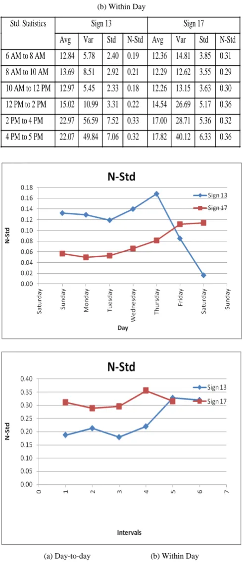
[image:4.595.316.562.663.784.2]

Tables 1(a) and 1(b) list the obtained NSTD for both signs. Fig 3(a) and 3(b) show the normalized standard deviation trends for signs 13 and 17.

Table I Normalized Standard Deviation (a) Day to Day

Std. Statistics Sign 13 Sign 17

Avg Var Std N-Std Avg Var Std N-Std

Monday 13.37 3.12 1.77 0.13 13.86 0.62 0.79 0.06

Tuesday 14.43 3.48 1.87 0.13 13.10 0.42 0.65 0.05

Wednesday 14.97 3.17 1.78 0.12 13.57 0.52 0.72 0.05

Thursday 14.44 4.09 2.02 0.14 12.52 0.69 0.83 0.07

Friday 14.88 6.30 2.51 0.17 14.14 1.32 1.15 0.08

Saturday 11.32 0.92 0.96 0.08 9.67 1.16 1.08 0.11

(5)

(b) Within Day

Std. Statistics Sign 13 Sign 17

Avg Var Std N-Std Avg Var Std N-Std

6 AM to 8 AM 12.84 5.78 2.40 0.19 12.36 14.81 3.85 0.31

8 AM to 10 AM 13.69 8.51 2.92 0.21 12.29 12.62 3.55 0.29

10 AM to 12 PM 12.97 5.45 2.33 0.18 12.26 13.15 3.63 0.30

12 PM to 2 PM 15.02 10.99 3.31 0.22 14.54 26.69 5.17 0.36

2 PM to 4 PM 22.97 56.59 7.52 0.33 17.00 28.71 5.36 0.32

4 PM to 5 PM 22.07 49.84 7.06 0.32 17.82 40.12 6.33 0.36

[image:5.595.35.282.52.624.2]

(a) Day-to-day (b) Within Day

Figure. 3. Normalized Standard Deviation Analysis

The data was processed in two different ways; day to day and within the day. Day to day processing aggregates travel times for a one day at a time which allows comparison of aggregated travel times between different days of the week as well as weekends.

Examining the obtained results for day to day analysis for sign 13 (north bound direction of the I15); higher variability is noted during weekdays. Yet, lower overall NTSD was obtained for sign 17 (I-15 south bound) compared to sign 13. However, results of the processed data during weekends show a higher variability for I-15 south bound (sign 17) than I-15 North bound (sign 13). This

phenomenon may be caused by the fact that drivers’ destination for that section of the freeway is most likely to be in the south direction during weekends since it leads to the center of the city. Overall reliability is not very high which means that traffic conditions on that segment are somewhat inconsistent.

From analyzing the obtained values of the normalized standard deviation for within the day processing, it is noted that the values are higher than the values obtained for day to day analysis. This was expected since traffic conditions vary tremendously throughout the day taking into consideration traffic demand during peak hours as well as off peak hours; however, aggregating the values to represent a day as whole will result in more consistent travel times. Less consistency is noted when travel times are compared for all days as opposed to alike days. This emphasizes the importance of data processing methods and how different processing can give different meanings. Overall, higher reliability is noted on I-15 North which is inconsistent with day to day analysis.

The same data will be analyzed in the following subsections using the various proposed methods in order to extract the information that each one provides.

B. Analysis of Variance ANOVA:

Tables 2(a), 2(b), 2(c), and 2(d) show the F value

obtained from the ANOVA hypothesis test with α = 0.05.

The F values obtained from ANOVA analysis for both signs and the two types of analysis (day to day and within the day) are greater than the critical value Fα which indicates

[image:5.595.353.529.446.707.2]

rejection of the null hypothesis. These results show low consistency in travel times for the studied freeway section reflecting low reliability.

Table II Analysis of Variance (ANOVA)

(a) Sign 13, Day to day

F

P-value

F crit

59.5566

6.94992E-51 2.12399

Sign 13 ANOVA

(b) Sign 17, Day to day

F P-value F crit

253.115 2.6256E-125 2.12399

Sign 17 A NOVA

(c) Sign 13, within the Day

F

P-value

F crit

193.198 1.8349E-151 2.22148

Sign 13 A NOVA

(d) Sign 17, within the day

F P-value F crit

56.4523 7.88115E-53 2.22152

Sign 17 A NOVA

C. Travel Time Mean Estimation:

(6)

is much lower on weekends. Analyzing within the day values, it is noticeable that travel times are much higher in the afternoon than it is in the mornings as shown in Fig 4(a) and 4(b).

Table III Average Travel Time estimation with 95% confidence

(a) Day to Day

Confidence Intervals Sign 13 Sign 17

Times 95th Percentile Times 95th Percentile

Monday 12.95< t < 13.78 16.44 13.67< t < 14.04 15.06

Tuesday 13.99< t < 14.86 17.59 12.95< t < 13.25 14.28

Wednesday 14.55< t < 15.38 17.92 13.40< t < 13.74 14.98

Thursday 13.96< t < 14.90 17.87 12.32< t < 12.71 14.06

Friday 14.29< t < 15.46 18.81 13.87< t < 14.40 16.16

Saturday 11.09< t < 11.54 12.91 9.416< t < 9.916 11.48

Sunday 10.25< t < 10.33 10.62 9.001< t < 9.491 10.76

(b) Within Day

Confidence Intervals Sign 13 Sign 17

Times 95th Percentile Times 95th Percentile

6 AM - 8 AM 12.56< t < 13.11 16.35 12.80< t < 11.91 18.75

8 AM - 10 AM 13.34< t < 14.02 18.82 12.69< t < 11.87 19.59

10 AM - 12 PM 12.69< t < 13.23 17.93 12.67< t < 11.83 18.68

12 PM - 2 PM 14.63< t < 15.40 20.57 15.14< t < 13.94 25.37

2 PM - 4 PM 22.09< t < 23.83 32.84 17.61< t < 16.37 26.92

4 PM - 5 PM 21.25< t < 22.88 32.71 18.55< t < 17.09 30.32

[image:6.595.39.277.140.761.2]

Figure. 4. 95th_{Percentile Travel Times}

D. Reliability as a Measure of Non-failures:

[image:6.595.327.556.229.738.2]

Tables 4(a), 4(b), 4(c), and 4(d) show the results obtained when non-failure analysis is used in determining reliability. Fig 5(b) and 5(a) illustrate the trend for both day to day and within the day. Data was compared to an eleven minute threshold based on a free flow speed of 65 mph as well as segment length which is approximately 10.5 and 7.7 miles for signs 13 and 14, respectively. The results show a higher overall reliability for sign 17 (south bound) than it is for sign 13 (north bound). The studied freeway section is unreliable in the afternoon as well as weekends for both directions. In this case reliability indicates whether travel times are above or below the desired travel time.

Table IV Reliability as a measure of Non-Failure Analysis

(a) Sign 13, Day to Day

Failure Analysis Sign 13

Min Max Range Threshold Success Failure R

Monday 10.58 16.51 5.94 11 3 49 _0.06

Tuesday 10.94 17.68 6.74 1 51 _0.02

Wednesday 11.72 17.99 6.27 0 52 _0.00

Thursday 10.71 17.93 7.22 3 49 _0.06

Friday 10.67 18.85 8.18 3 49 _0.06

Saturday 10.33 12.94 2.61 25 27 _0.48

Sunday 10.07 10.62 0.55 52 0 _1.00

(b) Sign 17, Day to Day

Min Max Range Threshold Success Failure R Monday 11.83 15.10 3.27 11 0 52 _0.00 Tuesday 11.59 14.31 2.72 0 52 _0.00 Wednesday 12.34 15.02 2.67 0 52 _0.00 Thursday 10.73 14.09 3.36 2 50 _0.04 Friday 12.48 16.18 3.71 0 52 _0.00 Saturday 8.26 11.59 3.33 43 9 _0.83 Sunday 8.19 10.77 2.57 52 0 _1.00

(c) Sign 13, Within Day

Min Max Range Threshold Success Failure R 6 AM - 8 AM 9.00 31.10 22.10 11 52 151 0.26 8 AM - 10 AM 9.63 22.94 13.31 48 155 0.24

10 AM - 12 PM 9.63 24.29 14.67 32 171 0.16 12 PM - 2 PM 9.83 30.67 20.83 20 183 0.10 2 PM - 4 PM 9.63 38.85 29.23 14 189 0.07 4 PM - 5 PM 10.17 42.40 32.23 3 200 0.01

(d) Sign 17, Within Day

Min Max Range Threshold Success Failure R

6 AM - 8 AM 7.63 30.98 23.35 11 97 105 0.48

8 AM - 10 AM 7.63 24.73 17.10 94 108 0.47

10 AM - 12 PM 7.63 25.71 18.08 94 108 0.47

12 PM - 2 PM 8.60 33.42 24.81 65 137 0.32

2 PM - 4 PM 8.63 37.23 28.60 21 181 0.10

4 PM - 5 PM 8.08 32.81 24.73 27 175 0.13

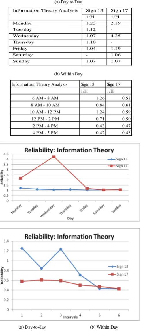
E. Information Theory Based Approach:

(7)

direct indication of reliability with higher values indicating more reliability in the information content.

[image:7.595.39.284.186.764.2]

Conducting the analysis using information theory, results have demonstrated consistency with the values obtained for NSTD showing lower variability thereby higher reliability for sign 17 (south bound) as compared to sign 13 (north bound) during week days. A reversed effect is seen when the analysis is performed within the day.

Table V Information Theory based Reliability

(a) Day to Day

Information Theory Analysis Sign 13 Sign 17

1/H 1/H

Monday 1.23 2.19

Tuesday 1.12 -

Wednesday 1.07 4.25

Thursday 1.10 -

Friday 1.04 1.19

Saturday - 1.06

Sunday 1.07 1.07

(b) Within Day

Information T heory Analysis Sign 13 Sign 17

1/H 1/H

6 AM - 8 AM 1.26 0.58

8 AM - 10 AM 0.84 0.61

10 AM - 12 PM 1.24 0.59

12 PM - 2 PM 0.71 0.50

2 PM - 4 PM 0.43 0.47

4 PM - 5 PM 0.42 0.43

Figure. 5. Information Theory based Reliability

A measure of travel time reliability using information theory can be interpreted as follows. The information contained in the travel time measurements varies both day-today and within the day for both DMS 13 and 17. In comparison, the traditional analysis and failure analysis both indicate that for day-to-day sign 17 is more reliable when compared to sign 13. This conclusion is supported by consistency measurement using the concept of entropy, as demonstrated. For within the day travel time measurements, the information content (H) is higher for 17 indicating that it is less reliable.

VI. CONCLUSION

In this study five reliability approaches were demonstrated, variability based on normalized standard deviation, analysis of Variance (ANOVA), travel time mean estimation, reliability as a measure of non-failures, and information theory based approach. These methods were applied to the I-15 corridor in Las Vegas. Traditional reliability measures were solely based on consistency. However, it does not address the issue of whether the travel time is acceptable or not regardless of its consistency. In other words, consistency of travel times does not necessarily indicate desired travel times. Therefore, reliability measure based on non-failures considers various thresholds when determining reliability. It was also demonstrated that reliability could be obtained based on entropy measure in information theory which analyzes the frequency and therefore the consistency of travel time data.

VII.REFERENCES

[1] Enide A.I. Bogers, Hans WC Van Lint, and HENK J Van Zuylen. Travel Time Reliability: Effective Measures from a Behavioral Point of View. Transportation Research Board, pp 1 - 14, 2008.

[2] Chao Chen, Alexander Skabardonis, and Pravin Varaiya. Travel-Time Reliability as a Measure of Service. Transportation Research Record: Journal of the Transportation Research Board, (1855):74 – 79, 2003.

[3] Jun-Seok Oh and Younshik Chung. Calculation of Travel Time Variability from Loop Detector Data. Transportation Research Record: Journal of the Transportation Research Board, (1945):12 - 23, 2006.

[4] Tilahun, Nebiyou. and Levinson, David. (2010), “A moment of time: Reliability in route choice using stated preference”, Journal of Intelligent Transportation Systems , Vol. 14, pp. 179 –187.

[5] Fosgerau, Mogens. and Karlstrom, Anders. (2010), “The value of reliability”, Transportation Research Part B , Vol. 44, pp. 38–49.

[6] Small, Kenneth A., Winston, Clifford. and Yan, Jia. (2005), “Uncovering the distribution of motorists’ preferences for travel time and reliability”, Econometrica, Vol. 73, pp. 1367–1382.

(8)

[8] Lam S.H., M. Jing, and A.A. Memon. Effects of Real-Time Information on Route Choice Behavior: New Modeling Framework and Simulation Study in Behavioral Responses to ITS. Eindhoven, 2003.

[9] I.G. Black and J.G. Towriss. Demand Effects of Travel Time Reliability. Final report prepared for London assessment division. UK Department of transport, 1993.

[10] J.W.C. Van Lint and H.J. Van Zuylen. Monitoring and Predicting Freeway Travel Time Reliability. Transportation Research Record, (1917):54–62, 2005.

[11] Cambridge Systematics Inc. Traffic Congestion and Reliability Trends and Advanced Strategies for Congestion Mitigation. Prepared for Federal Highway Administration, page 140, 2005.

[12] Mehran, B. and Nakamura, H. 2009. Considering Travel Time Reliability and Safety for Evaluation of Congestion

Relief Schemes on Expressway Segments. IATSS Research, Vol.33, No.1, pp. 55-70

[13] Lomax, T. J. and Schrank, D. L. 2002. Using Travel Time Measure to Estimate Mobility and Reliability in Urban Areas. FHWA Technical Report No. FHWA/TX-02/1511-3

[14] Kimley-Hom and Associates. FreewayManagement System Software Manual. Prepared for Nevada Department of Transportation, (092202006), 2004.

[15] Richard A. Johnson. Miller and Freund’s Probability and Statistics for Engineers. Prentice Hall, 1994.

[16] Gordon Raisbeck. Information Theory. The MIT Press, 1964.

[17] Kimley-Hom and Associates. FreewayManagement System Operator Manual. Prepared for Nevada Department of Transportation, (092202006), 2004.