Timestamped Graphs: Evolutionary Models of Text for Multi Document Summarization

Timestamped Graphs: Evolutionary Models of Text for

Multi-document Summarization

Ziheng Lin, Min-Yen Kan

School of Computing

National University of Singapore

Singapore 177543

{linzihen, kanmy}@comp.nus.edu.sg

Abstract

Current graph-based approaches to auto-matic text summarization, such as Le-xRank and TextRank, assume a static graph which does not model how the in-put texts emerge. A suitable evolutionary text graph model may impart a better un-derstanding of the texts and improve the summarization process. We propose a timestamped graph (TSG) model that is motivated by human writing and reading processes, and show how text units in this model emerge over time. In our model, the graphs used by LexRank and Tex-tRank are specific instances of our time-stamped graph with particular parameter settings. We apply timestamped graphs on the standard DUC multi-document text summarization task and achieve compara-ble results to the state of the art.

1

Introduction

Graph-based ranking algorithms such as Kleinberg’s HITS (Kleinberg, 1999) or Google’s PageRank (Brin and Page, 1998) have been suc-cessfully applied in citation network analysis and ranking of webpages. These algorithms essentially decide the weights of graph nodes based on global topological information. Recently, a number of graph-based approaches have been suggested for NLP applications. Erkan and Radev (2004) intro-duced LexRank for multi-document text summari-zation. Mihalcea and Tarau (2004) introduced TextRank for keyword and sentence extractions. Both LexRank and TextRank assume a fully con-nected, undirected graph, with text units as nodes

and similarity as edges. After graph construction, both algorithms use a random walk on the graph to redistribute the node weights.

Many graph-based algorithms feature an evolu-tionary model, in which the graph changes over timesteps. An example is a citation network whose edges point backward in time: papers (usually) only reference older published works. References in old papers are static and are not updated. Simple models of Web growth are exemples of this: they model the chronological evolution of the Web in which a new webpage must be linked by an incom-ing edge in order to be publicly accessible and may embed links to existing webpages. These models differ in that they allow links in previously gener-ated webpages to be updgener-ated or rewired. However, existing graph models for summarization – LexRank and TextRank – assume a static graph, and do not model how the input texts evolve. The central hypothesis of this paper is that modeling the evolution of input texts may improve the sub-sequent summarization process. Such a model may be based on human writing/reading process and should show how just composed/consumed units of text relate to previous ones. By applying this model over a series of timesteps, we obtain a rep-resentation of how information flows in the con-struction of the document set and leverage this to construct automatic summaries.

and apply it to the standard Document Understand-ing Conference (DUC) datasets. We discuss the resulting performance in Section 5.

2

Timestamped Graph

We believe that a proper evolutionary graph model of text should capture the writing and reading processes of humans. Although such human proc-esses vary widely, when we limit ourselves to ex-pository text, we find that both skilled writers and readers often follow conventional rhetorical styles (Endres-Niggemeyer, 1998; Liddy, 1991). In this work, we explore how a simple model of evolution affects graph construction and subsequent summa-rization. In this paper, our work is only exploratory and not meant to realistically model human proc-esses and we believe that deep understanding and inference of rhetorical styles (Mann and Thompson, 1988) will improve the fidelity of our model. Nev-ertheless, a simple model is a good starting point.

We make two simple assumptions:

1: Writers write articles from the first sentence to the last;

2: Readers read articles from the first sentence to the last.

The assumptions suggest that we add sentences into the graph in chronological order: we add the first sentence, followed by the second sentence, and so forth, until the last sentence is added.

These assumptions are suitable in modeling the growth of individual documents. However when dealing with multi-document input (common in DUC), our assumptions do not lead to a straight-forward model as to which sentences should ap-pear in the graph before others. One simple way is to treat document problems simply as multi-ple instances of the single document problem, which evolve in parallel. Thus, in multi-document graphs, we add a sentence from each document in the input set into the graph at each timestep. Our model introduces a skew variable to model this and other possible variations, which is detailed later.

The pseudocode in Figure 1 summarizes how we build a timestamped graph for multi-document input set. Informally, we build the graph itera-tively, introducing new sentence(s) as node(s) in

the graph at each timestep. Next, all sentences in the graph pick other previously unconnected ones to draw a directed edge to. This process continues until all sentences are placed into the graph.

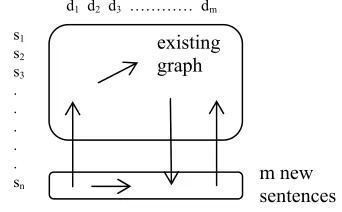
Figure 2 shows this graph building process in mid-growth, where documents are arranged in col-umns, with dx represents the xth document and sy

represents the yth _{sentence of each document. The}

bottom shows the nth _{sentences of all m documents}

being added simultaneously to the graph. Each new node can either connect to a node in the existing graph or one of the other m-1 new nodes. Each existing node can connect to another existing node or to one of the m newly-introduced nodes. Note that this model differs from the citation networks in such that new outgoing edges are introduced to old nodes, and differs from previous models for Web growth as it does not require new nodes to have incoming edges.

Figure 2: Snapshot of a timestamped graph.

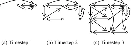
Figure 3 shows an example of the graph building process over three timesteps, starting from an empty graph. Assume that we have three docu-ments and each document has three sentences. Let dxsy indicate the yth sentence in the xth document.

At timestep 1, sentences d1s1, d2s1 and d3s1 are s1

s2 s3 . . . . . sn

d1 d2 d3 ………… dm

existing graph

Figure 1: Pseudocode for a specific instance of a

timestamped graph algorithm Input: M, a cluster of m documents relating to a

common event;

Let: i = index to sentences, initially 1;

G = the timestamped graph, initially empty. Step 1: Add the ith sentence of all documents into G.

Step 2: Let each existing sentence in G choose and

connect to one other existing sentence in G.

The chosen sentence must be sentence which has not been previously chosen by this sentence in previous iterations.

Step 3: if there are no new sentences to add, break; else i++, goto Step 1.

Output: G, a timestamped graph.

added to the graph. Three edges are introduced to the graph, in which the edges are chosen by some strategy; perhaps by choosing the candidate sen-tence by its maximum cosine similarity with the sentence under consideration. Let us say that this process connects d1s1→d3s1, d2s1→d3s1 and

d3s1→d2s1. At timestep 2, sentences d1s2, d2s2 and

d3s2 are added to the graph and six new edges are

introduced to the graph. At timestep 3, sentences d1s3, d2s3 and d3s3 are added to the graph, and nine

new edges are introduced.

(a) Timestep 1 (b) Timestep 2 (c) Timestep 3

Figure 3: An example of the growth of a

timestamped graph.

The above illustration is just one instance of a timestamped graph with specific parameter settings. We generalize and formalize the timestamped graph algorithm as follows:

Definition: A timestamped graph algorithm tsg(M) is a 9-tuple (d, e, u, f, σ, t, i, s, τ) that speci-fies a resulting algorithm that takes as input the set of texts M and outputs a graph G, where:

d specifies the direction of the edges, d∈{f, b, u}; e is the number of edges to add for each vertex

in G at each timestep, e∈ℤ +;

u is 0 or 1, where 0 and 1 specifies unweighted and weighted edges, respectively;

f is the inter-document factor, 0 ≤f≤ 1;

σ is a vertex selection function σ(u, G) that takes in a vertex u and G, and chooses a vertex v∈G; t is the type of text units, t∈{word, phrase,

sentence, paragraph, document}; i is the node increment factor, i∈ℤ +_;

s is the skew degree, s ≥ -1 and s∈ℤ , where -1 represent free skew and 0 no skew;

τ is a document segmentation function τ(•).

In the TSG model, the first set of parameters d, e, u, f deal with the properties of edges; σ, t, i, s deal with properties of nodes; finally, τ is a

func-tion that modifies input texts. We now discuss the first eight parameters; the relevance of τ will be expanded upon later in the paper.

2.1

We can specify the direction of information flow by setting different d values. When a node v1

chooses another node v2 to connect to, we set d to f

to represent a forward (outgoing) edge. We say that v1 propagates some of its information into v2.

When letting a node v1 choose another node v2 to

connect to v1 itself, we set d to b to represent a

backward (incoming) edge, and we say that v1

re-ceives some information from v2. Similarly, d = u

specifies undirected edges in which information propagates in both directions. The larger amount of information a node receives from other nodes, the higher the importance of this node.

Our toy example in Figure 3 has small dimen-sions: three sentences for each of three documents. Experimental document clusters often have much larger dimensions. In DUC, clusters routinely con-tain over 25 documents, and the average length for documents can be as large as 50 sentences. In such cases, if we introduce one edge for each node at each timestep, the resulting graph is loosely con-nected. We let e be the number of outgoing edges for each sentence in the graph at each timestep. To introduce more edges into the graph, we increase e. We can also incorporate unweighted or weighted edges into the graph by specifying the value of u. Unweighted edges are good when rank-ing algorithms based on in-degree of nodes are used. However, unlike links between webpages, edges between text units often have weights to in-dicate connection strength. In these cases, un-weighted edges lose information and a un-weighted representation may be better, such as in cases where PageRank-like algorithms are used for rank-ing.

Edges can represent information flow from one node to another. We may prefer intra-document edges over inter-document edges, to model the in-tuition that information flows within the same document more likely than across documents. Thus we introduce an inter-document factor f, where 0 ≤

2.2

In Figure 1 Step 2, every existing node has a chance to choose another existing node to connect to. Which node to choose is decided by the selec-tion strategy σ. One strategy is to choose the node with the highest similarity. There are many similar-ity functions to use, including token-based Jaccard similarity, cosine similarity, or more complex models such as concept links (Ye et al., 2005).

t controls the type of text unit that represents nodes. Depending on the application, text units can be words, phrases, sentences, paragraphs or even documents. In the task of automatic text summari-zation, systems are conveniently assessed by let-ting text units be sentences.

i controls the number of sentences entering the graph at every iteration. Certain models, such as LexRank, introduce all of the input sentences in one time step (i.e., i = Lmax, where Lmax is the

maximum length of the input documents), com-pleting the construction of G in one step. However, to model time evolution, i needs to be set to a value smaller than this.

Most relevant to our study is the skew parame-ter s. Up to now, the TSG models discussed all assume that authors start writing all documents in the input set at the same time. It is reflected by adding the first sentences of all documents simul-taneously. However in reality, some documents are authored later than others, giving updates or report-ing changes to events reported earlier. In DUC document clusters, news articles are typically taken from two or three different newswire sources. They report on a common event and thus follow a story-line. A news article usually gives summary about what have been reported in early articles, and gives updates or changes on the same event.

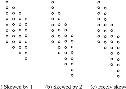
To model this, we arrange the documents in ac-cordance with the publishing time of the docu-ments. The earliest document is assigned to column 1, the second earliest document to column 2, and so forth, until the latest document is as-signed to the last column. The graph construction process is the same as before, except that we delay adding the first sentences of later documents until a proper iteration, governed by s. With s = 1, we de-lay the addition of the first sentence of column 2 until the second timestep, and delay the addition of the first sentence of column 3 until the third timestep. The resulting timestamped graph is

skewed by 1 timestep (Figure 4 (a)). We can in-crease the skew degree s if the time intervals be-tween publishing time of documents are large. Figure 4 (b) shows a timestamped graph skewed by 2 timesteps. We can also skew a graph freely by setting s to -1. When we start to add the first sen-tence dis1 of a document di, we check whether there

are existing sentences in the graph that want to connect to dis1 (i.e., that σ (•,G) = dis1). If there is,

we add dis1 to the graph; else we delay the addition

and reassess again in next timestep. The result is a freely skewed graph (Figure 4 (c)). In Figure 4 (c), we start adding the first sentences of documents d2

to d4 at timesteps 2, 5 and 7, respectively. At

timestep 1, d1s1 is added into the graph. At

timestep 2, an existing node (d1s1 in this case)

wants to connect to d2s1, so d2s1 is added. d3s1 is

added at timestep 5 as no existing node wants to connect to d3s1 until timestep 5. Similarly, d4s1 is

added until some nodes choose to connect to it at timestep 7. Notice that we hide edges in Figure 4 for clarity.

(a) Skewed by 1 (b) Skewed by 2 (c) Freely skewed

Figure 4: Skewing the graphs. Edges are hidden for clarity. For each graph, the leftmost column is the earliest document.

Documents are then chronologically ordered, with the right-most one being the latest.

3

Comparison and Properties of TSG

The TSG representation generalizes many pos-sible specific algorithm configurations. As such, it is natural that previous works can be cast as spe-cific instances of a TSG. For example, we can suc-cinctly represent the algorithm used in the running example in Section 2 as the tuple (f, 1, 0, 1, max-cosine-based, sentence, 1, 0, null). LexRank and TextRank can also be cast as TSGs: (u, N, 1, 1, cosine-based, sentence, Lmax, 0, null) and (u, L, 1, 1,

null). As LexRank is applied in multi-document summarizations, e is set to the total number of sen-tences in the cluster, N, and i is set to the maxi-mum document length in the cluster, Lmax.

TextRank is applied in single-document summari-zation, so both its e and i are set to the length of the input document, L. This compact notation empha-sizes the salient differences between these two al-gorithm variants: namely that, e, σand i.

Despite all of these possible variations, all timestamped graphs have two important features, regardless of their specific parameter settings. First, nodes that were added early have more chosen edges than nodes added later, as visible in Figure 3 (c). If forward edges (d = f) represent information flow from one node to another, we can say that more information is flowing from these early nodes to the rest of the graph. The intuition for this is that, during the writing process of articles, early sentences have a greater influence to the develop-ment of the articles’ ideas; similarly, during the reading process, sentences that appear early con-tribute more to the understanding of the articles.

The fact that early nodes stay in the graph for a longer time leads to the second feature: early nodes may attract more edges from other nodes, as they have larger chance to be chosen and connected by other nodes. This is also intuitive for forward edges (d = f): during the writing process, later sen-tences refer back to early sensen-tences more often than vice versa; and during the reading process, readers tend to re-read early sentences when they are not able to understand the current sentence.

4

Random Walk

Once a timestamped graph is built, we want to compute an importance score for each node. These scores are then used to determine which nodes (sentences) are the most important to extract sum-maries from. The graph G shows how information flows from node to node, but we have yet to let the information actually flow. One method to do this is to use the in-degree of each node as the score. However, most graph algorithms now use an itera-tive method that allows the weights of the nodes redistribute until stability is reached. One method for this is by applying a random walk, used in Pag-eRank (Brin and Page, 1998). In PagPag-eRank the Web is treated as a graph of webpages connected by links. It assumes users start from a random

webpage, moving from page to page by following the links. Each user follows the links at random until he gets “bored” and jumps to a random web-page. The probability of a user visiting a webpage is then proportional to its PageRank score. PageR-ank can be iteratively computed by:

∑

PR α α (1)

where N is the total number of nodes in the graph, In(u) is the set of nodes that point to u, and Out(u) is the set of nodes that node u points to. α is a damping factor that can be set between 0 and 1, which has the role of integrating into the model the probability of jumping from a given node to an-other random node in the graph. In the context of web surfing, a user either clicks on a link on the current page at random with probability 1 - α, or opens a completely new random page with prob-ability α.

Equation 1 does not take into consideration the weights of edges, as the original PageRank defini-tion assumes hyperlinks are unweighted. Thus we can use Equation 1 to rank nodes for an un-weighted timestamped graph. To integrate edge weights into the graph, we modify Eq. 1, yielding:

∑ ∑

vu _{PR v}

w w N

u

PR α α (2)

where Wvu represents the weight of the edge

point-ing from v to u.

As we may have a query for each document cluster, we also wish to take queries into consid-eration in ranking the nodes. Haveliwala (2003) introduces a topic-sensitive PageRank computation. Equations 1 and 2 assume a random walker jumps from the current node to a random node with prob-ability α. The key to creating topic-sensitive Pag-eRank is that we can bias the computation by restricting the user to jump only to a random node which has non-zero similarity with the query. Ot-terbacher et al. (2005) gives an equation for topic-sensitive and weighted PageRank as:

∑ ∑

∑

where S is the set of all nodes in the graph, and sim(u, Q) is the similarity score between node u and the query Q.

5

Experiments and Results

We have generalized and formalized evolutionary timestamped graph model. We want to apply it on automatic text summarization to confirm that these evolutionary models help in extracting important sentences. However, the parameter space is too large to test all possible TSG algorithms. We con-duct experiments to focus on the following re-search questions that relating to 3 TSG parameters - e, u and s, and the topic-sensitivity of PageRank.

Q1: Do different e values affect the summariza-tion process?

Q2: How do topic-sensitivity and edge weight-ing perform in runnweight-ing PageRank?

Q3: How does skewing the graph affect infor-mation flow in the graph?

The datasets we use are DUC 2005 and 2006. These datasets both consist of 50 document clus-ters. Each cluster consists of 25 news articles which are taken from two or three different news-wire sources and are relating to a common event, and a query which contains a topic for the cluster and a sequence of statements or questions. The first three experiments are run on DUC 2006, and the last experiment is run on DUC 2005.

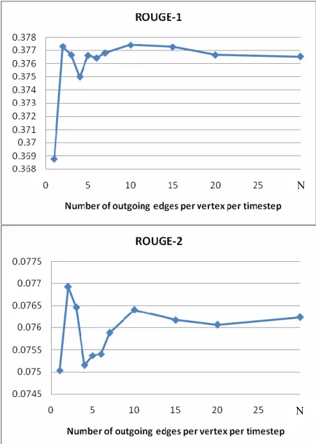
In the first experiment, we analyze how e, the number of chosen edges for each node at each timestep, affects the performance, with other pa-rameters fixed. Specifically the TSG algorithm we use is the tuple (f, e, 1, 1, max-cosine-based, sen-tence, 1, 0, null), where e is being tested for differ-ent values. The node selection function max-cosine-based takes in a sentence s and the current graph G, computes the TFIDF-based cosine simi-larities between s and other sentences in G, and connects s to e sentence(s) that has(have) the high-est cosine score(s) and is(are) not yet chosen by s in previous iterations. We run topic-sensitive Pag-eRank with damping factor α set to 0.5 on the graphs. Figures 5 (a)-(b) shows the ROUGE-1 and ROUGE-2 scores with e set to 1, 2, 3, 4, 5, 6, 7, 10, 15, 20 and N, where N is the total number of sen-tences in the cluster. We succinctly represent

LexRank graphs by the tuple (u, N, 1, 1, cosine-based, sentence, Lmax, 0, null) in Section 3; it can

also be represented by a slightly different tuple (f, N, 1, 1, max-cosine-based, sentence, 1, 0, null). It differs from the first representation in that we itera-tively add 1 sentence for each document in each timestep and let all nodes in the current graph con-nect to every other node in the graph. In this ex-periment, when e is set to N, the timestamped graph is equivalent to a LexRank graph. We do not use any reranker in this experiment.

N

N

Figure 5: (a) ROUGE-1 and (b) ROUGE-2 scores for

timestamped graphs with different e settings. N is the total number of sentences in the cluster.

greater than 10. The reason for this is that the higher values of e make the graph converge to a fully connected graph so that the performance starts to converge and display less variability.

We run a second experiment to analyze how topic-sensitivity and edge weighting affect the sys-tem performance. We use concept links (Ye et al., 2005) as the similarity function and a MMR reranker to remove redundancy. Table 1 shows the results. We observe that both topic-sensitive Pag-eRank and weighted edges perform better than ge-neric PageRank on unweighted timestamped graphs. When topic-sensitivity and edge weighting are both set to true, the system gives the best per-formance.

Topic-sensitive

Weighted edges

ROUGE-1 ROUGE-2

No No 0.39358 0.07690

Yes No 0.39443 0.07838

No Yes 0.39823 0.08072

Yes Yes 0.39845 0.08282

Table 1: ROUGE-1 and ROUGE-2 scores for different

com-binations of topic-sensitivity and edge weighting(u) settings.

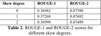
To evaluate how skew degree s affects summa-rization performance, we use the parameter setting from the first experiment, with e fixed to 1. Spe-cifically, we use the tuple (f, 1, 1, 1, concept-link-based, sentence, 1, s, null), with s set to 0, 1 and 2. Table 2 gives the evaluation results. We observe that s = 1 gives the best ROUGE-1 and ROUGE-2 scores. Compared to the system without skewing (s = 0), s = 2 gives slightly better ROUGE-1 score but worse ROUGE-2 score. The reason for this is that s = 2 introduces a delay interval that is too large. We expect that a freely skewed graph (s = -1) will give more reasonable delay intervals.

Skew degree ROUGE-1 ROUGE-2

0 0.36982 0.07580 1 0.37268 0.07682 2 0.36998 0.07489

Table 2: ROUGE-1 and ROUGE-2 scores for

different skew degrees.

We tune the system using different combina-tions of parameters, and the TSG algorithm with tuple (f, 1, 1, 1, concept-link-based, sentence, 1, 0, null) gives the best scores. We run this TSG algo-rithm with topic-sensitive PageRank and MMR reranker on DUC 2005 dataset. The results show

that our system ranks third in both ROUGE-2 and ROUGE-SU4 scores.

Rank System ROUGE-2 System ROUGE-SU4

1 15 0.0725 15 0.1316

2 17 0.0717 17 0.1297

3 TSG 0.0712 TSG 0.1285

4 10 0.0698 8 0.1279

5 8 0.0696 4 0.1277

Table 3: top ROUGE-2 and ROUGE-SU4

scores in DUC 2005. TSG is our system.

6

Discussion

A closer inspection of the experimental clusters reveals one problem. Clusters that consist of documents that are of similar lengths tend to per-form better than those that contain extremely long documents. The reason is that a very long docu-ment introduces too many edges into the graph. Ideally we want to have documents with similar lengths in a cluster. One solution to this is that we split long documents into shorter documents with appropriate lengths. We introduce the last parame-ter in the formal definition of timestamped graphs, τ, which is a document segmentation function τ(•). τ(M) takes in as input a set of documents M, ap-plies segmentation on long documents to split them into shorter documents, and output a set of docu-ments with similar lengths, M’. Slightly better re-sults are achieved when a segmentation function is applied. One shortcoming of applying τ(•) is that when a document is split into two shorter ones, the early sentences of the second half now come be-fore the later sentences of the first half, and this may introduce inconsistencies in our representation: early sentences of the second half contribute more into later sentences of the first half than the vice versa.

7

Related Works

Dorogovtsev and Mendes (2001) suggest schemes of the growth of citation networks and the Web, which are similar to the construction process of timestamped graphs.

similarity graphs. Degree centrality is defined as the in-degree of vertices after removing edges which have cosine similarity below a pre-defined threshold. LexRank with threshold is the second method that applies random walk on an un-weighted similarity graph after removing edges below a pre-defined threshold. Continuous Le-xRank is the last method that applies random walk on a fully connected, weighted similarity graph. LexRank has been applied on multi-document text summarization task in DUC 2004, and topic-sensitive LexRank has been applied on the same task in DUC 2006.

Mihalcea and Tarau (2004) independently pro-posed another similar graph-based random walk model, TextRank. TextRank is applied on keyword extraction and single-document summarization. Mihalcea, Tarau and Figa (2004) later applied Pag-eRank to word sense disambiguation.

8

Conclusion

We have proposed a timestamped graph model which is motivated by human writing and reading processes. We believe that a suitable evolutionary text graph which changes over timesteps captures how information propagates in the text graph. Ex-perimental results on the multi-document text summarization task of DUC 2006 showed that when e is set to 2 with other parameters fixed, or when s is set to 1 with other parameters fixed, the graph gives the best performance. It also showed that topic-sensitive PageRank and weighted edges improve summarization process. This work also unifies representations of graph-based summariza-tion, including LexRank and TextRank, modeling these prior works as specific instances of time-stamped graphs.

We are currently looking further on skewed timestamped graphs. Particularly we want to look at how a freely skewed graph propagates informa-tion. We are also analyzing in-degree distribution of timestamped graphs.

Acknowledgments

The authors would like to thank Prof. Wee Sun Lee for his very helpful comments on random walk and the construction process of timestamped graphs, and thank Xinyi Yin (Yin, 2007) for his help in spearheading the development of this work. We also would like to thank the reviewers for their

helpful suggestions in directing the future of this work.

References

Jon M. Kleinberg. 1999. Authoritative sources in a hy-perlinked environment. In Proceedings of ACM-SIAM Symposium on Discrete Algorithms, 1999. Sergey Brin and Lawrence Page. 1998. The anatomy of

a large-scale hypertextual Web search engine. Com-puter Networks and ISDN Systems, 30(1-7).

Günes Erkan and Dragomir R. Radev. 2004. LexRank: Graph-based centrality as salience in text summari-zation. Journal of Artificial Intelligence Research, (22).

Rada Mihalcea and Paul Tarau. 2004. TextRank: Bring-ing order into texts. In Proceedings of EMNLP 2004. Rada Mihalcea, Paul Tarau, and Elizabeth Figa. 2004.

PageRank on semantic networks, with application to word sense disambiguation. In Proceedings of COLING 2004.

S.N. Dorogovtsev and J.F.F. Mendes. 2001. Evolution of networks. Submitted to Advances in Physics on 6th March 2001.

Shiren Ye, Long Qiu, Tat-Seng Chua, and Min-Yen Kan. 2005. NUS at DUC 2005: Understanding docu-ments via concepts links. In Proceedings of DUC 2005.

Xinyi Yin, 2007. Random walk and web information processing for mobile devices. PhD Thesis.

Taher H. Haveliwala. 2003. Topic-sensitive pagerank: A context-sensitive ranking algorithm for web search. IEEE Transactions on Knowledge and Data Engi-neering

Jahna Otterbacher, Günes Erkan and Dragomir R. Radev. 2005. Using Random Walks for Question-focused Sentence Retrieval. In Proceedings of HLT/EMNLP 2005.

Brigitte Endres-Niggemeyer. 1998. Summarizing infor-mation. Springer New York.

Elizabeth D. Liddy. 1991. The discourse-level structure of empirical abstracts: an exploratory study. Infor-mation Processing and Management 27(1):55-81. William C. Mann and Sandra A. Thompson. 1988.