An Approximate Microaggregation Approach for
Microdata Protection
Xiaoxun Sun
1,
Hua Wang
1,
Jiuyong Li
2Yanchun Zhang
3 1Department of Mathematics & ComputingUniversity of Southern Queensland, Australia 2School of Computer and Information Science
University of South Australia, Australia 3School of Engineering and Science
Victoria University, Australia
Abstract
Microdata protection is a hot topic in the field of Statistical Disclosure Control, which
has gained special interest after the disclosure of 658000 queries by the America Online
(AOL) search engine in August 2006. Many algorithms, methods and properties have
been proposed to deal with microdata disclosure. One of the emerging concepts in
mi-crodata protection is k-anonymity, introduced by Samarati and Sweeney. k-anonymity
provides a simple and efficient approach to protect private individual information and is
gaining increasing popularity. k-anonymity requires that every record in the microdata
table released be indistinguishably related to no fewer than krespondents.
In this paper, we apply the concept of entropy to propose a distance metric to
eval-uate the amount of mutual information among records in microdata, and propose a
method of constructing dependency tree to find the key attributes, which we then use
to process approximate microaggregation. Further, we adopt this new microaggregation
technique to study k-anonymity problem, and an efficient algorithm is developed.
Ex-perimental results show that the proposed microaggregation technique is efficient and
1
Introduction
British politicians gasped with astonishment when they were told on November 20th, 2007,
that two computer disks full of personal data of 25m British individuals had gone missing
[24]. The fate of the disks is unknown and the privacy of the individuals, whose personal data
are lost, is in danger. Unfortunately, this is the latest in a series of similar incidences. In October, HM’s Revenue and Customs (HMRC) lost another disk containing pension records
of 15,000 people, and it also lost a laptop containing personal data on 400 people in September
[7]. Data on 26.5m people were stolen from the home of an employee of the Department of
Veterans Affairs in America in 2006, and 658000 queries were disclosed by the AOL search
engine in August of the same year [15]. These pitfalls are not new. Due to the great advances
in the information and communication technologies, it is very easy to gather large amounts
of personal data, and mistakes such as those described are magnified.
There are many real-life situations in which personal data is stored: For example: (i)
Electronic commerce results in the automated collection of large amounts of consumer data. These data, which are gathered by many companies, are shared with subsidiaries and partners.
(ii) Health care is a very sensitive sector with strict regulations. In the U.S., the Privacy
Rule of the Health Insurance Portability and Accountability Act (HIPAA [16]) requires the
strict regulation of protected health information for use in medical research. In most western
countries, the situation is similar, (see e.g. [2]). (iii) Cell phones have become ubiquitous
and services related to the current position of the user are growing fast. If the queries that a
user submits to a location-based server are not securely managed, it could be possible to infer
the consumer habits of the user [33]. (iv) The massive deployment of the Radio Frequency
IDentification (RFID) technology is a reality. On the one hand, this technology will increase the efficiency of supply chains and will eventually replace bar codes. On the other hand, the
existence of RFID tags in almost every object could be seen as a privacy problem [34].
In addition to these real-life situations, most countries have legislation which compels
national statistical agencies to guarantee statistical confidentiality when they release data
collected from citizens or companies; see [23] for regulations in the European Union, [26] for
regulations in Canada, [27] for regulations in the U.S, and [28] for regulations in Australia.
agencies, Internet companies, manufacturers, etc; and many efforts have been devoted to
develop techniques guaranteeing some degree of personal privacy.
In order to protect privacy, Samarati and Sweeney [31, 38, 29, 30] proposed the k
-anonymity model, where some of the quasi-identifier fields are suppressed or generalized so
that, for each record in the modified table, there are at least k−1 other records in the
mod-ified table that are identical to it with respect to the quasi-identifier attributes. The general
approach adopted in the literatures to achieve k-anonymity is suppression/generalization, so
that minimizing information loss translates to reducing the number and/or the magnitude of
suppressions and generalizations [1, 29, 38, 35, 37, 39, 20, 19, 21].
Another method to achieve anonymity is through microaggregation [12, 11, 32].
Microag-gregation is a Statistical Disclosure Control (SDC) technique consisting in the agMicroag-gregation of
individual data. It can be considered as an SDC sub-discipline devoted to the protection of
microdata. Microaggregation can be seen as a clustering problem with constraints on the size
of the clusters. It is somehow related to other clustering problems (e.g., dimension reduction
or minimum squares design of clusters). However, unlike clustering, microaggregation is not
considered with the number of clusters or the number of dimensions, but only the minimum number of elements that are grouped in each cluster.
1.1
Motivation
As stated in [9, 10, 11], the result and execution time of miroaggregation depends on the
number of the variables used in the microaggregation process. Microaggregation using fewer
variables sometimes offer the best solution. The question of interest is: Do we have to use
all the dimension resources (attributes) in the microaggregation, or can we use only a small
number of the attributes in the microaggregation process and obtain better solutions?
This paper is highly motivated by this. To answer the question, we introduce the concept of
entropy, an important concept in information theory, and propose a distance metric to evaluate
the amount of the mutual information among records in the microdata, and propose the
method of constructing dependency tree to find the key attributes, which we can use to process approximate microaggregation. Further, we apply this new microaggregation technique to
results show that the proposed microaggregation technique is efficient and effective in terms
of running time and information loss.
Our Contributions:
•We propose a novel metric to measure the mutual information between attributes in the
microdata based on the concept of entropy, which captures the expected uncertainty in the
attribute pairs and the mutual information between them. We also discuss the properties of this metric.
• Based on this mutual information measure, we develop a simple, yet efficient algorithm
to find the best dependency tree from the given microdata, and we also discuss how to
select key attributes from the best dependency tree, and how to use it for the approximate
microaggregation.
•We apply our technique to k-anonymity problem, and develop an efficient algorithm for
it. Experimental results show that the proposed microaggregation technique is effective and
efficient compared with the previous microaggregation method.
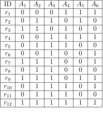
Running Example
ID A1 A2 A3 A4 A5 A6
r1 0 0 0 1 1 1
r2 0 1 1 0 1 0
r3 1 1 0 1 0 0
r4 0 0 1 1 1 1
r5 0 1 1 1 0 0
r6 0 0 1 0 0 1
r7 1 1 1 0 0 1
r8 0 1 1 0 0 0
r9 1 1 1 0 1 1
r10 0 1 1 1 0 1
r11 0 1 1 1 0 0
r12 1 1 1 1 1 1
For the simplicity of illustration, we use the data shown in Table 1 as our running example.
There are 12 records{r1, r2,· · · , r12}in the sample data and each record contains 6 attributes
{A1,· · · , A6}. For each attribute Ai (1 ≤ i ≤ 6), we define the probability P(Ai = x) as
the fraction of rows whose projection onto Ai is equal to x, where x ∈ {0,1}. For instance,
P(A1 = 1) = 1/3,P(A3 = 0) = 1/6 andP(A1 = 1, A3 = 0) = 1/12.
2
Background
Many techniques have been proposed to deal with the anonymity problem. In this section,
we introduce some basic concepts regarding this. First, we take a look at some fundamental
concepts of microaggregation and k-anonymity. Then, we show how to achieve k-anonymity
through microaggregation.
2.1
Microaggregation
Statistical Disclosure Control (SDC) seeks to transform data in such a way that the data can
be publicly released whilst preserving utility and privacy, where the latter means avoiding
disclosure of information that can be linked to specific individual or corporate respondent
entities. Microaggregation is an SDC technique consisting in the aggregation of individual data. It can be considered as an SDC sub-discipline devoted to the protection of the
micro-data. Microaggregation can be seen as a clustering problem with constraints on the size of
the clusters. It is somehow related to other clustering problems (e.g., dimension reduction or
minimum squares design of clusters). However, the main difference of the microaggregation
problem is that it does not consider the number of clusters to generate or the number of
dimensions to reduce, but only the minimum number of elements that are grouped in the
same cluster.
Microaggregation has been used for several years in different countries. It started at
Eurostat [8] in the early nineties, and has since then been used in Germany [25] and several other countries [13]. Microaggregation is relevant not only with SDC, but also in artificial
intelligence [10]. In the latter field, the application is to increase the knowledge of a system
Gender Age Postcode Problem male middle 4350 stress male middle 4350 obesity male young 4351 stress female young 4352 obesity
female old 4353 stress female old 4353 obesity
Table 2: A raw microdata
Gender Age Postcode Problem male middle 4350 stress male middle 4350 obesity
∗ young 435∗ stress
∗ young 435∗ obesity female old 4353 stress female old 4353 obesity
Table 3: A 2-anonymous microdata
6 9 5 10 11 4
5 10 5 10 5 10
Average Origianl data
Microaggregated data record
Figure 1: Example of microaggregation
used in data mining in order to scale down or even compress the data set while minimizing
the information loss.
When we microaggregate data we have to keep two goals in mind: (i) Preserving data
utility. To do this, we should introduce as little noise as possible into the data; i.e., we should
aggregate similar elements instead of different ones. In the example in Figure 1, groups of
three elements are built and aggregated. Note that elements in the same aggregation group
are similar. (ii)Protecting the privacy of the individuals. Data have to be sufficiently modified
to make re-identification difficult; i.e., by increasing the number of aggregated elements, we increase data privacy. In the example in Figure 1, after aggregating the chosen elements, it is
impossible to distinguish them, so that the probability of linking any individual is inversely
proportional to the number of aggregated elements.
In order to determine whether two elements are similar, a similarity function such as
measure is the Sum of Squared Errors (SSE). The SSE is the sum of squared distances from
the centroid of each group to every record in the group, and is defined as:
SSE =
s
∑
i=1
ni
∑
j=1
(xij −x¯i)′(xij −x¯i) (1)
where s is the number of groups, ni is the number of records in the ith group, xij is the jth
record in the ith group and ¯x
i is the average record of the ith group. Optimal multivariate
microaggregation, that is, with minimum SSE, was shown to be NP-hard in [22]. The only
practical microaggregation methods are heuristic.
2.2
K
-Anonymity
k-anonymity, suggested by Samarati and Sweeney [31, 38, 29, 30], is an interesting approach to
reduce the conflict between information loss and privacy protection. To define ofk-anonymity,
we need to enumerate the various types of attributes that can appear in a microdata set T:
• Identifier attributes that can be used to identify a record, such as Name and Medicare
card. Since our objective is to prevent sensitive information from being linked to specific
respondents, we will assume in what follows thatidentifier attributes in the microdata have
been removed or encrypted in a pre-processing step.
• Quasi-identifier (QI) attributes are those, such as Postcode and Age, that in combination,
can be linked with external information to re-identify (some of) the respondents to whom
(some of) the records in the microdata belong. Unlike identifier attributes, QI attributes
can not be removed from the microdata, because any attribute is potentially aQI attribute.
• Sensitive attributes that are assumed to be unknown to an intruder and need to be
pro-tected, such as Disease or ICD-9 Code1.
Definition 1 (k-anonymity). A protected microdata set is said to satisfy k-anonymity, if,
for each combination of QI attributes, at least k records exist in the microdata sharing that
combination
Note that, if a protected microdata T′ satisfies k-anonymity, an intruder trying to link
T′ with an external non-anonymous data source will find at least k records in T′ that match
any value of the QI attributes the intruder use for linkage. Thus re-identification, i.e.,
map-ping a record in T′ to a non-anonymous record in the external data source, is not possible.
For example, Table 3 is a 2 anonymous view of Table 2 if QI attributes are {Gender, Age,
Postcode}.
If for a givenk,k-anonymity is assumed to be enough protection for respondents, one can
concentrate on minimizing information loss with the only constraint thatk-anonymity should
be satisfied. This is a clean way of solving the tension between data protection and data
utility. The general approach adopted in the literature to achieve k-anonymity is
suppres-sion/generalization, so that minimizing information loss translates to reducing the number
and/or the magnitude of suppressions and generalizations [29, 38, 35]. Generalization consists
in substituting the values of a given attribute with more general values. We use ∗ to denote
the more general value. For instance, in Table 3, Postcode 4351 and 4352 are generalized to
435∗. Suppression refers to removing the part or entire value of attributes from the microdata.
Note that suppressing an attribute to reach k-anonymity can equivalently be modeled via a
generalization of all the attribute values to ∗.
The drawbacks of partially suppressed and coarsened data for analysis were highlighted
in [12]:
1. Satisfying k-anonymity with minimum data modification using generalization
(recod-ing) and local suppression was shown to be NP-hard by Meyerson and Williams [21], Aggarwal et al. [1] and Sun et al. [36];
2. Using global recoding for generalization causes too much information loss, and using
local recoding complicates data analysis by causing old and new categories to co-exist
3. There is no standard way of using local suppression and analyzing partially suppressed
data usually requires specific software;
4. Last but not least, when numerical attributes are generalized, they become non-numerical.
Joint multivariate microaggregation of all QI attributes with minimum group size k was
proposed in [12] as an alternative to achievek-anonymity. Besides being simpler, this
alterna-tive has the advantage of yielding complete data without any coarsening (nor categorization
in the case of numerical data). Other proposals [18, 35, 36, 37] generalize ordinal
numeri-cal data, replacing numerinumeri-cal data by intervals. In the case of the k-anonymity application,
micro-aggregation is performed on the projection of records on QI attributes.
The first algorithm, known as Maximum Distance to Average Vector (MDAV), to achieve
microaggregation throughk-anonymity was proposed in [11]. The MDAV algorithm works as
follows: First, it computes the centroid (average record) of records in the data set, and find
the most distant record r from the centroid and the most distant record s from r. Second,
it forms two groups around r and s: the first group contains r and the k−1 records closest
to r; the other group contains s and the k−1 records closest to s. Finally, the two group
are microaggregated and removed from the original dataset. The steps are repeated until
there are no records in the original dataset. Although MDAV generates groups of fixed size
k, it lacks flexibility for adapting the group size to the distribution of the records in the
data set, which may result in poor homogeneity in a group. Variable-size MDAV (V-MDAV) was proposed to overcome this limitation by computing a variable-size group, and a detailed
analysis can be found in [32].
In the next section, we will propose our approximate microaggregation technique, and
show how to apply it to solve k-anonymity in order to overcome most of the problems of
generalization/suppression listed above.
3
Approximate Microaggregation
we first introduce the concept of entropy, and the mutual information measure, which
cap-tures the mutual dependency between attributes. Then we introduce our microaggreation
technique by constructing the dependency tree, and finally, we apply this microaggregation
technique to k-anonymity problem, and an efficient algorithm is proposed.
3.1
Mutual Information Measure
We are more surprised when an unlikely outcome happens than a likely one occurs. A useful
measure of the surprise of an event with probability p is −log2p. The main concept of
infor-mation theory is that of entropy, which measures the expected uncertainty or the amount of
information provided by a certain event. The entropy of X is defined by:
H(X) = −∑
x
P(X =x)log2P(X =x)
with 0log20 = 0 by convention. It can be shown that 0 ≤ H(X) ≤ log2|X|, with H(X) =
log2|X| only for the uniform distribution, P(X = x) = 1/|x| for all x ∈ X. For instance,
in the given running example, H(A1) = −(8/12)log2(8/12) − (4/12)log2(4/12) = 0.9183,
H(A2) = 0.8113 and H(A1, A2) = 1.5546.
The conditional entropy H(Y|X) of a random variable Y given X is then defined as:
H(Y|X) =−∑
x,y
p(x, y)log2p(y|x)
where p(x, y) is the joint distribution of variables X and Y. The conditional entropy has the
following properties:
Proposition 1: Let H(Y|X) be the conditional entropy for Y given X, then,
(1) 0≤H(Y|X)≤H(Y);
(2) H(X, Y) = H(X) +H(Y|X) =H(Y) +H(X|Y);
The proof of Proposition 1 is given in [40]. According to the proposition, the
condi-tional entropy H(Y|X) can be rewritten as: H(Y|X) = H(X, Y)−H(X), which provides
an alternative and easy way to compute the conditional entropy H(Y|X). For instance, in
our running example, H(A1|A2) = H(A1, A2)− H(A1) = 1.5546 − 0.9183 = 0.6363 and
H(A2|A1) = 0.7433.
We adopt the conditional entropy to measure the mutual information, which is a distance
metric.
Definition 2 (Mutual Information Measure). The mutual information measure with
re-gard to two random variables A and B is defined as:
M I(A, B) =H(A|B) +H(B|A) (2)
Mutual information measure is a measure of how independent are the two random variables
when the value of each random variable is known. Two eventsAandBare independent if and
only if their mutual information measure achieves the maximum H(A) +H(B). Therefore,
the less the value of the mutual information measure is, the more dependent the two random
variables are. According to this measure, A is said to be more dependent on B than C, if
M I(A, B)≤M I(A, C).
Theorem 1: The mutual information measure M I(A, B) satisfies the following properties:
(1) M I(A, B)≥0;
(2) M I(A, B) =M I(B, A);
(3) M I(A, B) +M I(B, C)≥M I(A, C)
Proof: The first two are easy to be verified. Here, we give the detail for the third one. Note
H(A|C) ≤ H(A, B|C) (3)
≤ H(B|C) +H(A|B, C)−H(C) (4)
≤ H(B|C) +H(A|B) +H(C)−H(C) (5)
= H(B|C) +H(A|B) (6)
The inequalities (3) and (4) hold because of Proposition 1(1) and (2). (5) holds due to Proposition 1(3) and (6) holds because of Proposition 1(2). Then,
M I(A, B) +M I(B, C) (7)
= H(A|B) +H(B|A) +H(B|C) +H(C|B) (8)
= (H(A|B) +H(B|C)) + (H(C|B) +H(B|A))
≥ H(A|C) +H(C|A) (9)
= M I(A, C) (10)
The equality (8) holds because of the definition of mutual information measure and the
inequality (9) holds because of (6).
It is easy to verify thatM I(A, B) = 0 if and only if there is a one-to-one function mapping
between AandB. Since whenH(B|A) = 0, B is a function ofA, then whenM I(A, B) = 0 if
and only ifH(B|A) = 0 andH(A|B) = 0; i.e, there is a one-to-one function mapping between
A and B. In this sense, the mutual information measure M I(A, B) we defined is a distance
metric.
3.2
Dependency Tree
Dependency tree was introduced by Chow and Liu [4], in which they introduced an algorithm
for fitting a multivariate distribution with a tree (i.e., a density model that assumes that
dependency tree is the best tree to fit the dataset, and it uses mutual information measure
to estimate the dependency of two random variables.
The dependency tree has been used in finding dependency structure in the features which
improve the classification accuracy of the Bayes network classifiers [14]. [5] uses the
depen-dency tree to represent a set of frequent patterns, which can be used to summarize patterns
into few profiles. [17] presents a large node dependency tree, in which the nodes are subsets
of variables of dataset. The large node dependency tree is applied to density estimation and classification.
Definition 3 (Dependency Matrix). Given microdata T with n records {r1, r2,· · · , rn},
where each record contains m attributes {A1, A2,· · · , Am}, the dependency matrix DT is
de-fined as:
DT = (M I(i, j))m×m
where M I(i, j) is the mutual information measure, i, j ∈ {A1, A2,· · · , Am}.
For instance, the dependency matrix in our running example is as follows:
0 1.3796 1.5339 1.8777 1.8777 1.8126
1.3796 0 1.3753 1.7772 1.6681 1.3180
1.5339 1.3753 0 1.3368 1.6217 1.6217
1.8777 1.7772 1.3368 0 1.9586 1.9586
1.8777 1.6681 1.6217 1.9586 0 1.7510
1.8126 1.3180 1.6217 1.9586 1.7510 0
With the dependency matrix, we could construct a fully connected weighted graph G =
(V, E, ω), whereV ={v1, v2,· · · , vm}is the set of vertices, which corresponds to the attributes
in T, and for each pair of vertices (vi, vj) there is an edge eij connecting them, and ω(eij)
refers to the weight of eacheij betweenvi and vj, which can be obtained from the dependency
matrix. An example of such a fully connected graph is shown in Figure 2(Left).
We observe thatω(eij) represents to what extent vertex vi (or attributeAi) is dependent
onvj (or Aj). Although, in the worst case, any pair of attributes can be dependent, however,
A1
A2
A3
A4 A5
A6
G
A1
A2
A3
A4 A5
A6
TG
1.3796
1.3753
1.7772 1.6217
1.3180
Figure 2: Left: Fully connected graph G; Right: Its minimum spanning tree TG (Right)
v
1v
2v
3· · · ·
v
mv
1v
2· · · ·
v
m(a)
(b)
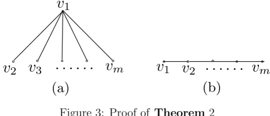
Figure 3: Proof of Theorem 2
multiple attributes, and retaining only dependency in at most a single attribute at a time,
which results in a tree-like structure. It is easy to see that in the fully connected weighted
graph G, there are a large number of trees, each of which represents a unique approximation
dependency structure. Here, in order to reduce the uncertainty in the dataset and maximize
the mutual information among the attributes simultaneously, we find the minimum spanning
tree as our best dependency tree from the fully connected graph G based on our proposed
mutual information measure. Here, we use the Kruskal algorithm [6], which is essentially a
greedy algorithm. The candidate edges are sorted in increasing order of their weights (i.e.
mutual information measure). Then, starting with an empty set E0, the algorithm examines
one edge at a time (in the order resulting from the sort operation), checks if it forms a cycle
with the edges already in E0 and, if not, adds it toE0. The algorithm ends whenm−1 edges
Algorithm 1: Finding best dependency tree
1. Compute the mutual information measure between
each pair of attributes in T and construct the dependency
matrix DT. There arem(m−1)/2 weight need to be
calculated, since T has m attributes.
2. Construct a fully connected graph, where the nodes
correspond to the attributes in T. The weight of each edge
refers to their mutual information measure.
3. Find the best dependency tree by the the minimum spanning tree algorithm.
The algorithm of finding best dependency tree is briefly described in Algorithm 1 and an
example of the found out best dependency tree is shown in Figure 2(Right).
After finding out the best dependency tree, we need to set out rules to select the key
attributes from the dependency tree to process approximate microaggregation.
Definition 4 (Degree of The Vertex). LetG= (V, E)be a graph, whereV ={v1, v2,· · · , vm}.
Then, the degree of the nodevi is the number of edges incident to the nodes, denoted bydeg(vi).
For example, in Figure 2(Right), deg(A2) = 4, and deg(A3) = 2. Let TG be the best
dependency tree found inG. We then compute the degree of each vertex inTG and sort them
in decreasing order. Without loss of generality, we assume that deg(v1) ≥ deg(v2) ≥ · · · ≥
deg(vm) after they are sorted in decreasing order. Then, the principle of choosing the key
attributes is as follows:
Definition 5 (Choosing Key Attributes). Suppose deg(v1) ≥ deg(v2) ≥ · · · ≥ deg(vm)
after they are sorted. Then, the vertices v1, v2,· · ·vk are chosen as the key attributes if the
Algorithm 2: k-anonymity through approximate microaggregation Input: Microdata set T consisting ofn records havingm attributes each. Output: Microaggregated microdataT′ satisfying k-anonymity property
1. Find out the best dependency tree by Algorithm 1 and select the key attributes
2. Project the records ofT to the key attributes.
3. Computes the centroid (average record) ¯x of records in the projected data set, and find the most distant recordr from the centroid and the most distant record sfromr.
4. Form two groups aroundr and s: the first group containsr and thek−1 records closest tor; The other group containss and thek−1 records closest tos.
5. If there are at least 2krecords which do not belong to any of the groups formed in Step 4, go to Step 3, taking the previous set of records minus the groups formed in the latest instance of Step 4, as the new set of records.
6. If there are betweenk and k−1 records which do not belong to any of the groups formed in Step 4, form a new group with those records and exit the algorithm.
7. If there are less thank remaining records which do not belong to any of the groups formed in Step 4, add them to the group formed in Step 4 whose centroid is closest to the centroid of the remaining records.
8. Return microaggregated dataT′ by replacing each record by the centroid of the group it belongs to.
k−1
∑
i=1
deg(vi)< m (11)
k
∑
i=1
deg(vi)≥m (12)
For example, for the minimum spanning treeTG in Figure 2, we choose attributes A2 and
A3 as the key attributes, since according to the principle described above, deg(A2) <6 and
deg(A2) +deg(A3) = 6.
Theorem 2: Let TG be the best dependency tree of G, with V = {v1, v2,· · · , vm}, and N be
Proof: Since in a tree-like structure, the maximum degree of a vertex ism−1 [6], and without
loss of generality, we assume that deg(v1) = m−1, and in this case, the best dependency
tree found has the form as shown in Figure 3(a), and then according to Definition 5, only
two vertices will be selected as key attributes, say v1 and v2. This is the situation when
the number of the selected key attributes reaches the minimality. On the other hand, when
the number of the selected key attributes reaches the maximality, the structure of the best
dependency tree has the form as shown in Figure 3(b), and in this case, at most m/2 key
attributes will be selected. So, 2 ≤N ≤m/2.
Theorem 2 assures that at most half the amount of dimension resources are needed in the
microaggregation process with our technique, which could significantly reduce the execution
time. In the next section, we discuss in detail how to apply this technique to k-anonymity
problem.
3.3
Application to
K
-Anonymity
Our aim is to obtain k-anonymous microdata without coarsened nor partially suppressed
data. This makes their analysis and exploitation easier, with the additional advantage that
numerical continuous attributes are not categorized. In this section, we adopt the approximate
microaggregation technique to solve k-anonymity problem.
Our algorithm receives as input a microdata set T consisting of n records having m
at-tributes each. The result of the algorithm is ak-partition used to microaggregate the original
microdata set and to generate a microaggregated data set T′ that fulfils the k-anonymity
property. Instead of taking all the attributes into the microaggregation process, we only use the selected key attributes, which captures the dependency between attributes, to
microag-gregate the data. The novelty and difference from the previous microaggregation methods
exist here. Our proposed approach is effective and efficient in terms of running time and
information loss.
The first two steps of the algorithm builds the initial dataset for microaggregation. It
selects the key attributes from the best dependency tree and returns a projected dataset,
attributes. Once the average record is computed, the algorithm looks for other records which
are distant to it and adds records to it until it reaches a minimum cardinality k (Step
3-4). After repeating this process several times, a set of groups satisfying the k-anonymity
property is obtained. However, a number of records can remain unassigned, and they must be
distributed amongst the previously created groups (Step 5-7). Finally, the algorithm further
microaggregates the original microdataT by replacing each record inT by the centroid of the
group to which it belongs (Step 8). The algorithm is outlined in Algorithm 2.
In this section, we discuss in detail how to apply our microaggregation technique to solve
k-anonymity in order to overcome most of the problems of generalization/suppression listed
in Section 2 in the following aspects:
• Approximate microaggregation is a unified approach, unlike the dual method combining
generalization and suppression.
• It does not complicate data analysis by adding new categories to the original scale, unlike
generalization/suppression.
• It does not result in suppressed data, which makes analysis of k-anonymous data easy.
• It is suitable to protect continuous data without removing their numerical semantics.
4
Experimental Results
4.1
Data set
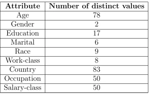
We employ a real-life CENSUS data set downloadable at http://www.ipums.org in the
ex-perimental study. The CENSUS data set contains the personal information of 500K American
adults. The data set has 9 discrete attributes summarized in Table 4. From CENSUS, we
create two sets of micro tables, in order to examine the influence of dimensionality and the
impact of cardinality. The first set has 6 tables, denoted as CENSUS-20%, · · ·,
CENSUS-100%, respectively. Specifically, CENSUS-t% (20≤t≤100) indicates the data set consisting
Attribute Number of distinct values
Age 78
Gender 2
Education 17
Marital 6
Race 9
Work-class 8
Country 83
Occupation 50
Salary-class 50
Table 4: Summary of attributes in CENSUS
attributes shown in Table 4. The second set contains 5 tables, denoted as 5-CENSUS, · · ·,
9-CENSUS, respectively, where n-CENSUS (3≤n≤9) represents the data set with the first
n attributes selected from Table 4, and each data set has the same number of records as the
whole CENSUS data set.
4.2
Experiment setup
Our aim is to test the efficiency and effectiveness of the proposed approximate
microaggrega-tion algorithm for k-anonymity. We denote our proposed algorithm asM A, and we compare
it with the previous MDAV-based algorithm [11], denoted as M A. We first evaluate the
execution time of our approach by varying the cardinality of the data sets, the number of
attributes and the value of k. In order to compare the effectiveness, for each data set, we
adopt two measurements. One is to measure the information loss in terms of SSE/SST,
where SSE is the sum of square errors as defined in equation (1), andSST refers to the sum
of square errors applied over the whole dataset. The other metric is to compare the number
of key attributes projected in the microaggregation.
4.3
Results
Efficiency: Figures 4(a)-(c) show the comparison of execution time of two microaggregation
Census−20%10 Census−40% Census−60% Census−80% Census−100% 20 30 40 50 60
Running time (Sec)
MA AMA
(a)
K=5 K=10 K=15 K=20 K=25 0 10 20 30 40 50 60 70 80
Running time (Sec)
MA AMA
(b)
5−Census 6−Census 7−Census 8−Census 9−Census 20 25 30 35 40 45 50 55 60
Running time (Sec)
AMA MA
(c)
Figure 4: Running time comparison between different methods
4(a) plots the result by varying the data percentage of the whole Census data set from
20% to 100%. As we can see, the AMA incurs less computation time than MA method. This is expected since in the AMA process, less attributes are used in the microaggregation.
We can see the difference of the computation cost is getting larger with the increased data
cardinality. Figure 4(b) describes the running time comparison when varying the privacy
parameter k. The computation cost of both MA and AMA algorithms is increasing with k,
but AMA consistently outperforms MA method. Figure 4(c) shows the computation overhead
differences by altering the number of attributes. The computation overhead of both methods
is increasing when enlarging the number of attributes. The result is expected since the
overhead is increased with the more dimensions. The AMA method performs better than MA
algorithm since we use a part of the attributes instead of the whole dimensional resources, which is significantly reduce the amount of computation.
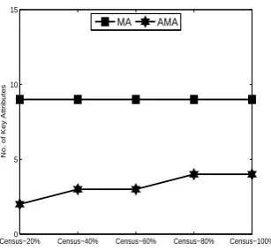
Effectiveness: Having verified the efficiency of our technique, we proceed to test its
effective-ness. We measure the utility in terms of SSE/SST, where SSE is the sum of square errors
as defined in equation (1), and SST refers to the sum of square errors applied over the whole
data set. Figure 5 shows the number of key attributes used in MA and AMA approaches. As
we can see, the number remains the same for MA method, since it projects all the attributes
Census−20%0 Census−40% Census−60% Census−80% Census−100% 5
10 15
No. of Key Attributes
MA AMA
Figure 5: No. of key attributes comparison
AMA is less than half of that used by MA approaches, which verifies the results in Theorem 2.
Figures 6(a) and (b) show the information loss by applying MA and AMA algorithms.
Figure 6(a) is plotted by changing the percentage of data set. Although the result indicates
that AMA generates a little bit more information loss than MA, the difference is not enlarged
when the data cardinality is increased. Similar tread is obtained in Figure 6(b) by varying the
value k. The information loss is increased with k, since larger k demands more strict privacy
requirement, which reduces the utility of the data.
Summary: Overall, the AMA outperforms MA in terms of efficiency, and the difference
is getting larger when the volume and dimension of data are increasing. Although AMA generates a little bit more information loss than MA, it is still practical since AMA only uses
at most half of the attributes in the microaggregation process.
5
Related Work
Privacy preservation is an important issue in the release of data for mining purpose. The k
-anonymity model, which was introduced for protecting individual identification by Samarati
and Sweeney [29, 31], has been extensively investigated for its simplicity and effectiveness
Census−20% Census−40% Census−60% Census−80% Census−100% 0
10 20 30 40 50 60
Information Loss
AMA MA
(a)
K=5 K=10 K=15 K=20 K=25 20
30 40 50 60 70
Information loss
MA AMA
(b)
Figure 6: Information loss comparison between different methods
be indistinguishable with at leastk−1 other records within the dataset with respect to a set of
quasi-identifier attributes. In this case, individuals cannot be uniquely identified by adversary, so the individuals’ privacy can be preserved. Started from [29, 31, 30], the general approach
adopted in the literature to achievek-anonymity is based on generalization/suppression, which
has some defects on efficiency, information loss and implementation. Our work in this paper
is related to the microaggregation technique, which has been introduced to implement k
-anonymous data set recently and remedies most of defects of generalization and suppression
[12, 10, 11, 22, 9].
In the previous research, all the dimensional resources (attributes) are required in the
microaggregation process. However, as mentioned in [10, 11, 9], the result and execution
time of the microaggregation highly depends on the number of the variables used in the mi-croaggregation process, since few variables sometimes offers the better solutions. Different
from previous microaggregation methods, in this paper, we propose a new approach to select
only a small number of dimensional resources that captures the maximal dependency
rela-tionship among resources and as experiments show that the new technique achieves better
microaggregation results. Specifically, our microaggregation method is effective and efficient
in terms of information loss and running time. In the case of k-anonymity problem, the
generalization/suppression. (1) Our method is a unified approach, unlike the dual method
combining generalization and suppression. (2) It does not complicate data analysis by adding
new categories to the original scale, unlike generalization/suppression. (3) It does not result in
suppressed data, which makes analysis ofk-anonymous data easy. (4) It is suitable to protect
continuous data without removing their numerical semantics. From a different perspective,
the microaggregation technique discussed in this paper produces better solutions compared
with previous ones.
Our work is also related to the application of dependency tree of information theory
in data mining and databases. The dependency tree has been used in finding dependency
structure in the features which improve the classification accuracy of the Bayes network
classifiers [14]. [5] uses the dependency tree to represent a set of frequent patterns, which can
be used to summarize patterns into few profiles. [17] presents large node dependency tree,
in which the nodes are subsets of variables of data set. The large node dependency tree is
applied to density estimation and classification. As far as its application to privacy preserving
data mining, fewer results are obtained. In this paper, we introduce the concept of entropy
and propose the mutual information measure to evaluate the mutual dependency between attributes, and the method to construct the dependency tree. We also discuss how to select
key attributes from the constructed dependency tree, and how to use them in the approximate
microaggregation. We prove theoretically that at most half the amount of resources are needed
with our approach.
6
Conclusion and Future Work
k-anonymity is a property that, when satisfied by the microdata, can help increase the privacy
of the respondents whose data is being used. Previous approaches to obtain microdata sets
fulfilling the k-anonymity property were mainly based on suppression and generalization.
In this article, we have shown how to achieve the same property by means of approximate
microaggregation, which, different from the previous microaggregation method, uses a part of
the dimensional resources. It works by selecting key attributes from the best dependency tree,
which captures the dependency between attributes in the microdata. The experimental results
show that the proposed technique is efficient and effective in the terms of running time and
information loss.
A number of other sophistication ofk-anonymity for protecting against attribute disclosure
have recently been proposed, such as (p+, α)-sensitivek-anonymity [37],l-diversity [20], (α, k
)-anonymity [39], t-closeness [19]. All of them rely on generalizations, so the microaggregation
approach proposed in this paper would be a novelty in all of them. The technique proposed in this paper restricted its focus on numerical attributes, and it is interesting to investigate
the extension to other types of attributes.
References
[1] G. Aggarwal, T. Feder, K. Kenthapadi, R. Motwani, R. Panigrahy, D. Thomas and A.
Zhu. Anonymizing tables. In Proc. of the 10th International Conference on Database Theory
(ICDT’05), pp. 246-258, Edinburgh, Scotland.
[2] C. Boyens, R. Krishnan, and R. Padman. On privacy-preserving access to distributed
het-erogeneous healthcare information. In I. C. Society, editor, Proceedings of the 37th Hawaii
International Conference on System Sciences HICSS-37, Big Island, HI., 2004.
[3] R. Brand, J. Domingo-Ferrer, and J. M. Mateo-Sanz, Reference data sets to test and compare
sdc methods for protection of numerical microdata, 2002, European Project IST-2000-25069
CASC,http://neon.vb.cbs.nl/casc.
[4] C. Chow and C. Liu. Approximating discrete probability distributions with dependence trees.
IEEE Transactions on Information Theory, 14,3:462-467, 1968.
[5] G. Cong, B. Cui, Y. Li, and Z. Zhang. Summarizing frequent patterns using profiles.In Database
Systems for Advanced Applications, 11th International Conference, DASFAA, 2006.
[6] T. Cormen, C. Leiserson, R. Rivest, C. Stein.Introduction to Algorithms, second edition, MIT
Press and McGraw-Hill. ISBN 0-262-53196-8.
[7] Data lost by Revenue and Customs. BBC News.http://news.bbc.co.uk/1/hi/uk/7103911.
[8] D. Defays and P. Nanopoulos, Panels of enterprises and confidentiality: the small aggregates
method, in Proc. of 92 Symposium on Design and Analysis of Longitudinal Surveys. Ottawa:
Statistics Canada, 1993, pp. 195-204.
[9] J. Domingo-Ferrer, V. Torra. Aggregation Techniques for Statistical confidentiality. In:
Aggre-gation operators: new trends and applications, pp. 260-271. Physica-Verlag GmbH, Heidelberg
(2002)
[10] J. Domingo-Ferrer and V. Torra, On the connections between statistical disclosure control for
microdata and some artificial intelligence tools, Information Sciences, vol. 151, pp. 153-170,
May 2003.
[11] J. Domingo-Ferrer and J. M. Mateo-Sanz, Practical data-oriented microaggregation for
statis-tical disclosure control,IEEE Transactions on Knowledge and Data Engineering, vol. 14, no. 1,
pp. 189-201, 2002.
[12] J. Domingo-Ferrer and V. Torra, Ordinal, continuous and heterogenerousk-anonymity through
microaggregation, Data Mining and Knowledge Discovery, vol. 11, no. 2, pp. 195-212, 2005.
[13] E. C. for Europe, Statistical data confidentiality in the transition countries: 2000/2001 winter
survey, in Joint ECE/Eurostat Work Session on Statistical Data Confidentiality, 2001, invited
paper n.43.
[14] N. Friedman, D. Geiger, and M. Goldszmid. Bayesian network classifiers. Machine Learning,
29:131-163, 1997.
[15] S. Hansell. AOL removes search data on vast group of web users. New York Times, Aug 8 2006.
[16] HIPAA. Health insurance portability and accountability act, 2004.http://www.hhs.gov/ocr/
hipaa/.
[17] K. Huang, I. King, and M. Lyu. Constructing a large node chow-liu tree based on frequent
itemsets. In Proceedings of the International Conference on Neural Information Processing,
2002.
[18] K. LeFevre, D. DeWitt, and R. Ramakrishnan. Incognito: Efficient Full-Domain k-Anonymity.
[19] N. Li, T. Li and S. Venkatasubramanian. t-Closeness: Privacy Beyond k-anonymity and
l-diversity.ICDE 2007: 106-115
[20] A. Machanavajjhala, J. Gehrke, D. Kifer, and M. Venkitasubramaniam. l-Diversity: Privacy
beyond k-anonymity.ICDE 2006.
[21] A. Meyerson and R. Williams. On the complexity of optimal k-anonymity.In Proc. of the 23rd
ACM-SIGMOD-SIGACT-SIGART Symposium on the Principles of Database Systems, pp.
223-228, Paris, France, 2004.
[22] A. Oganian and J. Domingo-Ferrer, On the complexity of optimal microaggregation for
sta-tistical disclosure control, Statistical Journal of the United Nations Economic Comission for
Europe, vol. 18, no. 4, pp. 345-354, 2001.
[23] Euro. Parliament. DIRECTIVE 2002/58/EC of the European Parliament and Council of 12 july
2002 concerning the processing of personal data and the protection of privacy in the electronic
communications sector (Directive on privacy and electronic communications), 2002. http://
europa.eu.int/eur-lex/pri/en/oj/dat/2002/l_201/l_20120020731en00370047.pdf.
[24] E. Pfanner. Data Leak in Britain Affects 25 Million. The New York Times. http://www.
nytimes.com/2007/11/22/world/europe/22data.html, November 22, 2007.
[25] M. Rosemann, Erste Ergebnisse von vergleichenden Untersuchungen mit anonymisierten und
nicht anonymisierten Einzeldaten am Beispiel der Kostenstrukturerhebung und der
Umsatzs-teuerstatistik, in G. Ronning and R. Gnoss (editors), Anonymisierung wirtschaftsstatistischer
Einzeldaten, Wiesbaden: Statistisches Bundesamt, 2003, pp. 154-183.
[26] Ca. Privacy. Canadian privacy regulations, 2005.http://www.media-awareness.ca/english/
issues/privacy/canadian_legislation_privacy.cfm.
[27] US. Privacy. U.S. privacy regulations, 2005. http://www.media-awareness.ca/english/
issues/privacy/us_legislation_privacy.cfm.
[28] Aus. Privacy. Review of Australian Privacy Law, Discussion Paper 72, (DP 72), September
[29] P. Samarati and L. Sweeney. Protecting privacy when disclosing information: k-anonymity and
its enforcement through generalization and suppression.Technical Report SRI-CSL-98-04, SRI
Computer Science Laboratory, 1998.
[30] P. Samarati. Protecting respondents’ identities in microdata release. IEEE Transactions on
Knowledge and Data Engineering, 13(6): pp: 1010-1027. 2001.
[31] P. Samarati. and L. Sweeney. Generalizing data to provide anonymity when disclosing
infor-mation (Abstract). In Proc. of the 17th ACM-SIGMODSIGACT- SIGART Symposium on the
Principles of Database Systems, p. 188, Seattle, WA, USA, 1998.
[32] A. Solanas and A. Martinez-Balleste, A Multivariate Microaggregation With Variable Group
Size.In 17th COMPSTAT Symposium of the IASC, Rome (2006).
[33] A. Solanas and A. Martinez-Balleste. Privacy protection in location-based services through a
public-key privacy homomorphism.In EuroPKI’07,LNCS 4582, pages 362-368. Springer, June
2007
[34] A. Solanas, J. Domingo-Ferrer, A. Martinez-Balleste and V. Daza. A Distributed Architecture
for Scalable RFID Identification. Computer Networks, 51, 2007
[35] X. Sun, M. Li, H. Wang and A. Plank. An efficient hash-based algorithm for minimal
k-anonymity problem. 31st Australasian Computer Science Conference (ACSC 2008),
Wollon-gong, NSW, Australia. CRPIT 74, pp: 101-107.
[36] X. Sun, H. Wang and J. Li. On the complexity of restricted k-anonymity problem. 10th Asia
Pacific Web Conference (APWeb 2008), LNCS 4976, pp: 287-296, Shenyang, China.
[37] X. Sun, H. Wang, J. Li, T. M. Traian and P. Li. (p+, α)-sensitivek-anonymity: a new enhanced privacy protection model.In 8th IEEE International Conference on Computer and Information
Technology (IEEE-CIT 2008), 8-11 July 2008, Sydney, Australia. pp:59-64.
[38] L. Sweeney. Achieving k-anonymity privacy protection using generalization and suppression.
International Journal on Uncertainty, Fuzziness, and Knowledge-based Systems, 10(5):571-588,
2002.
[39] R. Wong, J. Li, A. Fu, K. Wang. (α, k)-anonymity: an enhancedk-anonymity model for privacy