Spatial clustering method for geographic data

(1)

CENTRE FOR

ADV

ANCED

SP

A

TIAL

ANAL

YSIS

W

orking Paper Series

Paper 41

SPATIAL

CLUSTERING

METHOD FOR

GEOGRAPHIC

DATA

(2)

Centre for Advanced Spatial Analysis University College London

1-19 Torrington Place Gower Street

London WC1E 6BT

[t] +44 (0) 20 7679 1782 [f] +44 (0) 20 7813 2843 [e] [email protected]

[w] www.casa.ucl.ac.uk

http//www.casa.ucl.ac.uk/paper41.pdf

Date: January 2002

ISSN: 1467-1298

Toshihiro Osaragi

Toshihiro Osaragi is an Associate Professor in the Graduate School of Information Science and Engineering at Tokyo Institute of Technology. He was an Academic Visitor at the Centre for Advanced Spatial Analysis from March 2001 to January 2002.

Department of Mechanical and Environmental Informatics Graduate School of Information Science and Engineering Tokyo Institute of Technology

2-12-1 O-okayama, Meguro-ku, Tokyo 152-8552, JAPAN Tel:+81-3-5734-3162 Fax:+81-3-5734-2817

(3)

Spatial Clustering Method for Geographic Data

Toshihiro OSARAGI

Abstract: In the process of visualizing quantitative spatial data, it is necessary to classify attribute values into some class divisions. In a previous paper, the author proposed a classification method for minimizing the loss of information contained in original data. This method can be considered as a kind of smoothing method that neglects the characteristics of spatial distribution. In order to understand the spatial structure of data, it is also necessary to construct another smoothing method considering the characteristics of the distribution of the spatial data. In this paper, a spatial clustering method based on Akaike’s Information Criterion is proposed. Furthermore, numerical examples of its application are shown using actual spatial data for the Tokyo Metropolitan area.

Keywords: spatial data, space cluster, Quadtree, AIC (Akaike’s Information Criterion), information loss, visualization, classification

1. Introduction

When spatial data are visualized, the attribute values defined numerically have to be classified into some class divisions. In this process, there exists the risk of leading us to miss-judgment or biased understanding, since much information of the original data may be lost, according to the classification method adopted. Therefore, in a previous paper, Osaragi (2001) examined the classification method of spatial data from the viewpoint of information-statistics, and proposed a new classification method based on minimization of information loss. This method is a sort of smoothing technique neglecting the characteristics of spatial data distribution. However, it is necessary to consider the spatial distribution of attributes, to adequately visualize data accompanied with information of "spatial distribution".

(4)

presented a numerical method for classifying geographic data in order to incorporate geographic location as an external constraint. Once the matrix of similarity values has been generated and the adjacency coded, a hierarchical agglomerative fusion strategy can be used to construct hierarchical relationships between the objects (Margules et al. 1985). Conversely, Batty (1974, 1976, 1978) discussed the zonal aggregation problem according to a spatial entropy scaled for zone size, and decomposed the information gain into a within-set and a between-set component.

Furthermore, Fotheringham and Wong (1991) has suggested that the sensitivity of analytical results to the definition of units for which data are collected. This stubborn problem related to the use of areal data is commonly referred to as the modifiable areal unit problem (MAUP), which is clearly illustrated through the works of Openshaw and Taylor (1979). Although any specific statistical analysis is usually not employed in the process of visualizing spatial data, the results are likely to vary with the level of aggregation and with the configuration of the zoning system. Then we have to consider appropriate areal units in this process.

In this paper, we discuss a spatial clustering method considering the characteristics of the local spatial distribution of attributes. Namely, we discuss the question "Which places should be unified as a spatial unit in the sense of a statistical model?" In the following, such a spatial unit is called "space-cluster". Tamagawa (1987) and Higuchi et al. (1988) have proposed a method for deciding the optimum cell-size in which the values of AIC (Akaike’s Information Criterion; Akaike 1972, 1974), obtained thorough variously changing the observed range of data, are compared. Furthermore, Nakaya (2000) has also proposed a methodology to select appropriate areal units using AIC and search methods for an informative geographical aggregation in map construction. In this paper, combining these ideas with our spatial classifying and visualizing method, a new spatial clustering method for geographical data is proposed.

2. Definition of Space-cluster

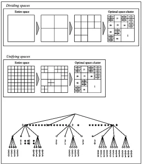
When asking for the appropriate space-cluster, we have two options. The first is to make each space-cluster a uniform size. The second is to change the size of every space-cluster if needed. In this paper, the way of the latter, with higher flexibility than the former, is attempted. That is, we examine how to represent the entire space by a set of space-clusters of various sizes. The fundamental idea is as follows.

(5)

the area into some smaller sub-areas. Furthermore, checking the homogeneity of feature distribution in the sub-areas, further division within each sub-area will be done anew, if necessary. The entire study area is divided by repeating this procedure. Thus, if it becomes unnecessary to divide sub-areas any further, i.e., if each sub-area can be statistically considered homogeneous, it can be considered that the objective area is filled with appropriate space-clusters at this time. Even if the sub-areas are divided into smaller sub-areas further, we can get only a little information from the data, and the data size will be getting large. That is, we should pay attention to the trade-off relationship between amount of information and amount of data itself.

According to the above discussion, the space-cluster is obtained by a dividing process. However, it is also possible to constitute a space-cluster by unifying smaller sub-areas (see figure 1). According to the author’s experience, the latter option is able to constitute a finer space-cluster than the former one. The concrete reason for this will be shown later.

Optimal space-cluster Entire space Optimal space-cluster Entire space Dividing spaces Unifying spaces 1 01 02 032 033

030 031 322 323 320 321 222 223 220 221

312 313 310 311

20 21 23 30 1 01 02

002 003 000 001 002 003 000 001

032 033 030 031 032 033 030 031

322 323 320 321 322 323 320 321

332 333 330 331 220 221

220 221

20 21 30

1

01 02 032 033

030 031 322 323 320 321 222 223 220 221

312 313 310 311

20 21 23 30 1 01 02

002 003 000 001 002 003 000 001

032 033 030 031 032 033 030 031

322 323 320 321 322 323 320 321

332 333 330 331 220 221

220 221

20 21 30

0 @ @ @ @ @ @ @ @1 @ @ @ @ @ @ 2 @ @ @ @ @ @ @ @ @ @3

0 @ @0 @ 2 2 2 3

1 @ @2 @ 0 1 3 0

0 0 0 0 0 0 0 0 0 1 2 3

0 0 0 0 3 3 3 3 0 1 2 3

0 0 0 0 0 0 0 0 0 1 2 3

0 @ @ @ @ @ @ @ @1 @ @ @ @ @ @ 2 @ @ @ @ @ @ @ @ @ @3

0 @ @0 @ 2 2 2 3

1 @ @2 @ 0 1 3 0

0 0 0 0 0 0 0 0 0 1 2 3

0 0 0 0 3 3 3 3 0 1 2 3

0 0 0 0 0 0 0 0 0 1 2 3

0 @ @ @ @ @ @ @ @1 @ @ @ @ @ @ 2 @ @ @ @ @ @ @ @ @ @3

0 @ @0 @ 2 2 2 3

1 @ @2 @ 0 1 3 0

0 0 0 0 0 0 0 0 0 1 2 3

0 0 0 0 3 3 3 3 0 1 2 3 0 0 0 0

0 0 0 0 0 1 2 3

0 0 0 0 3 3 3 3 0 1 2 3

0 0 0 0 0 0 0 0 0 1 2 3 0 0 0 0 0 0 0 0 0 1 2 3

0 0 0 0 0 0 0 0 0 1 2 3

0 0 0 0 0 0 0 0 0 1 2 3 0 0 0 0

0 0 0 0 0 1 2 3

0 0 0 0 0 0 0 0 0 1 2 3

0 0 0 0 0 0 0 0 0 1 2 3 Optimal space-cluster

Entire space Optimal space-cluster

Entire space

Optimal space-cluster

Entire space Optimal space-cluster

Entire space

Dividing spaces

Unifying spaces

1

01 02 032 033

030 031 322 323 320 321 222 223 220 221

312 313 310 311

20 21 23 30 1 01 02

002 003 000 001 002 003 000 001

032 033 030 031 032 033 030 031

322 323 320 321 322 323 320 321

332 333 330 331 220 221

220 221

20 21 30

1

01 02 032 033

030 031 032 033 030 031

322 323 320 321 322 323 320 321 222 223 220 221 222 223 220 221

312 313 310 311 312 313 310 311

20 21 23 30 1 01 02

002 003 000 001 002 003 000 001

032 033 030 031 032 033 030 031

322 323 320 321 322 323 320 321

332 333 330 331 220 221

220 221

20 21 30

1

01 02 032 033

030 031 322 323 320 321 222 223 220 221

312 313 310 311

20 21 23 30 1 01 02

002 003 000 001 002 003 000 001

032 033 030 031 032 033 030 031

322 323 320 321 322 323 320 321

332 333 330 331 220 221

220 221

20 21 30

1

01 02 032 033

030 031 032 033 030 031

322 323 320 321 322 323 320 321 222 223 220 221 222 223 220 221

312 313 310 311 312 313 310 311

20 21 23 30 1 01 02

002 003 000 001 002 003 000 001

032 033 030 031 032 033 030 031

322 323 320 321 322 323 320 321

332 333 330 331 220 221

220 221

20 21 30

0 @ @ @ @ @ @ @ @1 @ @ @ @ @ @ 2 @ @ @ @ @ @ @ @ @ @3

0 @ @0 @ 2 2 2 3

1 @ @2 @ 0 1 3 0

0 0 0 0 0 0 0 0 0 1 2 3

0 0 0 0 3 3 3 3 0 1 2 3

0 0 0 0 0 0 0 0 0 1 2 3

0 @ @ @ @ @ @ @ @1 @ @ @ @ @ @ 2 @ @ @ @ @ @ @ @ @ @3

0 @ @0 @ 2 2 2 3

1 @ @2 @ 0 1 3 0

0 0 0 0 0 0 0 0 0 1 2 3

0 0 0 0 3 3 3 3 0 1 2 3

0 0 0 0 0 0 0 0 0 1 2 3

0 @ @ @ @ @ @ @ @1 @ @ @ @ @ @ 2 @ @ @ @ @ @ @ @ @ @3

0 @ @0 @ 2 2 2 3

1 @ @2 @ 0 1 3 0

0 0 0 0 0 0 0 0 0 1 2 3

0 0 0 0 3 3 3 3 0 1 2 3 0 0 0 0

0 0 0 0 0 1 2 3

0 0 0 0 3 3 3 3 0 1 2 3

0 0 0 0 0 0 0 0 0 1 2 3 0 0 0 0 0 0 0 0 0 1 2 3

0 0 0 0 0 0 0 0 0 1 2 3

0 0 0 0 0 0 0 0 0 1 2 3 0 0 0 0

0 0 0 0 0 1 2 3

0 0 0 0 0 0 0 0 0 1 2 3

0 @ @ @ @ @ @ @ @1 @ @ @ @ @ @ 2 @ @ @ @ @ @ @ @ @ @3

0 @ @0 @ 2 2 2 3

1 @ @2 @ 0 1 3 0

0 0 0 0 0 0 0 0 0 1 2 3

0 0 0 0 3 3 3 3 0 1 2 3

0 0 0 0 0 0 0 0 0 1 2 3

0 @ @ @ @ @ @ @ @1 @ @ @ @ @ @ 2 @ @ @ @ @ @ @ @ @ @3

0 @ @0 @ 2 2 2 3

1 @ @2 @ 0 1 3 0

0 0 0 0 0 0 0 0 0 1 2 3

0 0 0 0 3 3 3 3 0 1 2 3 0 0 0 0

0 0 0 0 0 1 2 3

0 0 0 0 3 3 3 3 0 1 2 3

0 0 0 0 0 0 0 0 0 1 2 3 0 0 0 0 0 0 0 0 0 1 2 3

0 0 0 0 0 0 0 0 0 1 2 3

0 0 0 0 0 0 0 0 0 1 2 3 0 0 0 0

0 0 0 0 0 1 2 3

0 0 0 0 0 0 0 0 0 1 2 3

0 @ @ @ @ @ @ @ @1 @ @ @ @ @ @ 2 @ @ @ @ @ @ @ @ @ @3

0 @ @0 @ 2 2 2 3

1 @ @2 @ 0 1 3 0

0 0 0 0 0 0 0 0 0 1 2 3

0 0 0 0 3 3 3 3 0 1 2 3 0 0 0 0

0 0 0 0 0 1 2 3

0 0 0 0 3 3 3 3 0 1 2 3

0 0 0 0 0 0 0 0 0 1 2 3 0 0 0 0 0 0 0 0 0 1 2 3

0 0 0 0 0 0 0 0 0 1 2 3

0 0 0 0 0 0 0 0 0 1 2 3 0 0 0 0

0 0 0 0 0 1 2 3

0 0 0 0 0 0 0 0 0 1 2 3

0 @ @ @ @ @ @ @ @1 @ @ @ @ @ @ 2 @ @ @ @ @ @ @ @ @ @3

0 @ @0 @ 2 2 2 3

1 @ @2 @ 0 1 3 0

0 0 0 0 0 0 0 0 0 1 2 3

0 0 0 0 3 3 3 3 0 1 2 3 0 0 0 0

0 0 0 0 0 1 2 3

0 0 0 0 3 3 3 3 0 1 2 3

0 0 0 0 0 0 0 0 0 1 2 3 0 0 0 0 0 0 0 0 0 1 2 3

0 0 0 0 0 0 0 0 0 1 2 3

0 0 0 0 0 0 0 0 0 1 2 3 0 0 0 0

0 0 0 0 0 1 2 3

0 0 0 0 0 0 0 0 0 1 2 3

(6)

Margules et al. (1985) tested four agglomerative hierarchical fusion strategies with the adjacency constraint. The choice of classification strategy, which should depend on the type and amount of data and objective of the classification, is an important decision that applies equally to constrained or unconstrained classification. In this research, the Quadtree data structure is used for the process of finding the optimal space-cluster. The applications discussed here are limited to the Quadtree data structure. However, the following method can be applied to any other fusion strategies or data structures. Figure 1 shows an example in which an appropriate space-cluster is expressed using the Quadtree structure. Assuming the top level is the entire study area, the low rank can be considered sub-areas. Furthermore, each leaf can be considered the smallest sub-area, i.e., a space-cluster. That is, an adequate space-cluster can be obtained by traversing the tree using an evaluation function.

3. Space-cluster based on AIC

3.1 Definition of AIC

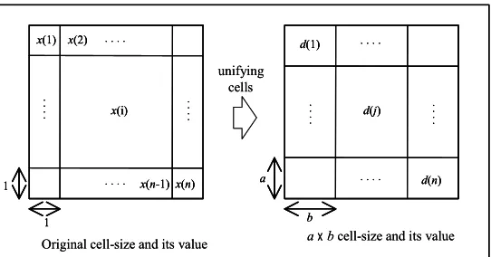
Tamagawa (1987) and Higuchi et al. (1988) proposed a method based on AIC in order to determine the optimum cell-size. A function of AIC was formulated as follows, transforming the whole area into uniform cell-size (see figure 2). The attribute value of a unit cell is denoted by x (i), (i=1, 2,…,

n), and the sum of values in the entire area is denoted by X (

∑

=

= n

i

i x

1

)

( ). Furthermore, horizontal

width and vertical height are represented by a and b respectively when changing cell-size. Furthermore, an attribute value of an axb-cell is denoted by d(j),(j=1, 2, ..., N). As for the data with which the attribute value is defined as a discrete value like point sampling data, the value of AIC can be described as follows:

) 1 ( 2 ) ( log ) ( 2 AIC

1 ⋅ + −

−

=

∑

= abX N

j d j d

N j

, (1)

where ( )⋅log ( )=0 abX

j d j

(7)

Original cell-size and its value

d(1)

d(n) . . . .

. . . . d(j)

a

b

. . .

.

. .

.

x(1) x(2)

x(n-1)x(n) . . . .

. . . . x(i)

1

. .

.

. .

a bcell-size and its value unifying

cells

Original cell-size and its value

d(1)

d(n) . . . .

. . . . d(j)

a

b

. . .

.

. .

.

d(1)

d(n) . . . .

. . . . d(j)

a

b

. . .

.

. .

.

x(1) x(2)

x(n-1)x(n) . . . .

. . . . x(i)

1

. .

.

. .

x(1) x(2)

x(n-1)x(n) . . . .

. . . . x(i)

1

. .

.

. .

a bcell-size and its value unifying

cells

Figure 2: Cell-size and attribute values

Furthermore, in the case of data with which attribute values are defined as a continuous value like a ratio, the value of AIC is defined as follows:

) 1 ( 2 ˆ

log 2

log

AIC₌_n

_π

₊_n

_σ

2₊_n₊ _N₊ _, ₍₂₎

where _

  

 

−

=

∑

= =

N j n

i ab

j d i x

n 1

2

1 2

2 1 ₍₎ ( )

ˆ

σ

.

The cell-size that gives the minimum value of AIC can be regarded as optimal, in a sense of the trade-off relationship between amount of information and amount of data. However, this method is based on the idea of covering the entire area by the same-sized cells.

The author proposes a method for obtaining the optimal space-cluster using the evaluation function of AIC. The fundamental procedure is shown in figure 3. By unifying four sub-areas belonging to the same tree, whose size is 2k_{, the new sub-area whose size is 2}k+1_{is formed. Here, the attribute} values of smaller sub-areas are expressed as c1-c4, and that of larger sub-areas is expressed as C, for convenience. If the larger sub-area, whose size is 2k+1_{, can be considered as one space-cluster by} referring to equation (1), the value of AIC (i.e., the value of AIC0) can be expressed as follows:

) 1 1 ( 2 2

log 2

AIC0 =− ⋅ ₂₍ +₁₎_C + −

C

C _k , (3)

(8)

AIC₀< AIC₁ Calculate AIC0and AIC1

(see the definition below) Construct Quad-tree data structure and traverse a tree

Create new larger space cluster (C)

Possible to bundle other space unit?

A branch has four adjacent leaves ?

Bundling four leaves(c1-c4)

Opti mum s pac e u ni t YES YES NO NO YES NO END C on ti nu e t o tr av ers e a tr ee START

Leaf of level-k+1

Four adjacent leaves of level-k

2k

c1 c2

c0 c4

2k+1

C ) 1 1 ( 2 2 log 2

AIC0=− ⋅ ₂₍+₁₎_C+ −

C C _k ) 1 4 ( 2 2 log 2 AIC 4 1 2

1=−∑ ⋅ + − = l k l l _C c c

(

log2 logˆ 1

)

2(1 1) 2

AIC 2( 1) 2

0= k+ π+ σ + + +

(

log2 logˆ 1

)

2(4 1)

2

AIC 2( 1) 2

1= k+ π+ σ + + +

      − = ∑ ∑ ∑ = = ∈ + 4 1 2 2 4 1 2 ) 1 ( 2 2 2 2 1 ˆ l k l l ic i k

c x l σ

‚½‚¾‚µ Cwhere = _ − + _

∈ + ∑ 2( 1)

2 2 ) 1 ( 2 2 2 2 1 ˆ _k C i i k C x σ ‚½‚¾‚µ C where Discrete variable Continuous variable

Leaf of level-k+1

2k

c1 c2

c0 c4

2k+1

C ) 1 1 ( 2 2 log 2

AIC0=− ⋅ ₂₍+₁₎_C+ −

C C _k ) 1 4 ( 2 2 log 2 AIC 4 1 2

1=−∑ ⋅ + − = l k l l _C c c

(

log2 logˆ 1

)

2(1 1) 2

AIC 2( 1) 2

0= k+ π+ σ + + +

(

log2 logˆ 1

)

2(4 1)

2

AIC 2( 1) 2

1= k+ π+ σ + + +

      − = ∑ ∑ ∑ = = ∈ + 4 1 2 2 4 1 2 ) 1 ( 2 2 2 2 1 ˆ l k l l ic i k

c x l σ

‚½‚¾‚µ Cwhere = _ − + _

∈ + ∑ 2( 1)

2 2 ) 1 ( 2 2 2 2 1 ˆ _k C i i k C x σ ‚½‚¾‚µ C where Discrete variable Continuous variable

Leaf of level-k+1

2k

c1 c2

c0 c4

2k

c1 c2

c0 c4

2k+1

C

2k+1

C ) 1 1 ( 2 2 log 2

AIC0=− ⋅ ₂₍+₁₎_C+ −

C C _k ) 1 4 ( 2 2 log 2 AIC 4 1 2

1=−∑ ⋅ + − = l k l l _C c c

(

log2 logˆ 1

)

2(1 1) 2

AIC 2( 1) 2

0= k+ π+ σ + + +

(

log2 logˆ 1

)

2(4 1)

2

AIC 2( 1) 2

1= k+ π+ σ + + +

      − = ∑ ∑ ∑ = = ∈ + 4 1 2 2 4 1 2 ) 1 ( 2 2 2 2 1 ˆ l k l l ic i k

c x l σ

‚½‚¾‚µ Cwhere

      − = ∑ ∑ ∑ = = ∈ + 4 1 2 2 4 1 2 ) 1 ( 2 2 2 2 1 ˆ l k l l ic i k

c x l σ

‚½‚¾‚µ Cwhere = _ − + _

∈ + ∑ 2( 1)

2 2 ) 1 ( 2 2 2 2 1 ˆ _k C i i k C x σ ‚½‚¾‚µ C where       ₋ = ₊ ∈ + ∑ 2( 1)

2 2 ) 1 ( 2 2 2 2 1 ˆ _k C i i k C x σ ‚½‚¾‚µ C where Discrete variable Continuous variable Figure 3: Algorithm for obtaining optimal space-cluster using AIC

(9)

) 1 4 ( 2 2 log 2

AIC 4

1 2

1=−

∑

⋅ + −

=

l k l l _C

c

c (4)

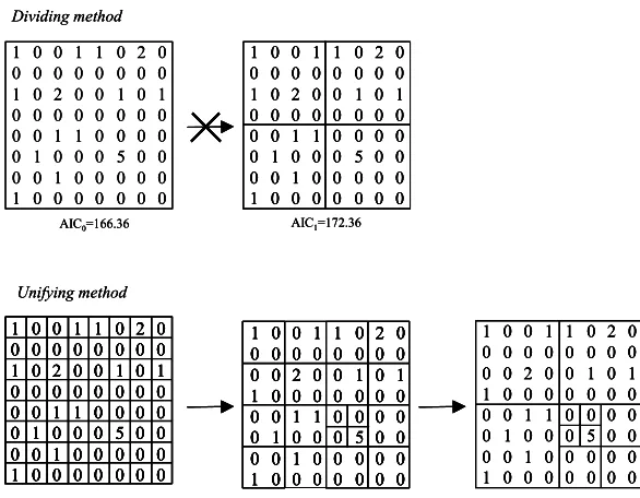
That is, by comparing equation (3) with equation (4), we can say that a model with a small value is adequate when considering the trade-off relationships between amount of information and amount of data. If AIC0 is less than AIC1, the sub-area should form the larger sub-area whose size is 2k+1. On the contrary, if AIC0 is greater than AIC1, a larger sub-area should not be formed and we should adopt the smaller sub-area whose size is 2k as the adequate space-cluster. Furthermore, by referring to formula (2), we obtain the following equations when the attribute value is defined as a continuous value. We can then evaluate space-clusters using this equation as follows:

(

log2 log ˆ 1

)

2(1 1)

2

AIC 2( 1) 2

0 = +

π

+

σ

+ + +

k _, ₍₅₎

where

   

 

−

= +

∈

+

∑

2( 1) 2 2 ) 1 ( 2 2

2 2

1

ˆ _k

C i i k

C x

σ

(

log2 log ˆ 1

)

2(4 1)

2

AIC 2( 1) 2

1= k+

π

+

σ

+ + + (6)

where

   

 

−

=

∑ ∑

∑

= = ∈ +

4

1 2

2 4

1 2 )

1 ( 2 2

2 2

1 ˆ

l k l l ic

i k

c x

l σ

However, _log

_σ

_ˆ2_{in equation (6) cannot be estimated at the time of}_k_{=0 (namely, in case of the}

smallest unit cell). Therefore, when the attribute value is defined as a continuous value, the sub-area formed of the four smallest unit cells can be the smallest space-cluster.

3.2 Comparison of Methods: "Dividing" and "Unifying"

(10)

5 2 0 1 0 1 0 2 0 0 1 1 0 1 0 0 0 0 0 0 0 0 0 0 0 0 0 1 0 1

0 0 0 0 0 0 0 0 1 1 0 0 0 0 0 1 0 0 0 0 0 0 0 0 0 0 0 1 0 0 0 0 0 0 5 2 0 1 0 0 0 2 0 0 1 1 0 1 0 0 0 0 0 0 0 0 0 1 0 0 0 1 0 1

0 0 0 0 0 0 0 0 1 1 0 0 0 0 0 1 0 0 0 0 0 0 0 0 0 0 0 1 0 0 0 0 0 0

5 2

0

1 0

1 2 0

0 0 1 1 0 1 0 0 0 0 0 0 0 0 0 0 0 0 0 1 0 1

0 0 0 0 0 0 0 0 1 1 0 0 0 0 0 1 0 0 0 0 0 0 0 0 0 0 0 1 0 0 0 0 0 0 Unifying method

AIC1=172.36

AIC0=166.36 5 2 0 1 0 0 0 2 0 0 1 1 0 1 0 0 0 0 0 0 0 0 0 1 0 0 0 1 0 1

0 0 0 0 0 0 0 0 1 1 0 0 0 0 0 1 0 0 0 0 0 0 0 0 0 0 0 1 0 0 0 0 0 0

5 2 0 1 0 0 0 2 0 0 1 1 0 1 0 0 0 0 0 0 0 0 0 1 0 0 0 1 0 1

0 0 0 0 0 0 0 0 1 1 0 0 0 0 0 1 0 0 0 0 0 0 0 0 0 0 0 1 0 0 0 0 0 0 Dividing method 5 2 0 1 0 1 0 2 0 0 1 1 0 1 0 0 0 0 0 0 0 0 0 0 0 0 0 1 0 1

0 0 0 0 0 0 0 0 1 1 0 0 0 0 0 1 0 0 0 0 0 0 0 0 0 0 0 1 0 0 0 0 0 0 5 2 0 1 0 0 0 2 0 0 1 1 0 1 0 0 0 0 0 0 0 0 0 1 0 0 0 1 0 1

0 0 0 0 0 0 0 0 1 1 0 0 0 0 0 1 0 0 0 0 0 0 0 0 0 0 0 1 0 0 0 0 0 0

5 2

0

1 0

1 2 0

0 0 1 1 0 1 0 0 0 0 0 0 0 0 0 0 0 0 0 1 0 1

0 0 0 0 0 0 0 0 1 1 0 0 0 0 0 1 0 0 0 0 0 0 0 0 0 0 0 1 0 0 0 0 0 0 Unifying method 5 2 0 1 0 1 0 2 0 0 1 1 0 1 0 0 0 0 0 0 0 0 0 0 0 0 0 1 0 1

0 0 0 0 0 0 0 0 1 1 0 0 0 0 0 1 0 0 0 0 0 0 0 0 0 0 0 1 0 0 0 0 0 0 5 2 0 1 0 0 0 2 0 0 1 1 0 1 0 0 0 0 0 0 0 0 0 1 0 0 0 1 0 1

0 0 0 0 0 0 0 0 1 1 0 0 0 0 0 1 0 0 0 0 0 0 0 0 0 0 0 1 0 0 0 0 0 0

5 2

0

1 0

1 2 0

0 0 1 1 0 1 0 0 0 0 0 0 0 0 0 0 0 0 0 1 0 1

0 0 0 0 0 0 0 0 1 1 0 0 0 0 0 1 0 0 0 0 0 0 0 0 0 0 0 1 0 0 0 0 0 0

5 2 0 1 0 1 0 2 0 0 1 1 0 1 0 0 0 0 0 0 0 0 0 0 0 0 0 1 0 1

0 0 0 0 0 0 0 0 1 1 0 0 0 0 0 1 0 0 0 0 0 0 0 0 0 0 0 1 0 0 0 0 0 0 5 2 0 1 0 0 0 2 0 0 1 1 0 1 0 0 0 0 0 0 0 0 0 1 0 0 0 1 0 1

0 0 0 0 0 0 0 0 1 1 0 0 0 0 0 1 0 0 0 0 0 0 0 0 0 0 0 1 0 0 0 0 0 0

5 2 0 1 0 0 0 2 0 0 1 1 0 1 0 0 0 0 0 0 0 0 0 1 0 0 0 1 0 1

0 0 0 0 0 0 0 0 1 1 0 0 0 0 0 1 0 0 0 0 0 0 0 0 0 0 0 1 0 0 0 0 0 0

5 2 0 1 0 0 0 2 0 0 1 1 0 1 0 0 0 0 0 0 0 0 0 1 0 0 0 1 0 1

0 0 0 0 0 0 0 0 1 1 0 0 0 0 0 1 0 0 0 0 0 0 0 0 0 0 0 1 0 0 0 0 0 0

5 2

0

1 0

1 2 0

0 0 1 1 0 1 0 0 0 0 0 0 0 0 0 0 0 0 0 1 0 1

0 0 0 0 0 0 0 0 1 1 0 0 0 0 0 1 0 0 0 0 0 0 0 0 0 0 0 1 0 0 0 0 0 0

5 2

0

1 0

1 2 0

0 0 1 1 0 1 0 0 0 0 0 0 0 0 0 0 0 0 0 1 0 1

0 0 0 0 0 0 0 0 1 1 0 0 0 0 0 1 0 0 0 0 0 0 0 0 0 0 0 1 0 0 0 0 0 0

5 2

0

1 0

1 2 0

0 0 1 1 0 1 0 0 0 0 0 0 0 0 0 0 0 0 0 1 0 1

0 0 0 0 0 0 0 0 1 1 0 0 0 0 0 1 0 0 0 0 0 0 0 0 0 0 0 1 0 0 0 0 0 0 Unifying method

AIC1=172.36

AIC0=166.36 5 2 0 1 0 0 0 2 0 0 1 1 0 1 0 0 0 0 0 0 0 0 0 1 0 0 0 1 0 1

0 0 0 0 0 0 0 0 1 1 0 0 0 0 0 1 0 0 0 0 0 0 0 0 0 0 0 1 0 0 0 0 0 0

5 2 0 1 0 0 0 2 0 0 1 1 0 1 0 0 0 0 0 0 0 0 0 1 0 0 0 1 0 1

0 0 0 0 0 0 0 0 1 1 0 0 0 0 0 1 0 0 0 0 0 0 0 0 0 0 0 1 0 0 0 0 0 0 Dividing method

AIC1=172.36

AIC0=166.36 5 2 0 1 0 0 0 2 0 0 1 1 0 1 0 0 0 0 0 0 0 0 0 1 0 0 0 1 0 1

0 0 0 0 0 0 0 0 1 1 0 0 0 0 0 1 0 0 0 0 0 0 0 0 0 0 0 1 0 0 0 0 0 0

5 2 0 1 0 0 0 2 0 0 1 1 0 1 0 0 0 0 0 0 0 0 0 1 0 0 0 1 0 1

0 0 0 0 0 0 0 0 1 1 0 0 0 0 0 1 0 0 0 0 0 0 0 0 0 0 0 1 0 0 0 0 0 0

5 2 0 1 0 0 0 2 0 0 1 1 0 1 0 0 0 0 0 0 0 0 0 1 0 0 0 1 0 1

0 0 0 0 0 0 0 0 1 1 0 0 0 0 0 1 0 0 0 0 0 0 0 0 0 0 0 1 0 0 0 0 0 0 Dividing method

Figure 4: Comparison of dividing method and unifying method

3.3 Application to Actual Spatial Data

(11)

Ra tio of f em al e-w or ke rs( % )

Original data Optimal space-cluster

200 100 0 300 30 40 50 60 70

100 200 300

0 30 40 50 60 70 300 200 100 0 30 40 50 60 70 80 90 300 200 100 0 30 40 50 60 70 80 90 R at

io of nu

cl ear fa m il y(%) 300 200 100 0 0 10 20 30 300 200 100 0 0 10 20 30 300 200 100 0 0 100 200 300 400 500 300 200 100 0 0 100 200 300 400 500 T he num be r of fish er m an T he num be r of m er cha nt s

Figure of Data-Distribution Optimal space-cluster Ra tio of f em al e-w or ke rs( % )

Original data Optimal space-cluster

200 100 0 300 30 40 50 60 70 200 100 0 300 30 40 50 60 70

100 200 300

0 30 40 50 60 70

100 200 300

0 30 40 50 60 70 300 200 100 0 30 40 50 60 70 80 90 300 200 100 0 30 40 50 60 70 80 90 300 200 100 0 30 40 50 60 70 80 90 300 200 100 0 30 40 50 60 70 80 90 R at

io of nu

cl ear fa m il y(%) 300 200 100 0 0 10 20 30 300 200 100 0 0 10 20 30 300 200 100 0 0 10 20 30 300 200 100 0 0 10 20 30 300 200 100 0 0 100 200 300 400 500 300 200 100 0 0 100 200 300 400 500 300 200 100 0 0 100 200 300 400 500 300 200 100 0 0 100 200 300 400 500 T he num be r of fish er m an T he num be r of m er cha nt s

Figure of Data-Distribution Optimal

space-cluster

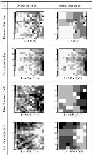
Figure 5: Optimal Space-cluster and Data Distribution

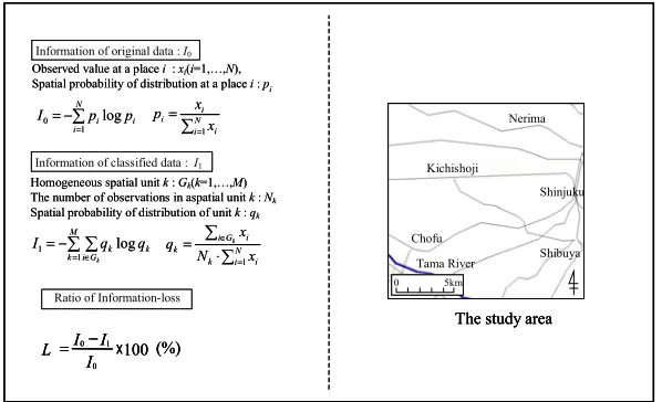
4. Visualization of Space-Cluster

(12)

information loss defined in figure 6 is also shown. The figure 7 shows clearly that if we create the appropriate space-cluster, the space distribution characteristic of the original data can be grasped more easily. The correct results are obtained both in cases where the data is defined as a continuous value and as a discrete value. However, it is necessary to pay attention to the information loss increasing slightly.

Shinjuku Kichishoji

Chofu

5km 0

Nerima

Shibuya Tama River

The study area

Ratio of Information-loss

∑ =

− = N

i i i p p I

1

0 log _∑

=

= N i i

i

i _x

x p

1

∑ ∑ = ∈

− = M

k iGk k k q q I

1

1 log _∑

∑ = ∈

⋅

= _N

i i k

G i i

k _N _x

x

q k

1

Observed value at a place i:xi(i=1,…,N),

Spatial probability of distribution at a place i: pi

Homogeneous spatial unit k: Gk(k=1,…,M)

The number of observations in aspatial unit k: Nk

Spatial probability of distribution of unit k: qk

Information of original data : I0

Information of classified data : I1

(%) 100

0 1 0−

=

I I I L

Shinjuku Kichishoji

Chofu

5km 0

Nerima

Shibuya Tama River

The study area

Shinjuku Kichishoji

Chofu

5km

0 5km

0

Nerima

Shibuya Tama River

The study area

Ratio of Information-loss

∑ =

− = N

i i i p p I

1

0 log _∑

=

= N i i

i

i _x

x p

1

∑ ∑ = ∈

− = M

k iGk k k q q I

1

1 log _∑

∑ = ∈

⋅

= _N

i i k

G i i

k _N _x

x

q k

1

Observed value at a place i:xi(i=1,…,N),

Spatial probability of distribution at a place i: pi

Homogeneous spatial unit k: Gk(k=1,…,M)

The number of observations in aspatial unit k: Nk

Spatial probability of distribution of unit k: qk

Information of original data : I0

Information of classified data : I1

(%) 100

0 1 0−

=

I I I

L 100(%)

0 1 0−

=

I I I L

(13)

Original smallest cell Optimal Space-cluster

31

8

3

1

0 0

L = 0.32 (%)

31

8

3

1

0.39

0

L = 7.51 (%)

51.9

49.8

47.3

45.0

0 40.0

L = 3.12 10-2_(%) 64.1

50.7

47.3

44.4

0 40.9

L = 0.57 10-2_(%)

0 43.0 49.7 56.5 65.1 85.4

L = 1.87 10-2_(%) 0 42.1 48.3 51.9 59.9 73.1

L = 12.04 10-2_(%) 0

25 63 138 256 459

L = 6.60 10-1_(%) 0 26 63 138 256 459

L = 6.96 10-1_(%)

R

at

io of

fe

m

al

e-w

or

ke

rs

(%

)

R

at

io

of

nu

cl

ea

r f

am

ily

(%

)

T

he n

um

ber

o

f f

is

her

m

an

T

he

n

umb

er

o

f me

rc

ha

nt

s

(14)

5. Summery and conclusions

The method of obtaining the space-cluster based on the evaluation function of AIC is proposed, with consideration to the distribution characteristic of spatial data. Moreover, the appropriate space-cluster is visualized by the information loss minimization method. Using the proposed method, the information contained in the original spatial data can be visualized, and we can grasp and understand the statistical characteristics of geographical data.

6. Acknowledgements

The author would like to express his thanks for the valuable comments from Mr. Paul Torrens, Centre for Advanced Spatial Analysis, University College London. Also, the author would like to give his special thanks to Mr. Hiroki Yamanaka, Graduate Student of Tokyo Institute of Technology, for computer-based numerical calculations.

References

Akaike H, 1972, “Information theory and an extension of the maximum likelihood principle” Proceedings of the 2nd_{International Symposium on Information Theory Eds B N Petron, F Csak} (Akademiai kaido, Budapest), pp. 267-281.

Akaike H, 1974, “A new look at the statistical model identification” IEEE Transactions on Automatic Control AC19, pp.716-723.

Anselin L, 1995, “Local Indicator of Spatial Association - LISA”, Geographical Analysis Vol.27, No.2, pp.93-115.

Batty M, 1974, “Spatial Entropy”, Geographical Analysis, Vol.6, pp.1-31.

Batty M, 1976, “Entropy in Spatial Aggregation”, Geographical Analysis, Vol.8, pp.1-21.

Batty M, 1978, “Speculations on an information theoretic approach to spatial representation”, in Studies in Applied Regional Science 10: Spatial Representation and Spatial Interaction, Edt I Masser, P Brown (Martinus Nijhoff, Leiden, The Netherlands), pp.115-147.

Civco D L, 1993, “Artificial neural networks for land-cover classification and mapping”, Int. J. Geographical Information Systems, Vol.7, No.2, pp173-186.

Fotheringham A S and Wong D W S. 1991, “The modifiable areal unit problem in multivariate statistical analysis”, Environmen and Planning A, Vol.23, pp.1025-1044.

(15)

Li-Xia, 1996, “A method to improve classification with shape information”, International Journal of Remote Sensing Vol.17, No.8, pp.1473-1481.

Liebetrau A M and Rothman E D, 1977, “A classification of spatial distributions based upon several cell sizes”, Geographical Analysis, Vol.9, pp.14-28.

Margules C R, Faith D P and Belbin L, 1985, “An adjacency constraint in agglomerative hierarchical classifications of geographic data”, Environment and Planning A, Vol.17, pp.397-412.

Nakaya T. 2000, “An information statistical approach to the modifiable areal unit problem in incidence rate maps”, Environment and Planning A, Vol.32, pp.91-109.

Openshaw S, 1977, “Optimal zoning systems for spatial interaction models”, Environment and Planning A, Vol.9, pp.169-184.

Osaragi T, 2001, “Classification method of spatial data and its information loss”, Working Paper at CASA, University College London.

Roy J R, Batten D F and Lesse P F, 1982, “Minimizing information loss in simple aggregation”, Environment and Planning A, Vol.14, pp.973-980.

Tamagawa H, 1987, “A study on the optimum mesh size in view of the homogeneity of land use ratio”, Papers on City Planning Vol.22, pp.229-234. (in Japanese)

Higuchi T, Tamagawa H and Ishak A B P, 1988, “A study on the optimum mesh size for continuous variables – An example by using a mental map –“, Papers on City Planning Vol.23, pp.37-42. (in Japanese)