Phase extraction in dynamic speckle interferometry:
proposal of a road map
S. Equisa, and P. Jacquot
EPFL, Nanophotonics and Metrology Laboratory, Station 11, CH-1015 Lausanne, Switzerland
Abstract. Of all the two-beam interference patterns, the ones obtained in speckle interferometry (SI) are the most difficult to be phase-demodulated. Many solutions exist in classical smooth-wave interferometry and alike techniques, both in static and dynamic regimes. In SI, the three constituents of the signals – the background, the modulation and the phase – are all basically random variables. There is no way to make a prediction of the evolution of these variables outside the small size of the correlation volumes – the volumes defined by the average speckle grain. To some extent, the classical methods can be adapted to SI. Here, we prefer to develop a series of new processing tools tailored to the specificities of the dynamic SI signals: the cooperative use of the empirical mode decomposition (EMD), the Hilbert transform (HT), and the three dimensional piecewise processing (3DPP) for recovering efficiently the phase of these signals.
1 Introduction
During the elapsed decade, photomechanics has established itself as a prominent discipline of experimental mechanics. It consists essentially in integrating simulations and experimentation for validation, generalization and optimization purposes – the experiments being carried out by means of full-field optical measurements methods. The most relevant methods are, by far, DIC and SI. DIC stands for “digital image correlation” and SI for “speckle interferometry”. The impact of both types of methods strongly depends on the ability to process the rough acquired data, i.e. to convert intensity images and fringe patterns into sets of mechanically interesting variables. This article proposes a complete solution of this problem in the case of SI applied to the analysis of the deformation of solid bodies subjected to dynamic loadings.
The next section is a short reminder about the available methods mostly developed for processing smooth interference signals. It serves to highlight the limits of these methods when confronted to non-stationary SI signals. The core of the article is then devoted to describe three processing tools, completely independent in their modi operandi, but specifically conceived for SI signals and suggested to be used all three together cooperatively. The first tool is a pre-processing means to eliminate the varying intensity background of the signals. It relies on a technique fully tried and tested in other domains, but never in SI: the empirical mode decomposition (EMD). With a centred signal, the task is easier and it becomes sound to look at standard procedures for inverting a cosine function: our second tool is quite naturally the most often used quadrature operator, namely the
a
e-mail : [email protected]
Hilbert transform (HT). The inevitable existence of parts of the SI signals exhibiting nearly zero modulations calls for a last treatment: the three dimensional piecewise processing (3DPP). In our context, 3D means two spatial and one temporal coordinates, and though all the processing is first done in 1D along the time axis, the ultimate goal is obviously to create movies showing the deformation behaviour of the full object surface. In 3D, the signals intervals below a predefined modulation threshold are purely and simply discarded. The missing parts are refurbished by an ad hoc interpolation procedure using only the most reliable and closest preserved data. This is made possible thanks to the properties of the Delaunay triangulation (DT).
The last section presents a complete example of the joint utilization of these three processing tools and summarizes their main features.
2 Strengths and weaknesses of phase extraction methods
2.1 Extracting the phase of interferometric signals
The intensity IR of a two-beam interference pattern invariably reads:
1 2 2 1 2 R
I I I I I JcosM
,
(1)where I1 and I2 are the intensities of the two waves, M their phase difference, J the normalized module of the cross-correlation of the two amplitudes. SI arrangements are operated with lasers of long coherence lengths, so that J is taken equal to 1 in the rest of the paper. The arguments of the functions, specifying when and where the signal is observed, are omitted for simplicity. Note however that a megapixel camera operating at 100 Hz is able to record during one second 108 independent values of the interferometric signal, equivalent of what would be obtained by 106 punctual sensors in parallel, read out one hundred times a second. Note also that the size of the corresponding data files amounts to 1Gbit if the intensities are digitized to 10 bits. The phase is proportional to the optical path difference between the two waves and thus encodes the quantity of interest. This path difference is naturally measured in unit of the wavelength of the light, whence the sub-micrometric interferometric sensitivity. The exact relationship between M and the investigated physical quantity is beyond the scope of the present investigation. SI aims to render this relationship as simple and univocal as possible, by making M proportional to a particular projection of the displacement vector or to its partial derivatives, depending on the chosen geometry of the optical arrangement, [1-3]. In regard of sensitivity, density of interrogated points, flexibility in the choice of the measurand and capacity of real time visualization, interferometry is overwhelmingly preferred to image correlation. In order to comprehend better what the processing of interferometric signals means, Eq. (1) can be rewritten as:
2 ;
R
I BM cosM M dB
,
(2)where B is the background or arithmetic mean of the intensities of the two interfering light fields, and M represents the modulation or geometric mean of these two intensities – 4M being the difference between two consecutive maximum-minimum. The processing consists in solving the above equation for M, from the knowledge of the resultant intensity, IR, also called specklegram in SI, and using appropriate strategies either to compute or to eliminate the unknowns B and M.
2.2 Available methods
necessarily universally accepted, but are all recognized by the search engines of the bibliographic source indexes and give an easy access to the corresponding literature.
Fig. 1. Principal categories of phase extraction methods.
The utilization rate of these methods in actual experiments is difficult to evaluate. The choice of a method depends on many factors and, at the first rank, on the nature smooth or speckled of the interfering waves. Without paying to much attention to the details, morphology and definite transforms are best adapted to the processing of dynamic fringe patterns obtained with smooth waves: classical interferometry, photoelasticimetry, fringe projection. Phase-shifting is by far the choicest method for static or slow deformation regimes, when there is enough time to prepare several phase-shifted versions of the same interference state. As yet, stochastic methods, though promising, have not reached a wide acceptance and suffer from a lack of precise characterization in practical conditions. SI introduces particular requirements as discussed in the next section.
2.3 The status of SI
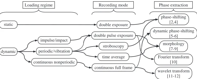
In SI, owing to the fundamental random nature of speckle waves, B and M are not only unknown, but also highly spatially and temporally fluctuating quantities. The volumes inside which it is reasonable to make inter- and extrapolation calculations are as small as the average size of isolated speckle grains, i.e. of the order of 3x3x100 Pm3 for visible wavelengths and usual apertures [1-3]. The speckle fluctuations, the existence of phase uncertainties or singularities, the linearity and non-stationary behaviour of Eq. (2), the high dimensionality in dynamic regimes, not to mention different types of noise corrupting the signals, make difficult the computation of the phase M. Figure 2 summarizes the possible choices of a processing method in SI and orients toward a few pertinent references. Still a number of methods are available. However, there are large differences in their frequency of utilization, and the cases of impulse and continuous non-periodic loadings, incompletely solved, remain an issue.
Fig. 2. Available processing methods in SI with respect to the loading regime and the recording mode.
Morphology Fringe tracking
Regularization Spline fitting
Definite transforms Fourier Stochastic methods Hilbert
Wavelets
Particle filter Kalman filter
Spectral estimation Phase probing Heterodyning
Phase-shifting
PLL (Phase Lock Loop)
Loading regime Recording mode Phase extraction
static
dynamic
impulse/impact
periodic/vibration
continuous nonperiodic
double exposure
double pulse exposure
stroboscopy
time average
continuous full frame
phase-shifting [2,4]
morphology [7-9] Fourier transform
[10]
dynamic phase-shifting [5-6]
Considering that dynamic regimes are the more frequent and that processing schemes in this case are the most open to improvements, we focused our developments on the processing of long sequences of recorded specklegrams, obtained in continuous non-periodic loading regimes.
2.4 Proposed road map for extracting the phase of dynamic SI signals
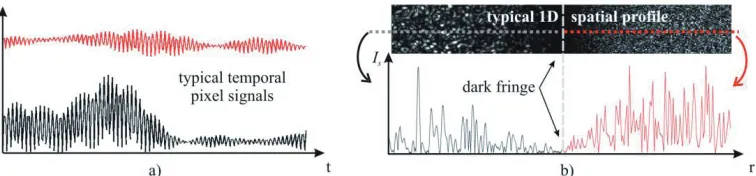
In SI, two broad categories of signals should be distinguished, due to their peculiar appearance and features: the signals given by each pixel along the temporal axis, and those resulting from any 1D spatial cut made in the correlation fringes, i.e. the pattern obtained by the absolute subtraction, or similar arithmetic operations, of two correlated specklegrams associated to two states of the object deformation. Figure 3, directly drawn from Eq. (1) or (2) valued with arguments of an experimental or a simulation nature, highlights the obvious differences between the two types of signals, which portray all the known situations in SI: the cases of spatially resolved or unresolved recordings, and the introduction or not of a carrier signal. Incidentally, it is worth noting that Figure 3 a) represents also the case of a 1D spatial profile of correlation fringes in the spatially resolved regime, with a spatial carrier and in a direction orthogonal to the carrier fringes.
Fig. 3. Typical appearance of SI signals; a) temporal pixel signal in the spatially resolved (black) and unresolved (red) cases; b) 1D spatial cut in the plane of the correlation fringes in the same cases. In terms of signal processing, it is much more appealing to attempt to treat the signals on the left side of the figure than on the right. For these latter, the horizon appears limited to strategies involving the smoothing of the fluctuations by low pass filtering, resulting inevitably in a reduction of the spatial resolution. On the contrary, signals of the left types exist in many domains and have received much more attention from the signal processing community. A vast set of methods is available on a self-service basis. We chose to treat temporal pixel signals. The general trend is to eliminate the varying background, and hence to further demodulate a centred signal, again in both cases with many existing ways of performing the corresponding computations. Our approach is to advocate the use of the empirical mode decomposition (EMD) followed by a Hilbert transform (HT) for the first two tasks. We add a third processing step, specific to SI signals, meant for solving the problem of the under-modulated parts of the signals: the three dimensional piecewise processing (3DPP). Each of the three procedures is now reviewed in the forthcoming sections.
3 A useful pre-processing tool: the Empirical Mode Decomposition
3.1 The EMD: an adaptive technique for background removal in SI
but with self-adaptive band-filters. By construction, the IMFs have a well-behaved HT, and more generally allow good phase extraction. An extensive description of the EMD and the HT is given in [13-15]. In the context of dynamic SI, we conceived a dedicated algorithm: it extracts the interference term (2McosM in Eq.2) as the first IMF of the decomposition in a single iteration. The algorithm removes the mean envelope – very close to the true background intensity (2B in Eq.2) – computed from a cubic-spline fitting of the raw signal extrema (the cubic-spline kernel is acknowledged to best perform in most cases). Figure 4 illustrates this functioning on simulated signals.
Fig. 4. a) Non-stationary signal with upper, lower and mean envelopes, and b) EMD-centred signal.
3.2 What makes the EMD a highly valuable pre-processing tool in SI?
The outcome of the EMD algorithm is actually multiple. In addition of the centered signal on which phase computation can be carried out, the location of the signal extrema provides a rough estimation of the instantaneous frequency (IF) - rather the mean of the IF over every half-period. This estimation is very sensitive to the quantization noise, due the fact that true extrema are unlikely located at sampling points, but is helpful notably for a rough evaluation of the phase in long experiments. Moreover, the envelopes computation gives also the modulation depth which is helpful to appraise the reliability of the phase computation, as it will be seen farther, and which can also be of use to phase tracking techniques (for instance normalizing the gain of a Digital Phase Lock Loop).
3.3 On the complexity of the EMD
The temporal approach has proven to be suited for dynamic experiments characterization [11, 13], as it allows to get rid of the correlation length limitation, and to probe the surface at will. It is however at the expense of data manipulation prior to the actual phase extraction. The procedure needs to rearrange a 3D matrix (the two space coordinates of the sensor and one temporal coordinate) into a set of one-dimensional signals. Considering a matrix containing Nx×Ny×Nt elements, the operation complexity is O(N3), even if the operation mainly involves memory allocation and is thus rather greedy in memory space than in processor resources. Moreover, a great amount of reading and writing operations can be saved if the Nx×Ny temporal signals are gathered in stacks (Nx stacks of Ny signals for example). The EMD algorithm involves itself pretty simple operations and its complexity can be estimated to be asymptotically O(Nt). For example, the processing of a stack of 1000 signals of 1024 time samples each takes less than 1 s for the re-allocation, 30 s for EMD itself, and 5 s more for the HT-based phase computation, on a common computer equipped with a Core2 2.66 GHz processor.
4 Actual phase extraction using the Hilbert transform
pure phase filter in the reciprocal space, adding S/2 to the phase of positive frequencies components and -S/2 to the phase of the negative ones, while leaving the amplitudes unimpaired:
( ), 0
( )
( ), 0
iS for
FT HT s t
iS for
Q Q
Q Q
!
ª º ®
¬ ¼ ¯ , (3)
where Q is the Fourier domain coordinate and S(Q) is the FT of s(t). The phase is eventually computed from the complex-valued signal with the arctan function in the range ]-S, S].
5. Three dimensional piecewise processing
–
3DPP
5.1 Dealing with ill-modulated signals in SI: a topical issue and a proposed solution
Due to the intrinsic randomness of the intensity and the phase of a speckle field, the temporal SI signal will experience strong fluctuations of modulation and local mean, making tricky and prone to errors any phase extraction procedure. In the vicinity of areas of null modulation, noise due to the electronic chain of acquisition, or to laser power fluctuations, or also to mechanical disturbances becomes preeminent. In addition, it is well-known, that the lower the modulation, the higher the random phase errors induced by decorrelations. Due to the 1D unwrapping operation, the error will propagate and corrupt the whole phase dataset. Several strategies aiming at reducing or eliminating the phase errors are available, ranging from decorrelations compensation by appropriate adjustments of the setup, to specific filtering procedures, where the kernel coefficients depend on the confidence levels of the measurements. Pixel weights proportional to the square of the modulation represent theoretically an ideal choice. Filtering however always dilutes and spreads to some extent the errors over larger areas, and can even fail when the kernels happen to contain invalid data only. The 3DPP is meant for avoiding such shortcomings.
The 3DPP method consists in discarding, purely and simply, the regions, within each temporal pixel history, where the modulation is lower than a predefined threshold [13, 17]. The so-built regions of missing data, of random length and location, are filled by the information carried by reliable well-modulated neighboring pixels, using an interpolation procedure based on the so-called Delaunay triangulation DT. This triangulation is constructed inside the convex hull of the data set. The convex hull in 2D might be seen as a rubber band surrounding a set of nails driven in a wooden board, the latter ones representing our mesh of valid data. It does not guarantee a constant definition of the boundaries of the area of interest (AOI). It is thus mandatory to have at each instant fixed points on which the convex hull will be constructed. To do so, we simply make sure that the AOI is always surrounded by pixels, naturally or artificially, labelled as valid with values of IF, either imposed by a priori knowledge, by averaging or fitting the values of the AOI border. It is actually desirable to build a triangulation which minimizes the size of the facets. Indeed, it sounds natural to expect from the triangulation-interpolation process that each interpolated point is computed by relying on the closest data. The DT actually fulfils this criterion by generating the least stretched facets and thus preserves at best the spatial resolution.
5.2 On the implementation of the 3DPP procedure, and its complexity
At one instant k, the 3DPP technique is composed of three main steps. The first one is the binary classification of the data, which consists in a basic test over the Nx×Ny pixels. Given a certain threshold, the Nx×Ny values of modulation are compared to this threshold and a value 0 or 1 is then attributed to the pixel. This operation complexity is quadratic, i.e. O(N2).
sampled on a regular grid. A trade-off must be found between noise removal, spatial resolution and computation load. A too low threshold will not discard regions of pixel signals with poor modulation intensity prone to the highest phase error. Conversely, a too high threshold will lead to a very discriminate test and the triangulation-interpolation step will rely on very few points, inducing a great loss of spatial resolution, with no significant improvement of the quality of the result. As an example, the processing of a batch of 1024 frames of 200×200 pixels lasts 20 minutes for a threshold which yields the best compromise between spatial resolution preserving and noise removing (49% of discarded pixels), on a common computer equipped with a Core2 2.66 GHz processor.
6. Results and outlook
6.1 Assessment of the EMD/HT/3DPP method
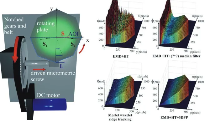
In a SI setup with in-plane sensitivity (Leendertz configuration), the object is illuminated by two divergent laser beams of equal intensity, whose directions are designated by the unit vectors S1 and S2 in Figure 5. The observation direction coincides with the object surface normal and the sensitivity is equal to 8.7 rad/Pm. In this experiment, no optical temporal carrier has been introduced – mandatory to find out the direction of the deformation in order to have the largest measurement bandwidth, which otherwise would have to be shared with the carrier frequency, and to assess the method with a very wide range of deformation rates. It is thus enough to process the temporal pixels of half the plate. The phase maps obtained after a maximum displacement of 59 Pm (i.e. about 514 radians) are shown in the right part of Figure 5. The phase extraction is severely polluted for pixels experiencing less and less fringes of displacement (toward the central part of the plate). The median filter, acknowledged to be edge-preserving and efficient with random salt-pepper noise, with a fixed kernel size, fails in the central part of the plate whatever the chosen weights. The Morlet wavelet ridge tracking algorithm [11] is well-known to be particularly robust and efficient, but encounters difficulties to converge when a large range of IF is considered. The benefit of the 3DPP procedure appears finally in an obvious manner, with a high reliability and a clear definition of the edges, thanks to a proper definition of the convex hull.
6.2 Outlook
The rigid body rotation experiment has been carried out to assess the proposed processing scheme. It features indeed a broad range of IF so as to point out the self-adaptability of both EMD and 3DPP and the noise removal power of this latter tool. These tools have been used also to characterize more complex behaviors, like the in-plane compression of a piece of rubber [13], the propagation of heat in water and the blending of liquids with different refraction indexes: they have proved to be very efficient and versatile for SI temporal signals, even beyond the classical correlation length limit. It is worth emphasizing again the fact that the EMD and the 3DPP techniques, respectively prior and subsequent steps to phase computation, are completely independent. The outcome of the first one is a centered signal with the ad-hoc shape for phase determination, while the second one, when fed with IF and modulation maps, yields smooth phase maps built on the most reliable data.
The world of stochastic methods for frequency estimation and tracking is very rich and promising but needs a pre-processing tool to be able to cope with the peculiarities of SI signals. Thanks to the EMD, this bench of methods becomes within reach. It can definitely help to conceive accurate, fast phase computation methods with an even better noise immunity than the HT-based phase computation.
Finally, our answer to the under-modulation issue showed some good behavior in low SNR regions. Some improvements can be done to be able to treat the case of objects with non-convex shapes, and the case of spatial discontinuities as well. Another point that would deserve to be pursued is the surface tiling to lighten the computation burden. A tiling depending on the activity with criteria derived from the temporal and spatial phase gradients would permit to process the pixels, sparsely spread over the surface, which are the most relevant to treat (around a crack, in a high spatial displacement gradient area, and so on...).
Acknowledgments
This work is supported by the Swiss National Science Foundation.
References
1. A. E. Ennos, Speckle interferometry, Laser Speckle and Related Phenomena, (Springer Verlag, Berlin, 1984)
2. K. Creath, Appl. Opt., 24, 3053-3058, (1985) 3. P. Jacquot, Strain, 44, 57-69, (2008)
4. J.M. Huntley, Appl. Opt. 32, 3047-3052, (1993)
5. X. Colonna de Lega, P. Jacquot, Appl. Opt., 35, 5115-5121, (1996) 6. T.E. Carlsson, A. Wei, Appl. Opt., 39, 2628-2637, (2000)
7. E. Robin, V. Valle, and F. Bremand, Appl. Opt., 44, 7261-7269, (2005)
8. M. Servin, J.L. Marroquin, and J.A. Quiroga, J. Opt. Soc. Am. A, 21, 411-419, (2004) 9. L. Bruno, Opt. Express, 15, 4835-4847, (2007)
10. M. Takeda, H. Ina, and S. Kobayashi, J. Opt. Soc. Am., 72, 156-160, (1982) 11. X. Colonna de Lega, EPFL thesis n° 1666, Lausanne, (1997)
12. Y. Fu, Appl. Opt., 44, 959-965, (2005)
13. S. Equis, EPFL thesis n° 4514, Lausanne, (2009) 14. S. Equis and P. Jacquot, Strain, (2008)
15. S. Equis and P. Jacquot, Opt. Express, 17, 611–23, (2009)