A Low Complexity Direction of Arrival Estimation Algorithm by Reinvestigating the Sparse Structure of Uniform Linear Arrays

A Low Complexity Direction of Arrival Estimation Algorithm by

Reinvestigating the Sparse Structure of Uniform Linear Arrays

Fenggang Sun1, 2, Peng Lan1, *, Bin Gao2, and Lizhen Chen1

Abstract—In this paper, we present a new computationally efficient method for direction-of-arrival (DOA) estimation in uniform linear arrays (ULAs). A sparse uniform linear array (SULA) structure is firstly extracted from the conventional ULA to exploit its advantage in high resolution. By performing the multiple signal classification (MUSIC), the noise subspace of the SULA is simultaneously orthogonal to the steering vectors corresponding to the true DOAs and several virtual DOAs, where all the true and virtual DOAs for each source are uniformly distributed in the sine domain. Then we divide the total angular field into several small sectors and search over an arbitrary sector. Finally, the true DOAs can be distinguished by the noise subspace of the original ULA. Since the proposed method involves a limited spectral search and a reduced-dimension noise subspace, hence it is quite computationally efficient. Simulation results are provided to verify the effectiveness of the proposed method in terms of computational complexity, estimation accuracy, and resolution performance.

1. INTRODUCTION

In array signal processing, direction-of-arrival (DOA) estimation is of practical interest in radar, sonar, wireless communications and other applications [1, 2]. Over the past decades, various methods have been developed to estimate DOAs, including Capon [3], multiple signal classification (MUSIC) [4], root-MUSIC [5], and estimation of signal parameters via rotational invariance techniques (ESPRIT) [6]. Among these methods, the MUSIC method can offer a reasonable resolution and can be easily applied in arbitrary array without dependence on array configuration. Therefore it is regarded as one of the most popular techniques. However, since the MUSIC method involves a computationally demanding burden, its utilization can be prohibitively expensive especially when real-time processing is required.

For the conventional MUSIC method, the computational complexity is mainly caused by two steps, i.e., subspace decomposition and spectral search. Efficient methods have been proposed to reduce the complexity of subspace decomposition [7, 8]. The fast subspace decomposition (FSD) technique in [7] can reduce the computation to O(M2K), whereM and K are the numbers of sensor elements and sources, respectively. In [8], a novel real-valued MUSIC estimator with only real-valued subspace decomposition is proposed, where it can reduce about 75% computational burden as compared to its complex-valued version. Notice that the spectral search step requires a fine grid, i.e., the number of spectral search points J satisfies that J M > K. In general, the computational burden of spectral search is much heavier than that of subspace decomposition. To this end, various methods [9, 10] have been proposed to avoid the spectral search step or limit the search range. The root-MUSIC [9] exploits the polynomial rooting to avoid the spectral search. The compressed MUSIC in [10] generates a noise-like subspace cluster, whose intersection is simultaneously orthogonal to the steering vectors of the true DOAs and multiple virtual DOAs. Based on the relation, the search range is limited to a small sector. However,

Received 15 February 2016, Accepted 20 April 2016, Scheduled 28 April 2016

* Corresponding author: Peng Lan ([email protected]).

1 _{College of Information Science and Engineering, Shandong Agricultural University, Taian, China.} 2 _{College of Communications}

almost all the mentioned methods are based on the traditional linear array with inter-element spacing half-wavelength, ignoring the advantage of high resolution of the sparse array with large inter-element spacing. Recently, sparse array geometry has drawn more and more attention [11]. It is shown in [12] that with the increase of the inter-element spacing, the estimation resolution can be improved, but at the cost of phase ambiguity. Then the sparse structure of co-prime array is proposed in [13–18] to overcome the problem. In addition, the co-prime structure can enhance the degree of freedom, where with fewer elements, the co-prime array can detect more sources. In [19], a sparse representation of array covariance vectors based DOA estimation method is proposed.

In this paper, a computationally efficient DOA estimation method is proposed by exploiting the advantage of the sparse structure of uniform linear arrays (ULAs). We first extract a sparse uniform linear array (SULA) from the ULA. Then by applying the MUSIC algorithm, the spatial spectrum of the SULA is obtained, where true DOAs together with multiple virtual DOAs can be obtained by spectral search. According to the linear relation among the true DOAs and virtual DOAs in the sine domain, we just search over a limited sector to obtain an arbitrary DOA for each source and then recover all the others without spectral search. Finally, according to the orthogonality between the steering vectors associated with true DOAs and the noise subspace of the original ULA, we can uniquely estimate the DOAs with phase ambiguity being eliminated. Since the proposed method involves a subspace decomposition of a small output covariance matrix of the SULA and a limited spectral search, it is quite computationally efficient. Some existing works have also considered the phase ambiguity problem [20, 21]. Different from our works, Reference [20] studied the ambiguity problem for non-uniform sparse linear arrays, where the relation among true and virtual DOAs is hard to obtain and utilize. Reference [21] considered the two dimensional case for two-parallel-shape-arrays, which cannot be utilized in the considered one dimensional case.

To be more specific, we list the main contributions of this paper as follows.

• A sparse structure of SULA is firstly extracted from the conventional ULA. The sparse structure enables to provide improved resolution performance with the same number of sensor elements.

• For the uniform sparse structure, multiple virtual angles are generated for each true DOA due to the large aperture. We give a detailed analysis to verify that all the virtual angles for each source are uniformly distributed in the sine domain. Then we propose a computationally efficient estimation method by limiting the searching range into a small sector, which substantially simplifies the spectral search.

• To eliminate the problem of phase ambiguity, we use the orthogonality property among steering vectors of true DOAs and the noise subspace of the original ULA.

• As compared to the standard MUSIC approach, the proposed method has a dimension-reduced noise subspace and a limited searching range, hence it is of significantly lower complexity. This advantage is particularly attractive especially when real-time processing is required.

The remainder of this paper is organized as follows. Section 2 introduces the system model and the MUSIC algorithm. Section 3 elaborates the structure model of the SULA array and its property, in which the proposed estimation method is introduced. Section 4 analyzes the computational complexity. Section 5 presents the simulation results. Section 6 gives the final conclusions.

2. SIGNAL MODEL AND STANDARD MUSIC METHOD

2.1. Signal Model

SupposeK uncorrelated narrowband sources with DOAs {θ1, θ2, . . . , θK} simultaneously impinging on

a ULA with M(K < M) sensor elements. The inter-element spacing d is set to λ/2, where λ is the wavelength. The arrays are positioned at P = {md|0≤m≤M −1}. The array output vector at snapshott can be modeled as [4, 5, 22]

x(t) =A(θ)s(t) +n(t) (1)

denotes theM ×1 steering vector for thekth source and is expressed as

a(θk) =

1, e−j2λπdsin(θk)_{, . . . , e}−j2λπ(M−1)dsin(θk) _T

=

1, e−jπsin(θk), . . . , e−j(M−1)πsin(θk) _T

(2)

where (·)T stands for the transpose andj =√−1.

TheM ×M array covariance matrix of the array output vector can be written as

R_x=Ex(t)xH(t)=AR_SAH +σ_n2I_M (3) where R_s=E{s(t)sH(t)} = diag([σ12, . . . , σ2_K]) is the source covariance matrix, with σ2_k denoting the

input signal power of thekth source. σ_n2 is the sensor noise power,I_M theM×M identity matrix, and

E(·) and (·)H denote the statistical expectation and the Hermitian transpose, respectively. The eigenvalue decomposition (EVD) ofR_x can be written as

R_x=E_sΛ_sE_sH+E_nΛ_nEH_n (4) whereE_s and E_n are the signal- and noise-subspace matrices, respectively. In practical situations, the exact array covariance matrix is unavailable and its sample estimate

R_x,e = 1

T T

t=1

x(t)xH(t) (5)

is used. Then the EVD ofR_x,e is

R_x,e =E_s,eΛ_s,eE_s,eH +E_n,eΛ_n,eEH_n,e (6) whereE_s,e and E_n,e are the estimated signal- and noise-subspace matrices, respectively.

2.2. Standard MUSIC Method

In MUSIC method, DOAs are estimated by finding the maxima of its spatial spectrum [4, 5, 8, 10], i.e.,

max

θ fM U SIC(θ) =

1

aH(θ)E_n,eEH_n,ea(θ) = 1 EH_n,ea(θ)2

s.t. θ∈−π₂,π₂

(7)

where · is the vector 2-norm. The MUSIC method involves the spectral search of the total angular field and is computationally prohibitive as a result. Traditionally, the complexity of spectral search is typically substantially higher than that of the EVD, since the total number of spectral pointsJ M.

3. THE PROPOSED DOA ESTIMATION METHOD

The standard MUSIC method suffers from a tremendous spectral search over the total angular field-of-view; hence it is prohibitively expensive when real-time processing is required. In this paper, we consider a sparse structure of ULA to reduce the complexity while maintain the estimation accuracy.

3.1. Sparse Uniform Linear Array (SULA)

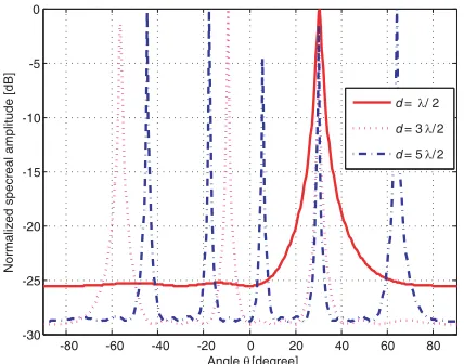
For ULAs, inter-element spacing is fixed as half-wavelength. The purpose is to avoid the problem of phase ambiguity, but at the cost of sacrificing the potential of higher resolution [12]. Let us investigate the influence of different inter-element spacings. Fig. 1 depicts the normalized MUSIC spectrum of ULA for one source with different inter-element spacings, whereM = 4, θ= 30◦, SNR = 0 dB, and the inter-element spacing d is set as λ/2, 3λ/2, and 5λ/2, respectively. As is shown, when d = λ/2, the spectrum has only one but wide peak, i.e., no ambiguity but with low resolution. As dincreases, more sharper peaks can be observed, i.e., estimation resolution is enchanted. However, except for the peak at the true DOA, multiple virtual peaks are also generated, i.e., the problem of phase ambiguity arises. Since sparse array with larger inter-element spacing can provide a higher resolution, we consider to extract the SULAs from the conventional half-wavelength ULA. Let’s uniformly extract

integer operation. The inter-element spacing d = βsλ₂ , and βs(>1) is an integer. According to the

limitation in ULA, (Ms−1)βsλ2 ≤(M−1)λ2 such that the size of the SULA is no bigger than that of

the original ULA. Therefore, the maximum value βs with respect toMs is given by

β_smax= M −1

Ms−1

(8)

where · stands for the round down to the nearest integer operation.

For the SULA, the steering vector for the kth source can be similarly given as

a_s(θk) =

1, e−jβsmaxπsin(θk)_{, . . . , e}−j(Ms−1)βsmaxπsin(θk) _T

(9)

Then the sample estimate of array covariance matrix R_x,s=Ex_s(t)xH_s (t)is given by

R_x,s,e= 1

T T

t=1

x_s(t)xH_s (t) (10)

wherex_s(t) is the received signal and the EVD of R_x,s,e is

R_x,s,e =E_s,s,eΛ_s,s,eEH_s,s,e+E_n,s,eΛ_n,s,eEH_n,s,e (11) whereE_s,s,e andE_n,s,eare the estimated signal- and noise- subspace matrices, respectively.

3.2. Relation Among True and Virtual DOAs

For the Ms-element SULA with d = β

max

s λ

2 , there exist multiple peaks for each source DOA in the

MUSIC spectrum, as shown in Fig. 1. Assume θv,k denotes one of the virtual DOAs with respect to

the true DOA θk. Since both θk and θv,k generate the same peaks in the MUSIC spectrum, they must

satisfy that 2_λπdsinθk−2_λπdsinθv,k= 2nπ, i.e.,

sinθk−sinθv,k=

2n βmax

s

(12)

where n is an integer [12, 14]. When d ≤ λ₂, there is no virtual DOA that satisfies Equation (12). Therefore, there exists only one peak for each DOA. However, when d > λ₂, multiple peaks will be generated, among which only one is the estimation of true DOA. In the sine domain, the true value

-80 -60 -40 -20 0 20 40 60 80

-30 -25 -20 -15 -10 -5 0

Angle θ [degree]

Normalized specreal amplitude [dB]

d=λ/ 2

d= 3 λ/ 2

d= 5 λ/ 2

Figure 1. Normalized MUSIC spectrum in angle domain with d = λ/2, 3λ/2, and 5λ/2, respectively.

-1 -0.8 -0.6 -0.4 -0.2 0 0.2 0.4 0.6 0.8 1 -30

-25 -20 -15 -10 -5 0

sin(θ)

Normalized specreal amplitude [dB]

d= λ/ 2

d= 3 λ/ 2

d= 5 λ/ 2

sinθkand virtual value sinθv,khave the difference ofn×_βsmax2 . According to−1≤sinθ≤1, there exists

at mostβ_smax virtual peaks.

In the sine domain, all the peaks for each DOA are uniformly distributed, which is illustrated in Fig. 2. According to the linear relation, we can recover all the peaks if an arbitrary one is acquired. Based on the property, we study the DOA estimation by utilizing the sparse structure and the linear relation among true DOA and virtual DOAs.

3.3. The Proposed Estimation Method

According to the relation in Equation (12), we equally divide the total field-of-view in sine domain into

β_smax small sectors φn, n= 1,2, . . . , β_smax, i.e.,

φn=

−1+2 (n−1)

βmax s

,−1+ 2n

βmax s

(13)

The length of each sector is _βsmax2 . It can be seen clearly from Equation (12) that for each true DOAθk,

there exists one spectral peak in each sector simultaneously, i.e., one true DOA and β_smax−1 virtual DOAs. The virtual DOAs together with the true DOA are uniformly distributed in the sine domain.

Therefore, we can search over an arbitrary sector φn, n = 1,2, . . . , βmax_s to find the K (true or virtual) peaks for all the sources in the sine domain, denoted as

Pest_s,n=sinθest1,n,sinθest2,n, . . . ,sinθK,nest

(14)

According to Equation (12), the peaks in other sectors can be recovered without spectral search. Specially, the peaks inφm, m= 1,2, . . . , β_smax can be recovered as

Pest_s,m=Pest_s,n+ (m−n) 2

βmax s

(15)

Then we have all the virtual (and true) peaks, which is denoted asPest_s = [Pest_s,1,Pest_s,2, . . . ,Pest_s,βsmax].

Since the phase ambiguity problem is caused by the large inter-element spacing, it cannot be eliminated by the SULA itself. Note that the steering vector a(θ) of the original ULA is orthogonal to the original noise-subspace E_n,e only at true DOAs and non-orthogonal at the virtual DOAs. Therefore, we can select the K true DOAs among Kβ_smax virtual values vector Pest_s by finding the maximum peaks of 1/EH_n,ea(θ)2. The positions of the selected peaks in sine domain is denoted as Pest_s,sel= [pest1 , pest2 , . . . , pestK ], wherepesti ∈Pests , i= 1,2, . . . , K.

Finally, the true DOAs can be estimated by

θ_iest= arcsinpest_i , i= 1,2, . . . , K (16) Instead of searching over the total angular field-of-view, the proposed method involves a limited spectral search over a small sector. Then the other virtual (or true) DOAs can be computed immediately without spectral search. Therefore, the proposed method is quite computationally efficient.

Remark 1: In the considered sparse model, to apply the MUSIC algorithm inMs-element SULA, at

least one eigenvector from the EVD of the covariance matrix is left to span the related noise subspace, thus the number of sources can be detectable is Ms−1, while the M-element ULA can detect up to M −1 sources. Therefore the maximum number of detectable sources is reduced; however, it is to be shown that this reduction can lead to a much lower computation complexity and a better estimation accuracy and complexity tradeoff as compared to the standard MUSIC.

4. COMPLEXITY ANALYSIS

In this section, we analyze the computational complexity of the proposed method and compare it with that of the standard MUSIC as well as the compressed MUSIC (C-MUSIC) in [10].

For the proposed method, it has to compute EH_n,s,ea_s(θ)2 for each spectral point. Note that the dimension ofE_n,s,eisMs×(Ms−K) and the proposed method involves a limited search over only one

small sector with J/βmax

flops. The EVD step of R_x,s,e needs M_s2(K+ 2) flops [7]. Moreover, the proposed method requires an additional check step for K ×β_smax virtual DOAs and it has to compute EH_n,ea(θ)2 for each virtual DOA. The check step requiresKβ_smaxM(M−K) flops. Therefore, the total computational complexity of the proposed method is given by

Cproposed=JMs(Ms−K)/βsmax+Ms2(K+ 2) +KβsmaxM(M−K) (17)

For the standard MUSIC, it has to computeEH

n,ea(θ)2for each spectral point. Hence, the spectral

step needsJM(M−K) flops. The computational complexity is given as

CM U SIC =JM(M−K) +M2(K+ 2) (18)

For C-MUSIC,JM(M −β_smaxK)/β_smaxflops are required by the spectral search step andM_s2(K+2) flops are required for FSD. Additionally, it needs a SVD step for a M ×M matrix, which requires

M2_(βmax

s K+ 2) flops. Therefore, the computational complexity is given by

CC-M U SIC =M2(K+ 2) +M2(βsmaxK+ 2) +JM(M−βmaxs K)/βsmax (19)

For the sake of clarity, the computational complexities of all the above methods are summarized in Table 1. It can be easily seen that the complexity of the proposed method is significantly lower than that of other methods.

Table 1. Comparison of computational complexity.

Proposed Method JMs(Ms−K)/βsmax+Ms2(K+ 2) +KβsmaxM(M −K)

C-MUSIC M2(K+ 2) +M2(β_smaxK+ 2) +JM(M−β_smaxK)/β_smax

MUSIC JM(M −K) +M2(K+ 2)

For spectral search step 0.01◦, the number of search points is J = 180◦/0.01◦ = 1.8×104. When

M = 13,Ms= 7,βsmax= MsM−−11= 2, and the inter-element spacingd= βmaxs λ

2 =λ, the complexities of

the standard MUSIC and C-MUSIC are computed as 2.57×106 _{and 1.05×10}6 _{flops, respectively. The}

complexity of the proposed method is 3.16×105 flops. Hence, the complexity of the proposed method is about 12.3% of that of the standard MUSIC and is about 29.9% of that of the C-MUSIC method. Obviously, regarding the implementation, our proposed method is significantly of lower complexity than other methods. Fig. 3 shows the computational complexity versus for the three methods. We can see that the complexity of the proposed method is much lower than that of other methods.

5. SIMULATION RESULTS

In this section, we compare the performance of the proposed method via simulations with that of other methods, including MUSIC, C-MUSIC, and Minimum Norm (MN) [23]. We consider a ULA with

M = 13 sensors and K = 2 independent narrowband sources. The compression times for C-MUSIC is

β=2. The searching step is set as 0.01◦. The root mean square error (RMSE), expressed as

RM SE =

1

QK Q

q=1 K

k=1

(ˆθk(q)−θk)2

is used as the performance metric, where ˆθk(q) is the estimate of θk for theqth trial, q = 1,2, . . . , Q.

3 4 5 6 7 100

102 104 106 108

M_s

Complexity

Proposed C-MUSIC MUSIC

Figure 3. The complexities of different methods versusMs, whereM = 13.

-10 -8 -6 -4 -2 0 2 4 6 8 10

10-3 10-2

SNR [dB]

RMSE [rad]

Proposed,M_s=4

Proposed,M_s=5

Proposed,M s=7 MUSIC,M =13 C-MUSIC Minimum Norm

Figure 4. RMSEs versus the SNR with two sources, where the snapshot number T = 200.

0 100 200 300 400 500 600 700 800 900 1000 10-3

10-2

Snapshot Number

RMSE [rad]

Proposed,M_s=4

Proposed,M_s=5

Proposed,M s=7 MUSIC,M =13 C-MUSIC Minimum Norm

Figure 5. RMSEs versus the Snapshot Number with two sources, where SNR = 0 dB.

5.1. Comparison of RMSEs

In this simulation, we firstly considerK= 2 sources with their DOAs randomly generated in the range of [10◦,11◦] and [40◦,41◦], respectively.

We compare the RMSEs for DOA estimation by the proposed method with those by other methods in Fig. 4, where the SNR varies from−10 dB to 10 dB. The parameterMs is selected approximately for

the performance comparison. It is observed that both MUSIC and C-MUSIC provide very close RMSE performance, while the performance of the proposed method is slightly worse. However, as compared to MN, the proposed method can improve the performance obviously. With the increase of Ms, the

differences of RMSEs among the proposed method, MUSIC, and C-MUSIC decrease dramatically. Note that when Ms=7, the complexity of the proposed method is only about 12.3% of that of MUSIC and

about 29.9% of that of C-MUSIC. Therefore, the proposed method shows a better estimation accuracy and complexity tradeoff as compared to other methods.

-10 -8 -6 -4 -2 0 2 4 6 8 10 10-3

10-2

SNR [dB]

RMSE [rad]

Proposed,M_s=4

Proposed,M_s=5

Proposed,M_s=7

MUSIC,M =13 C-MUSIC Minimum Norm

Figure 6. RMSEs versus the SNR with three sources, where the snapshot number T = 200.

0 100 200 300 400 500 600 700 800 900 1000 10-3

10 -2

Snapshot Number

RMSE [rad]

Proposed,M_s=4

Proposed,M_s=5

Proposed,M_s=7

MUSIC,M =13 C-MUSIC Minimum Norm

Figure 7. RMSEs versus the Snapshot Number with three sources, where SNR = 0 dB.

-10 -5 0 5 10 15 20 25 30

0 0.2 0.4 0.6 0.8 1 SNR [dB] Resolution Probability

Proposed,M_s=4

Proposed,M_s=5

Proposed,M s=7 MUSIC,M =13 C-MUSIC Minimum Norm

Figure 8. Resolution probabilities versus the SNR, where the snapshot numberT = 200.

0 50 100 150 200 250 300 350 400

0 0.2 0.4 0.6 0.8 1 Snapshot Number Resolution Probability

Proposed,M_s=4

Proposed,M s=5 Proposed,M_s=7

MUSIC,M =13 C-MUSIC Minimum Norm

Figure 9. Resolution probabilities versus the snapshot number, where SNR = 15 dB.

5.2. Comparison of Resolution Probability

In this simulation, we compare the resolution probabilities of different methods in Figs. 8 and 9, where two closely spaced sources are at the DOAs θ1 = 20◦ and θ2 = 22◦, respectively. The two sources are

said to be successfully resolved if and only if [24]

f(θ1) +f(θ2)

2 > f

θ1+θ2

2

(20)

wheref denotes the spectral value.

Figure 9 plots the resolution probability versus the snapshot number with SNR = 15 dB. As is shown, with the increase of T, the resolution performance of the proposed method is improved. The resolution performance is also improved with the decrease of Ms. The resolution probability is slightly

worse than that of both MUSIC and C-MUSIC, especially when the inter-element spacing is large. To see more clearly, we plot the resolution performance against the interval Δθ of the two sources in Fig. 10. We set θ1 = 20◦ and θ2 = θ1 + Δθ, where Δθ varies from 0.2◦ to 3◦. The SNR is set as

15 dB andT = 200. As is shown, MN exhibits the best ability all the methods, especially when the two sources are very close, which is at the cost of higher MSE. As compared to MUSIC and C-MUSIC, the proposed method shows better performance when Δθ is small and worse when Δθ is large. Regarding the complexity, the proposed method makes an efficient trade-off between complexity and resolution.

0 0.5 1 1.5 2 2.5 3

0 0.2 0.4 0.6 0.8 1

Δθ [degree]

Resolution Probability

Proposed,M_s=4

Proposed,M_s=5

Proposed,M_s=7

MUSIC,M =13 C-MUSIC Minimum Norm

Figure 10. Resolution probabilities versus Δθ, whereθ1 = 20◦, θ2=θ1+ Δθ.

-80 -60 -40 -20 0 20 40 60 80

10-3 10-2 10-1 100

Normalized specreal amplitude [dB]

Proposed MUSIC

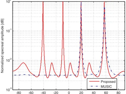
Figure 11. Spectrum of the proposed method and the MUSIC method, where θ1 = 20◦, θ2 =

57.35◦. The two sources generate overlapped spatial spectrum for the SULA.

5.3. Comparison of Spatial Spectrum with Overlapped Virtual DOAs

Since multiple virtual DOAs can be generated for each true DOA, it is possible that two well-separated sources generate the overlapped spatial spectrum for SULA. In this simulation, we fix Ms = 4 and

β_smax = 4. We consider K = 2 sources, whose DOAs are set as θ1 = 20◦ and θ2 = 57.35◦. Since

sinθ2−sinθ1 ≈0.5 =_βmax_s2 , the two sources generate the overlapped spatial spectrum in SULA.

Figure 11 depicts the spatial spectrum for the two sources. As is shown, there are only β_smax= 4 virtual DOAs in such scenario, i.e., one of the virtual sources ofθ1 overlaps the true source θ2, and vice

versa. However, according to the fact that only the steering vectors associated with the true DOAs are orthogonal to the noise subspace of the original ULA, the true DOAs can be uniquely estimated by maximizing 1/EH_n,ea(θ)2. The performing results of orthogonality check is shown in Table 2. We can see that the overlapped DOAs can be estimated successfully by the orthogonality check.

Table 2. Orthogonality check.

angle θˆ1 θˆ2 θˆ3 θˆ4

Candidate DOAs −41.15◦ −9.09◦ 20.0◦ 57.35◦

1EH_n,ea(θ)2 0.0777 0.0774 24.2703 17.2445

6. CONCLUSIONS

In this paper, a computationally efficient DOA estimation method is proposed for uniform linear arrays (ULAs), which exploits the advantage of the sparse structure. For the sparse uniform linear array extracted from the ULA, the MUSIC spectrum can generate multiple peaks at the true DOAs and several virtual DOAs, the steering vectors of which are simultaneously orthogonal to the noise subspace of the sparse array. Based on the relationship among true and virtual DOAs, the proposed method involves a limited spectral search and others can be recovered without spectral search, hence it is computationally efficient. The true DOAs can be distinguished by the original noise subspace of the ULA. It is shown by simulation results that the proposed method has a much lower complexity at the cost of reducing the estimation accuracy slightly. Hence the proposed method achieves a better accuracy and complexity trade-off as compared to other existing estimation methods.

ACKNOWLEDGMENT

This work was supported in part by Shandong Province High School Science & Technology Fund Planning Project (J12LN02), Research Fund for the Doctoral Program of Higher Education of China (20123702120016), and Key Projects in the National Science & Technology Pillar Program during the Twelfth Five-year Plan Period (2011BAD32B02).

REFERENCES

1. Krim, H. and M. Viberg, “Two decades of array signal processing research: The parametric approach,”IEEE Signal Processing Magazine, Vol. 13, No. 4, 67–94, 1996.

2. Jiang, J., F. Duan, J. Chen, Y. Li, and X. Hua, “Mixed near-field and far-field sources localization using the uniform linear sensor array,”IEEE Sensors Journal, Vol. 13, No. 8, 3136–3143, 2013. 3. Capon, J., “High-resolution frequency wavenumber spectrum analysis,” Proceedings of the IEEE,

Vol. 57, No. 8, 1408–1418, 1969.

4. Schmidt, R. O., “Multiple emitter location and signal parameter estimation,” IEEE Transactions

on Antennas and Propagation, Vol. 34, No. 3, 276–280, 1986.

5. Rao, B. D. and K. V. S Hari, “Performance analysis of root-MUSIC,” IEEE Transactions on

Acoustics, Speech and Signal Processing, Vol. 37, No. 12, 1939–1949, 1989.

6. Roy, R. and T. Kailath, “ESPRIT — Estimation of signal parameters via rotational invariance techniques,” IEEE Transactions on Acoustics, Speech and Signal Processing, Vol. 37, No. 7, 984– 995, 1989.

7. Xu, G. and T. Kailath, “Fast subspace decomposition,” IEEE Transactions on Signal Processing, Vol. 42, No. 3, 539–551, 1994.

8. Yan, F., M. Jin, S. Liu, and X. Qiao, “Real-valued MUSIC for efficient direction estimation with arbitrary array geometries,” IEEE Transactions on Signal Processing, Vol. 62, No. 6, 1548–1560, 2014.

9. Barabell, A., “Improving the resolution performance of eigenstructure-based direction-finding algorithms,” Proc. ICASSP’83, Vol. 8, 336–339, 1983.

10. Yan, F., M. Jin, and X. Qiao, “Low-complexity DOA estimation based on compressed MUSIC and its performance analysis,”IEEE Transactions on Signal Processing, Vol. 61, No. 8, 1915–1930, 2013.

11. Morabito, A. F., T. Isernia, and L. Di Donato, “Optimal synthesis of phase-only reconfigurable linear sparse arrays having uniform-amplitude excitations,”Progress In Electromagnetics Research, Vol. 124, 405–423, 2012.

12. Wang, J., D. Vasisht, and D. Katabi, “RF-IDraw: Virtual touch screen in the air using RF signals,”

ACM SIGCOMM14, 235–246, 2014.

13. Vaidyanathan, P. and P. Pal, “Sparse sensing with co-prime samplers and arrays,” IEEE

14. Zhou, C., Z. Shi, Y. Gu, and X. Shen, “DECOM: DOA estimation with combined MUSIC for coprime array,” Proc. WCSP 2013, 1–5, 2013.

15. Weng, Z. and P. Djuric, “A search-free DOA estimation algorithm for coprime arrays,” Digital

Signal Processing, Vol. 24, 27–33, 2014.

16. Shen, Q., Y. Zhang, and M. G. Amin, “Generalized coprime array configurations for direction-of-arrival estimation,”IEEE Transactions on Signal Processing, Vol. 63, No. 6, 1377–1390, 2015. 17. Tan, Z., Y. C. Eldar, and A. Nehorai, “Direction of arrival estimation using co-prime arrays: A

super resolution viewpoint,”IEEE Transactions on Signal Processing, Vol. 62, No. 21, 5565–5576, 2014.

18. Shen, Q., W. Liu, W. Cui, S. Wu, Y. Zhang, and M. G. Amin, “Low-complexity direction-of-arrival estimation based on wideband co-prime arrays,” IEEE/ACM Transactions on Audio, Speech and

Language Processing (TASLP), Vol. 23, No. 9, 1445–1453, 2015.

19. Yin, J. and T. Chen, “Direction-of-arrival estimation using a sparse representation of array covariance vectors,”IEEE Transactions on Signal Processing, Vol. 59, No. 9, 4489–4493, 2011. 20. He, Z., Z. Zhao, Z. Nie, P. Tang, J. Wang, and Q. Liu, “Method of solving ambiguity for sparse

array via power estimation based on MUSIC algorithm,”Signal Processing, Vol. 92, 542–546, 2012. 21. He, J. and Z. Liu, “Extended aperture 2-D direction finding with a two-parallel-shape-array using propagator method,” IEEE Antennas and Wireless Propagation Letters, Vol. 8, No. 4, 323–327, 2009.

22. Stoica, P. and A. Nehorai, “MUSIC, maximum likelihood, and Cramer-Rao bound,” IEEE

Transactions on Acoustics, Speech and Signal Processing, Vol. 37, No. 5, 720–741, 1989.

23. Krim, H., P. Forster, and J. G. Proakis, “Operator approach to performance analysis of root-MUSIC and root min-norm,”IEEE Transactions on Signal Processing, Vol. 40, No. 7, 1687–1696, 1992.

24. Zhang, Q. T., “Probability of resolution of the MUSIC algorithm,” IEEE Transactions on Signal