Numerical Simulation of Three-Phase Flows in the Inverse Fluidized bed

(1)

Scholarship@Western

Electronic Thesis and Dissertation Repository

9-12-2018 3:00 PM

Numerical Simulation of Three-Phase Flows in the Inverse

Fluidized bed

Yunfeng Liu

The University of Western Ontario

Supervisor Zhang, Chao

The University of Western Ontario Co-Supervisor Zhu, JingXu

The University of Western Ontario

Graduate Program in Mechanical and Materials Engineering

A thesis submitted in partial fulfillment of the requirements for the degree in Master of Engineering Science

Follow this and additional works at: https://ir.lib.uwo.ca/etd

Part of the Mechanical Engineering Commons

Recommended Citation Recommended Citation

Liu, Yunfeng, "Numerical Simulation of Three-Phase Flows in the Inverse Fluidized bed" (2018). Electronic Thesis and Dissertation Repository. 5730.

https://ir.lib.uwo.ca/etd/5730

This Dissertation/Thesis is brought to you for free and open access by Scholarship@Western. It has been accepted for inclusion in Electronic Thesis and Dissertation Repository by an authorized administrator of

(2)

i

The inverse three-phase fluidized bed has excellent potentials to be used in chemical,

biochemical, petrochemical and food industries because of its high contact efficiency

among each phase which leads to a good mass and heat transfer. The understanding of the

hydrodynamics and flow structures in inverse three-phase fluidized beds is important for

the design and scale up purposes.

A CFD model based on the Eulerian-Eulerian (E-E) approach coupled with the kinetic

theory of the granular flow is successfully developed to simulate an inverse three-phase

fluidization system. The proposed CFD model for the inverse three-phase fluidization

system is validated by comparing the numerical results with the experimental data.

Investigations on the hydrodynamics and flow structures in the inverse three-phase

fluidized bed under a batch liquid mode are conducted by numerical studies. The

development of the fluidization processes and the general gas-liquid-solids flow structures

under different operating conditions are further studied by the proposed three-phase E-E

CFD model. Parametric studies including different inlet superficial gas velocities, particle

densities, and solids loadings are investigated numerically. The numerical results show a

general non-uniform radial flow structure in the inverse three-phase fluidized bed. It is also

found that the particle distribution profiles in the axial direction relate to the solids loading,

particle density and inlet superficial gas velocity. The existences of the liquid and solids

recirculation inside the inverse three-phase fluidized bed are also noticed under the batch

liquid mode.

Moreover, the proposed CFD model for the inverse three-phase fluidized bed is further

modified by adjusting the bubble size. The modified CFD model takes the bubble size

effects into account and performs better on estimating the average gas holdup. In addition,

a correlation between the bubble size and the superficial gas velocity, gas holdup and

physical properties of the liquid and solid phases is proposed based on the numerical

results. The predicted bubble size and the gas holdup in the inverse three-phase fluidized

beds under a batch mode using the proposed correlation agree well with the experimental

(3)

ii

size adjustment can be used to predict the performance of the inverse three-phase

fluidization system more accurately.

Keywords: computational fluid dynamic (CFD), inverse fluidized bed, three-phase flow,

(4)

iii

Co-Authorship Statement

Chapter 3 and Chapter 4 of this thesis will be submitted for publications.

All papers are drafted by Yunfeng Liu and modified under the supervision of Prof. Chao

Zhang and Prof. Jesse Zhu and in consultation with Miss Zeneng Sun in Prof. Chao Zhang’s

(5)

iv

Acknowledgement

I would like to take this opportunity to express the gratitude and appreciation to those who

have always been helping and supporting me throughout my master’s study.

First, I would like to express my sincerest thank to my Supervisor Prof. Zhu and Prof.

Zhang, for believing my potential, providing me advice, support and encouragement

through my entire research work. I attribute the thesis to their guidance and efforts, which

ensured the work to be successfully completed.

Then I would like to thank all members of our Computational Fluid Dynamics Research

Laboratory, especially Zeneng Sun, Huirui Han, Hao Luo for their help and friendship in

both academic and daily life.

Finally, I would like to thank my parents for their encouragement and support during the

(6)

v

Nomenclature

Notation

𝐶_1𝜀 Turbulence constants, dimensionless

𝐶2𝜀 Turbulence constants, dimensionless

𝐶3𝜀 Turbulence constants, dimensionless

𝐶_𝐷 Drag coefficient, dimensionless

𝑑_𝑝 Mean particles diameter, m

𝑑𝑏 Mean bubble size, m

D Column diameter, m

𝑒 Restitution coefficient for particle-particle collision, dimensionless

ɡ Acceleration due to gravity, m/s2

𝑔0 Radial distribution function, dimensionless

𝐺_𝑏 Generation of turbulence kinetic energy due to buoyancy, m2/s2

𝐺𝑘 Generation of turbulence kinetic energy due to the mean velocity gradients, m2/s2

H Column height from bottom to top, m

𝑘 Turbulent kinetic energy, m2_/s2

𝐾 Interphase momentum exchange coefficient, kg/m3s

𝑝 Pressure, Pa

𝑅𝑒 Reynolds number, dimensionless

(11)

x Ug Superficial gas velocity, m/s

𝑣 Velocity, m/s

x Radial position from left wall to right wall, m

Greek letters

𝛼 Local volume fraction, dimensionless

𝜀 Turbulent energy dissipation rate, m2/s2

𝜀𝑔 Gas holdup, dimensionless

𝛾 Collision dissipation rate of energy, kg/ms3

𝑘Θ𝑠 Granular conductivity, kg/m3s

Θ Granular temperature, m2/s2

𝜆 Bulk viscosity, kg m/s

𝜇 Dynamic viscosity, kg/m-s

𝜌 Density kg/m3

𝜏 Stress sensor, Pa

Subscripts

𝑙 Liquid phase

𝑔 Gas phase

(12)

xi

List of Tables

Table2.1 Operating conditions and physical properties of the liquid, gas and solid phases

... 29

Table 2.2 Parameters of the RNG k-ɛ models ... 35

Table 2.3 Mesh information for the grid independent test... 39

Table 2.4 Average gas holdups for different meshes ... 39

Table 3.1 Operating conditions and physical properties of each phase ... 84

Table 3.2 Parameters of the dispersed RNG k-ɛ models ... 89

Table 3.3 Constitutive equations of the solid phases ... 90

Table 3.4 Mesh information for the grid independent test... 94

Table 3.5 Average gas holdups from different meshes... 94

(13)

xii

List of Figures

Figure 1.1 Schematic diagram of the gas-liquid-solid three-phase fluidization (Muroyama

& Fan, 1985) ... 4

Figure 1.2 Flow regimes in the three-phase inverse fluidized bed. (Fan et al., 1982) ... 6

Figure 1.3 Flow regime map of the three-phase bubble column under the batch mode (Sun,

2017) ... 7

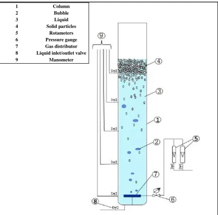
Figure 2.1 Configuration of the experimental setup of the inverse three-phase fluidized bed

(Sun, 2017) ... 28

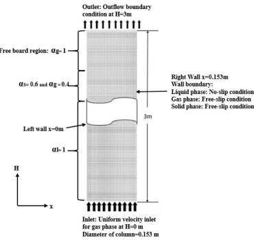
Figure 2.2 Computational domain of the inverse three-phase fluidized bed ... 38

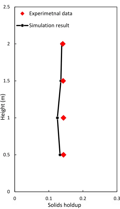
Figure 2.3 Comparison of the axial profiles of the solids volume fraction between the

numerical results and experimental data at Ug=15 mm/s, 15% loading and ρs=930 kg/m3

... 40

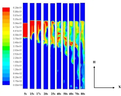
Figure 2.4 Contours of the solids volume fraction at different time of the initial fluidization

stage for Ug=15mm/s, 15% solids loading and ρs= 930 kg/m3 ... 41

Figure 2.5 Axial profiles of the solids volume fraction at different time at the initial

fluidization stage ... 42

Figure 2.6 Radial profiles of the solids volume fraction at different axial locations at the

initial fluidization stage (t=30s). ... 43

Figure 2.7 Radial profiles of the gas volume fraction at different axial locations at the initial

fluidization stage (t=30s) ... 44

Figure 2.8 Radial profiles of the solids axial velocity at different axial locations at the initial

fluidization stage (t=30s) ... 45

(14)

xiii

Figure 2.10 Contours of the solids volume fraction at different time at the developing stage

... 46

Figure 2.11 Axial profiles of the solids volume fraction at different time at the developing

stage (t=150s) ... 47

Figure 2.12 Radial profiles of the gas volume fraction at different axial locations at the

developing stage (t=150s) ... 48

Figure 2.13 Radial profiles of the solids volume fraction at different axial locations at the

developing stage (t=150s) ... 48

Figure 2.14 Radial profiles of the solids axial velocity component at different axial

locations at the developing stage (t=150s) ... 49

Figure 2.15 Contours of the solid phase volume fraction at the fully developed stage with

time ... 50

Figure 2.16 Time-averaged axial profile of the solids volume fraction at the fully developed

stage ... 51

Figure 2.17 Time-averaged axial profile of the gas volume fraction at the fully developed

stage ... 51

Figure 2.18 Time-averaged radial profiles of the solids axial velocity at different axial

locations ... 53

Figure 2.19 Time-averaged radial profiles of the solids volume fraction at different axial

locations ... 53

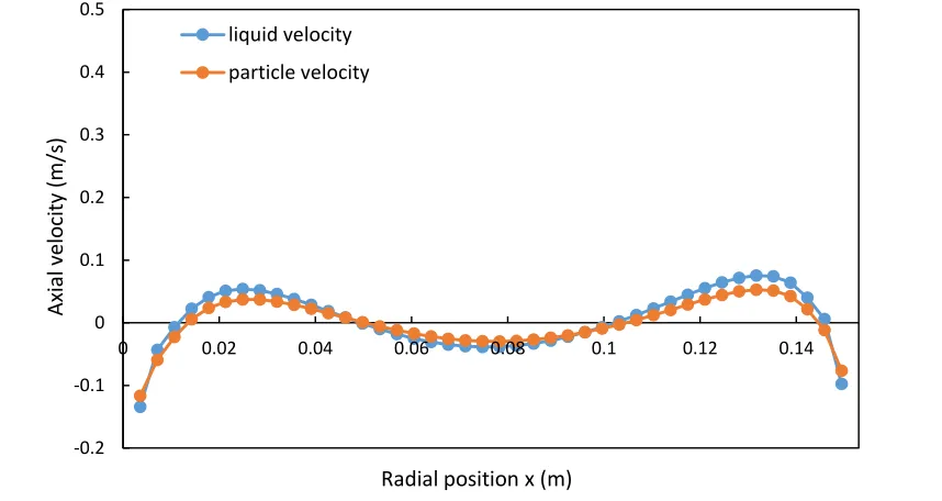
Figure 2.20 Time-averaged radial profiles of the solid and liquid axial velocities at H=1m

... 54

(15)

xiv

Figure 2.22 Axial profiles of the solids volume fraction under different solids loadings at

Ug=15mm/s and ρs=930kg/m3... 56

Figure 2.23 Radial profiles of the solids axial velocity under different solids loadings at

Ug=15mm/s and ρs=930kg/m3... 57

Figure 2.24 Radial profiles of the solids volume fraction under different solids loadings at

Ug=15mm/s and ρs=930kg/m3 ... 58

Figure 2.25 Radial profiles of the gas hold up at Ug=15mm/s and ρs=930kg/m3 ... 59

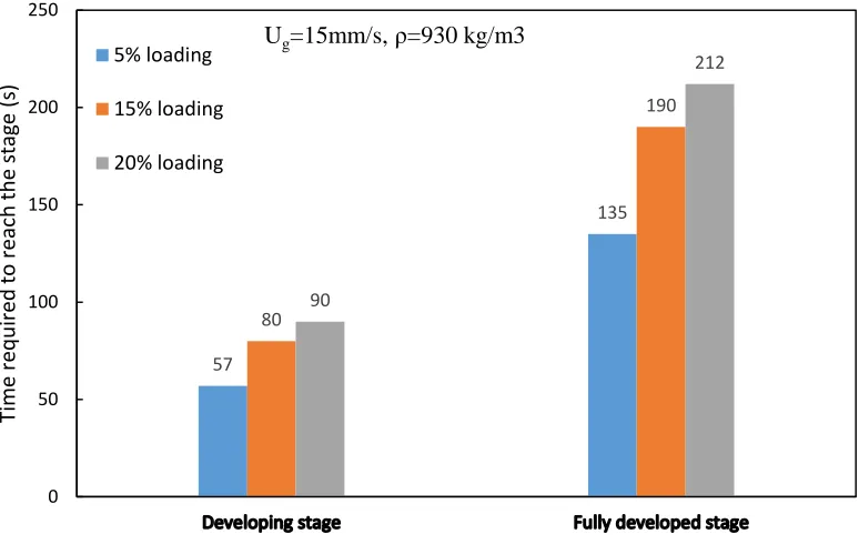
Figure 2.26 Time required to reach to the developing and fully developed stages under

differet inlet superficial gas velocities ... 60

Figure 2.27 Contours of the solids volume fraction under different inlet superficial

velocities at 15% solids loading and ρs=930 kg/m3 ... 63

Figure 2.28 Radial profiles of the solids volume fraction under different inlet superficial

gas velocities ... 64

Figure 2.29 Average gas holdup under different particle densities at Ug=15mm/s, and 15%

solids loading ... 65

Figure 2.30 Contours of the solids volume fraction with different particle densities at 15%

solids loading and Ug=15mm/s ... 66

Figure 2.31 Radial profiles of solids holdup with different particle densities at 15% solids

loading and Ug=15mm/s ... 68

Figure 2.32 Radial profiles of the solids axial velocity under different inlet superficial gas

velocities ... 70

Figure 2.33 Instantaneous volume fraction contour (left) and particle velocity vector

(16)

xv

Figure 3.1 Configuration of the experimental setup of the inverse three-phase fluidized bed

(Sun, 2017) ... 83

Figure 3.2 Computational domain of the inverse three-phase fluidized bed under the batch

liquid mode ... 93

Figure 3.3 Comparison of the average gas holdup between the numerical results and

experimental data under the different inlet superfical gas velocities at 15% solids loading

and ρs=930 kg/m3 ... 96

Figure 3.4 Comparison of the axial gas holdups from the origin CFD model and modified

CFD model with the experiment data at ρs=930 kg/m3 and 15% solids loading ... 98

Figure 3.5 Time-averaged radial gas holdups under different superficial gas velocities from

the modified CFD model ... 99

Figure 3.6 Comparison of the radial profiles of the gas holdup between the origin CFD

(17)

Chapter 1 1 Introduction

1.1 Background

Fluidization is a process that makes the solid particles behave like fluid by introducing

liquid or gas flow. The concept of the fluidized bed was first proposed for the gasification

of coal in the 1920s, and the fluidization was used for fluid catalytic processes (FCC) in

1940s (Werther, Hartge, & Heinrich, 2014). Today, fluidized beds are widely used in

chemical, biochemical, petrochemical and food industries because of the good heat and

mass transfer.

Usually, fluidized beds can be categorized by the fluidizing agent, so that there are

liquid-solid two-phase fluidization, gas-liquid-solid two-phase fluidization and gas-liquid-liquid-solid (GLS)

three-phase fluidization. Gas-solid fluidized beds were the first to be applied in industries,

then the application extended to the liquid-solid and gas-liquid-solid fluidized beds.

With the development of fluidization technology, fluidized beds can also be characterized

by the flow directions after the concept of the inverse fluidized bed was proposed. Fluidized

beds can be further divided into upward fluidized beds and inverse fluidized beds.

For the traditional upward two-phase fluidization process, the liquid or gas is injected into

the reactor from the bottom and flows through the space between particles. Under a low

fluid velocity, the drag force acting on the particles cannot overcome the gravity of particles,

causing them to remain packed. The fluidization begins as the fluid velocity reaches to the

minimum fluidization velocity where the drag force acting on the particles can balance the

gravity of the particles. Minimum fluidization velocity Umf is an important parameter for

designing the fluidized bed (Zhu, Na, & Lu, 2007). By further increasing the fluid velocity,

the drag force acting on particles will increase and particles will entrain out of the fluidized

bed reactor, and the fluidized bed becomes a circulating fluidized bed if the entrained

(18)

For gas-solid upward fluidization, the fluidized bed usually goes through the bubbling

regime, turbulent regime, fast fluidization regime, to the pneumatic transport regime with

the increase in the superficial gas velocity (Grace, 1986). For the gas-liquid-solid

fluidization, the gas phase is usually introduced into the reactor as bubbles. The flow

regime can be divided into dispersed bubble flow, discrete bubble flow, coalesced bubble

flow, slug flow, churn flow, bridging flow and annular flow at different gas and liquid

velocities (Zhang, Grace, Epstein, & Lim, 1997).

As mentioned before, the three-phase GLS fluidized bed has been studied since 1970s with

the development of fluidization technology (Ostergaard, 1971). Due to the close contact

among solid, liquid and gas phases in GLS three-phase fluidized beds (TPFBs), it is used

in chemical and biochemical processing (Muroyama & Fan, 1985). Three-phase

fluidization can be divided into upward flow phase fluidization and inverse

three-phase fluidization depending on the flow direction of the gas and liquid three-phases. The

different modes of three-phase fluidization is shown in Figure 1.1. Modes 1a and 1b are

co-current flows where the air and liquid are injected from the bottom of the reactor and

particles are moving upward. Modes 2a and 2b are countercurrent flows where the gas is

introduced to the reactor from the bottom and the liquid is injected from the top of the

reactor. The density of the particles used for modes 2a and 2b are usually less than the

density of the liquid medium, allowing particles to overcome the buoyancy force and

expand downward during the fluidization process. Besides modes 2a and 2b, the inverse

fluidization can be also operated under the batch liquid mode (Comte, Bastoul, Hebrard,

Roustan, & Lazarova, 1997; Sun, 2017), in which the liquid initially fills the reactor and

the particles are floated at the top surface of the liquid before the operation starts. In the

inverse fluidized bed under the batch mode operating condition, the fluidization state of

the particles can be achieved with the zero liquid velocity when the superficial gas velocity

is high enough resulting in the drag force and gravity acting on particles balanced with the

buoyancy force. Compared to the upward flow phase fluidization, the inverse

three-phase fluidization can reduce energy cost and minimum solids attrition as the solid three-phase

can be fluidized under low liquid and gas velocities, and the particle entrainment problem

can be eliminated without using any external equipment (Ibrahim, Briens, Margaritis, &

(19)

wastewater treatment industries. Compared with the traditional methods of the wastewater

treatment such as activated sludge process which requires longer retention time and large

space, the retention time can be reduced in fluidized bed reactor due to high biomass

concentration, and another problem of excessive growth of biomass on particles can be

fixed by using light particles in inverse fluidized beds as well (Sokół & Korpal, 2006).

Understanding the hydrodynamics of inverse three-phase fluidized beds is important when

designing the reactors for industrial applications. Fan, Muroyama and Chern (1982) first

defined the flow regime for the inverse three-phase fluidized bed, which are the fixed bed

with dispersed bubble regime, bubbling fluidized bed regime, transition regime and

slugging flow regime based on the liquid and gas velocities. Other flow characteristics in

the inverse three-phase fluidized bed including the phase holdup, minimum fluidization

velocity, pressure drop, bubble behavior, bed expansion has been studied by many

researchers (Briens, Ibrahim, Margaritis, & Bergougnou, 1999; Renganathan & Krishnaiah,

2008; Son, Kang, Kim, Kang, & Kim, 2007). However, few researchers have reported the

flow structure in the radial direction of the inverse three-phase fluidized bed.

1a 1b 2a 2b

Continuous phase Diagram of

GLS fluidized

bed

Liquid Gas Liquid Gas

Flow

(20)

Figure 1.1 Schematic diagram of the gas-liquid-solid three-phase fluidization

(Muroyama & Fan, 1985)

Although a few experimental studies on the hydrodynamics in GLS three-phase flows have

been conducted, it is hard to fully understand the underlying phenomena of the GLS

three-phase fluidization due to the complex interactions between each three-phase. There is even less

studies focused on predicting the flow characteristics of the inverse three-phase fluidized

bed due to the restrictions of the experiments. Therefore, with the rapid development of

computer technology, CFD has become a powerful tool to simulate the multiphase flow

and provide more details on the three-phase fluidization process. In addition, CFD is

considered to be more time and economic efficient to simulate complex flows compared

with the experimental method. However, few CFD models has been developed to predict

the hydrodynamics and flow structure in inverse three-phase fluidized beds (TPFBs).

1.2 Literature review

The literature review will focus on two parts, which are the experiment studies on the

hydrodynamics of the GLS three-phase inverse fluidized bed and the CFD simulations of

the GLS three-phase fluidized bed.

1.2.1 Experimental

studies

of

the

hydrodynamic

characteristics of the inverse three-phase fluidized beds

Minimum fluidization velocity is an important parameter to consider when designing an

inverse three-phase fluidized bed. Minimum fluidization velocity is defined as the velocity

when the pressure gradient across the bed is minimum in the inverse three-phase fluidized

bed (Ibrahim et al., 1996). Ibrahim et al.(1996) found that the minimum liquid fluidization

velocity will decrease when increasing the gas velocity. Many researchers also reported the

same trend in which the minimum liquid fluidization velocity decreases with the increase

in gas flowrate (Bandaru, Murthy, & Krishnaiah, 2007; Cho, Park, Kim, Kang, & Kim,

2002; D. H. Lee, Epstein, & Grace, 2000; Renganathan & Krishnaiah, 2008). Renganathan

and Krishnaiah (2008) also found the same results and developed the correlation for the

minimum gas fluidization velocity in inverse three-phase fluidized beds under the batch

(21)

1.2.1.1 Modes of operation and flow regimes

Inverse three-phase fluidized beds can operate under the batch liquid mode or continuous

mode. Under the batch liquid mode, the liquid velocity is zero, and the fluidization state of

particles can be achieved by injecting gas only. The main method to determine the flow

regime for inverse three-phase fluidized beds is by visual observation of the flow

phenomena (particle movement or bubble behavior) in the experiment.

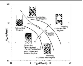
Fan et al. (1982) conducted the first experimental study to investigate the hydrodynamics

in the three-phase inverse fluidized bed. Both the gas and liquid phase can be considered

as the continuous phase in an inverse three-phase fluidized bed. Fan et al. (1982) defined

four flow regimes shown in Figure 1.2 based on the gas and liquid velocities in an inverse

three-phase fluidized bed, which are: (a) the fixed bed with the dispersed bubble regime,

(b) the bubbling fluidized bed regime, (c) the transition regime and (d) the slugging

fluidized bed regime. In the fixed bed with dispersed bubble regime, the gas and liquid

velocities are low, and the drag force and gravity acting on the particle cannot overcome

the buoyancy force. In this regime, the particles remain packed. With the increase in gas

and liquid velocities, the bubbling fluidized bed regime can be reached. The gravity and

drag force exerted on particles can balance the buoyancy force, so, particles start to fluidize

from the bottom of packed bed, ultimately distributing uniformly along the reactor. The

bubble size is uniform within the bubbling fluidized bed regime. At the transition regime,

bubbles starts to coalescence and their sizes will change. At the slugging fluidized bed

regime, particles will move upward with slug bubbles, and then settle down quickly, and

(22)

Figure 1.2 Flow regimes in the three-phase inverse fluidized bed. (Fan et al., 1982)

Only a few researchers studied the batch mode of the inverse three-phase fluidized bed

compared to the continuous mode. Comte et al. (1997) conducted experiments in an inverse

TPFB under the batch mode operating condition. The particles used in the experiment have

a mean density of 934 kg/m3_{, and gas bubbles are introduced into the fluidized bed by using}

a perforate plate and membrane distributor. Three significant transition velocities have

been defined based on different distributions of the solid phase to distinguish the flow

regimes and study the flow behavior: (1) the minimum gas fluidization velocity Ug1 that

can break the fixed bed; (2) velocity Ug2 is the velocity at which some particle can reach

the bottom of the reactor; (3) velocity Ug3, at this velocity, the particle distribution is

uniform along the reactor. It was found that Ug2 and Ug3 will decrease when increasing the

solids loading or particle density. A mathematical model to predict velocity Ug3 was

developed based on the assumption that the particle movement is mainly due to the density

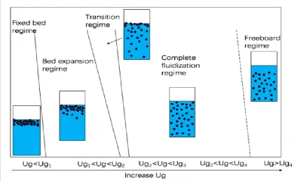
difference between particles and mixture of gas and liquid. Sun (2017) also proposed

similar specific transition velocities, which are the initial fluidization velocity, expansion

(23)

shown in Figure 1.3. In addition, when the superficial gas velocity is above Ug4, a free board

region can be observed. It was also confirmed that Ug1, Ug2 and Ug3 will decrease with the

increase in the particle density. Han et al. (2003) used particles with a density of 934 kg/m3

but the gas distributor used in their experiment is different from the distributor used in the

experimental study by Comte et al. (1997), so a different Ug3 value was derived. Thus, the

gas distributor is one of the factors that can influence the Ug3 (Han et al., 2003). Sun (2017)

further confirmed this fact by using particles with a density of 930 kg/m3_{and the porous}

quartz gas distributor, which can generate small bubbles, obtained the smallest Ug3 value

among the three studies.

Figure 1.3 Flow regime map of the three-phase bubble column under the batch

mode (Sun, 2017)

1.2.1.2 Particle movements

Buffière and Moletta (1999) investigated the influence of the particle size and density on

the flow regimes of the inverse fluidized bed under the batch liquid mode. Two types of

particles are used in the experiment: one has a mean diameter of 4 mm with density of 920

(24)

For larger particles with a constant superficial liquid velocity, particles start to settle down

and accumulate at the bottom of the reactor when the superficial gas velocity increases

which results in a semi-fluidization phenomenon. For smaller particles, it was found that

they will distribute uniformly in the reactor when the gas velocity is above a certain value,

though the particle density is still smaller than the density of the surrounding liquid-gas

mixture. In addition, smaller particles will flow upward with the liquid motion at a high

gas velocity, so there is no semi-fluidization for smaller particles at a high gas velocity. In

that case, two possible particle expansion mechanisms were proposed: (1) the density

difference between particles and liquid-gas mixture and (2) the liquid circulation effect

caused by rising bubbles. Later, Renganathan and Krishnaiah (2008) reported the particle

expansion mechanism as a combination of the density difference effect and liquid

circulation effect. It was indicated that the liquid circulation is not enough to cause the

particle movement if the density difference between particles and the liquid-gas mixture is

very large for large size particles.

1.2.1.3 Phase holdups

Cho et al. (2002) conducted an experiment to find out the average phase holdup of an

inverse TPFB under the continuous operating condition. The results showed the gas and

liquid holdups will increase with an increase in the gas and liquid velocities. Later, Bandaru

et al. (2007) also reported the same trend for the liquid average holdup. Only a few studies

reported the axial distributions of flow parameters for each phase in inverse TPFBs.

Ibrahim et al. (1996) and Bandaru et al. (2007) studied the distribution of the axial volume

fraction of each phase in an inverse TPFB. It was found that the bed remains fixed at a

lower gas and liquid velocity. With the increase in the inlet liquid or gas velocity, the

packed bed starts to fluidize, and the particles begin to move downward. The gas phase

holdup was eventually found to be uniform along the reactor.

Buffière and Moletta (1999) proposed a correlation to predict the liquid holdup and bed

porosity under the batch liquid mode in the inverse TPFB, and it can be used in the

dispersed bubble regime and the transition regime. The gas holdup was found to be

independent of the liquid velocity, and the gas holdup for large particles is higher than that

(25)

not be able to break up the bubble. Sun (2017) reported that the gas holdup increases, and

the liquid holdup decreases with a constant solids loading when increasing the superficial

gas velocity. In addition, it was also reported that the local solids volume fraction in the

axial direction decreases at the top and increases at the bottom of the column gradually

with an increase in the superficial gas velocity.

1.2.1.4 Remarks

Only a few researchers studied the fluidization process in inverse TPFBs. Most particles

remain packed at the minimum fluidization velocity, and the hysteresis effect between the

fluidization and defluidization was also found in inverse TPFBs (D. H. Lee et al., 2000).

Renganathan and Krishnaiah (2008) observed that particles expanded layer by layer from

the bottom of the packed bed instead of expanding suddenly at the minimum fluidization

velocity under the batch liquid operating condition. The bed expansion was found to be

heterogeneous first before reaching to the homogeneous expansion state (K. Il Lee et al.,

2007). It was also found that the bed expands faster when using heavier particles or

increasing gas and liquid velocities in inverse TPFBs.

In an inverse TPFB, the gas is always introduced to the reactor as bubbles, which it is one

of the key factors that can influence the heat and mass transfer. Therefore, it is important

to study the bubble behavior and properties in order to better understand the flow

characteristics of inverse TPFBs. Son et al. (2007) studied bubble properties in an inverse

TPFB, and the results showed that the bubble size increases with an increase in the liquid

or gas velocity. It was also found that the bubble size and the bubble rising velocity is

higher when using the particles with smaller density. The correlation of bubble size, bubble

rising velocity, and frequency was proposed based on the gas drift flux. Cho et al. (2002)

also reported that the bubble size increases with an increase in the gas velocity.

1.2.2 CFD modelling of multiphase flows in fluidized beds

In past decades, with the rapid development of the computer technology, computational

fluid dynamics (CFD) has becomes a powerful tool to simulate multiphase flows as it is

(26)

to simulate multiphase flows: (1) Eulerian-Eulerian approach and (2) Eulerian-Lagrangian

approach.

The Eulerian-Lagrangian approach treats the liquid and gas as a continuous phase by

solving the Navier-Stokes equations, and the solid phase is treated as a discrete phase which

can be solved by tracking the trajectories of each particle based on the Lagrangian force

balance equation (ANSYS, 2014). Compared to the Eulerian-Eulerian approach, the

advantages of the Eulerian-Lagrangian approach are that fewer empirical constitutive

relations need to be used and the detailed information of the discrete phase can be obtained.

Therefore, many researchers used the Eulerian-Lagrangian approach to investigate the flow

characteristics of the discrete phase in micro-scales. Li, Zhang and Fan (1999) studied the

single bubble wake behavior and particle entrainment phenomena in a GLS three-phase

bubble column by using the VOF-DPM (volume of fluid-discrete phase model) which

described the flows of gas bubbles and solid particles in the Lagrangian coordinates and

the liquid phase in the Eulerian coordinates. Later, Zhang and Ahmadi (2005) developed a

CFD model for the GLS slurry fluidized bed based on the Eulerian-Lagrangian method,

and the effect of the bubble size on the flow structure and transient characteristics of the

three-phase flows was studied. Wen, Lei and Huang (2005) treated the liquid and gas

phases as continuous, and solid phase as the discrete phase to study the hydrodynamics in

a TPFB and got a good agreement between the numerical results and experiment data.

Since the Eulerian-Lagrangian approach tracks the trajectory of each individual particle,

one of the fundamental assumptions made for the Eulerian-Lagrangian model is that the

volume fraction of the discrete phase is low (ANSYS, 2014). The computational resource

needed for simulating multiphase flows will be high if the discrete phase volume fraction

is high (Pan, Chen, Liang, Zhu, & Luo, 2016). Although the Eulerian-Lagrangian method

can predict the hydrodynamics of TPFBs accurately and provide more micro-scale

information on the discrete phase, the Eulerian-Eulerian method will be used in the present

work because the solids volume fraction in an inverse TPFB is high.

The Eulerian-Eulerian approach treats all phases as the interpenetrating continuum, and all

phases are solved using governing equations which are closed by additional closure laws

(27)

governing equations for both the gas and liquid phases. Turbulence models used to close

the Reynold-averaged Naiver Stokes can be divided into four categories: (1) zero-equation

turbulence model; (2) one-equation turbulence model; (2) two-equation turbulence model

and (4) RSM (Reynold Stress) turbulence model.

The zero-equation turbulence model is the simplest eddy viscosity model that uses only

one algebraic equation to calculate the turbulence viscosity. So, there are no other partial

differential equations needed to calculate the turbulent stress. The Prandtl’s mixing length

theory was the first zero-equation turbulence model developed in 1920s (Prandtl, 1925)

based on the Bounsinesq hypothesis (Boussinesq, 1877). But it only considered the mean

velocity in a single direction. Later, Cebeci and Smith (1974) and Baldwin and Lomax

(1978) extended the model to describe multi-dimensional turbulent flows. The drawbacks

of the zero-equation turbulence model are the underestimation of the transport effects, and

having difficulties in deriving the turbulence length scale for different types of flows from

the empirical data.

The one-equation turbulence model calculates the turbulent eddy viscosity by solving one

more transport equation for the turbulent kinetic energy. Spallart and Allmaras (1992)

developed a one-equation model, which can predict the free shear and boundary layer flows

correctly. The advantage of the one-equation turbulence model is that less computation

time is required. However, it also has the same drawback as the zero equation turbulence

model in which the accuracy strongly depends on the specified turbulent length scale and

time scale of the flow.

Two-equation turbulence models such as the k model turbulence models are more

popular than the zero and one-equation turbulence models because they overcome the

drawbacks of the zero and one-equation models. The turbulent viscosity can be calculated

by solving two additional transport equations for the turbulence kinetic energy and

turbulence dissipation rate. Launder, Reece, and Rodi (1975) first developed the standard

k turbulence model but it is only valid for high Reynolds number turbulent flows. To be

(28)

and Orszag (1986) developed the RNG k model by adding addition terms and functions

in the transport equation based on the renormalization group theory. Shih et al. (1995)

developed the Realizable k model in order to improve the performance of the standard k  model on predicting flows with a high shear rate and massive separation. The model has

a new transport equation of dissipation rate related to the vorticity fluctuation at a high

Reynolds number and a new formation for the turbulence viscosity based on realizability

constraints. Laborde-Boutet et al. (2009) compared the performance of each turbulence

models by predicting the turbulent flow characteristics in bubble columns. The results

showed that the RNG k has a better performance than the standard and realizable k

models. The study also investigated the influence of using different turbulence models, the dispersed k model, dispersed k  model with bubble induce effect and per phase k 

model to account for the effect of the gas phase turbulence on the liquid phase turbulence.

The results showed there is no influence on the predicted velocity filed, but the turbulent

quantities are higher when accounting for the bubble induced turbulence. Masood and Delgado (2014) reported that both the dispersed RNG k  model and dispersed RNG k 

model with bubble induced turbulence can predict the average velocity and turbulent

accurately in a 3D square bubble column. Hamidipour, Chen, and Larachi (2012) extended

the study to a three-phase bubble column and found the dispersed RNG k  has a better performance on predicting the flow field in TPFBs bed than the per-phase RNG k  model, realizable standard k  model and standard k  model.

The RSM model is a second closure model, which closes governing equations by solving

the transport equation of Reynold stresses instead of calculating the eddy viscosity. The

RSM model has better performance on predicting the anisotropic flows than all other

turbulence models mentioned above. The drawback of the RSM is the computation expense

is high. Therefore, two equation turbulence models are used in the simulation of the

multiphase fluidization in present work.

For the solid phase, the kinetic theory of granular flow (KTGP) proposed by Chapman and

Cowling (1970) is used to model the solid phase pressure, viscosity and stress in order to

(29)

particle-particle collision can be analogous to the random motion of gas molecules in a

thermodynamic system. The granular temperature is defined analogous to the temperature

in a thermodynamic system, which is related the particle velocity fluctuation. The solids

phase viscosity and stress are the functions of the granular temperature. Ding and

Gidaspow (1990) modelled the gas-solid fluidization by using the KTGP. Later, some

researchers also used the KTGP for the solid phase when modeling three-phase fluidization

(Hamidipour et al., 2012; W. Li & Zhong, 2015; Wu & Gidaspow, 2000). Johnson and

Jackson boundary condition (Johnson & Jackson, 1987) was often used for the solid phase

to account for the collisions between the wall and particle, and the specularity coefficient

is an empirical parameter to define the wall condition. The specularity coefficient can vary

from zero to one where one represents the no-slip wall condition which means significant

amount of lateral momentum transfer existed at wall, and zero represents the free-slip wall

condition which means there is no shear at the wall.

For the three-phase fluidization modelling, the Eulerian-Eulerian approach can be

categorized into two types which are the pseudo two-fluid model and three-fluid

Eulerian-Eulerian approach. The pseudo two-fluid model can be used for modeling the three-phase

fluidization only when the gas bubble is smaller than the particle size and uniformly

distributed along the column because the gas phase and fluid phase can be considered as a

single mixed fluid phase (Felice, 2000). In addition, the two-fluid model is also applied to

the three-phase fluidization when the particle size is small enough, the loading is low and

the slip velocity between the solid and liquid phases is small. In that case, the liquid and

solid suspension can be simplified to one-phase, and it is often used in the three-phase

slurry bubble column simulation (Grevskott, Sannaes, Dudukovic, Hjarbo, & Svendsen,

1996; Hillmer & Weismantel, 1994; Wen & Xu, 1998). In addition, Feng et al. (2005)

employed a pseudo two fluid model to the gas–liquid-nanoparticles three-phase

fluidization process, and the results was validated with the experimental data and the

agreement was strong. By applying the pseudo two-fluid model for the three-phase

simulation, the complicated three-phase flows can be simplified to a two-phase flow, which

reduces the computation expanse as well. However, the drawback of the pseudo two-fluid

model is that the application is limited by the particle size and particle loading, and it also

(30)

Eulerian-Eulerian approach will be used because of the large particle size used in the present study.

Only a few literatures presented the CFD modelling based on the three-fluid

Eulerian-Eulerian model as the interactions among each phase is complicated in TPFBs.

Panneerselvam, Savithri, and Surender (2009) developed a CFD model for TPFBs based

on the three-fluid Eulerian approach. Two different reactors were used to validate the

model, and the particle densities are 2475 kg/m3 and 2500 kg/m3. The dispersed standard

k  turbulence model combined with the bubble and gas induced turbulence model on

liquid was applied to the liquid phase. The constant viscosity model (Gidaspow, 1994)

instead of the KTGP was used to describe the solid pressure and stress. Only the drag force

was considered as the interaction force among each phase to calculate the momentum

exchange coefficient. The drag model used between the liquid and solid phases is the

Gidaspow drag model (Gidaspow, 1994). For the liquid and gas phases, the Tomiyama

drag model (Tomiyama, 1998) and Grace drag models (Grace, 1973) were used, and the

Tomiyama drag model gives a better performance by comparing the experimental results.

The drag model used for the gas and particle phases in this study was the Schiller-Naumann

drag model (Schiller & Naumann, 1935). The no-slip wall boundary condition for the liquid

phase and free slip condition for the gas and solid phases were selected. The velocity inlet

and pressure outlet were selected as boundary conditions. The mean bubble size is used

without considering the bubble size distribution in their study (Panneerselvam et al., 2009),

and it was determined by comparing the gas holdup derived from the CFD results using

different bubble sizes with the average gas holdup from the experiment data. The

simulation results showed a good agreement on the axial gas hold, axial solids velocity,

and turbulence quantities such as turbulent velocity and shear stress with the experimental

data. However, the model cannot predict the near wall region correctly.

Hamidipour et al. (2012) presented a CFD model based on a three-fluid model combined

with the KTGP in the same TPFBs as Panneerselvam et al. (2009) to investigate the

performance of different turbulence models and solid wall conditions. A single bubble size distribution assumption was made in this study. The results showed the dispersed RNG k

(31)

three-dimension and two-three-dimensional models are capable of predicting the flow field, but the

three-dimensional model is slightly accurate than the two-dimensional model. However,

the computational cost of the three- dimensional simulation is also high. The no-slip wall

condition for the liquid phase, free-slip for the gas and solids phases were recommended.

The bubble size input for the second phase was found to have an influence on the gas

holdup, and the smaller bubble size resulted in a higher gas holdup. Also, the interphase

force between the continuous and dispersed phases has been studied widely in literatures,

but the interaction between two dispersed phases has not been well understand and modeled.

Hamidipour et al. (2012) used the same method to model the drag force between the two

dispersed phases to model the drag force between the continuous and dispersed phases

because two dispersed phases were also treated as continuums in the Eulerian-Eulerian

approach. The drag model used between the gas and solid phases was the

Schiller-Naumann drag model (Schiller & Schiller-Naumann, 1935), between the solid and liquid phase was

the Gidaspow drag model (Gidaspow, 1994), between the liquid and gas phase was also

the Schiller-Naumann model (Schiller & Naumann, 1935).

Li and Zhong (2015) did the CFD modeling using the three-fluid Eulerian-Eulerian

approach with the KTGP to investigate the hydrodynamics of the three-phase phase bubble

columns. The dispersed RNG model was used for the liquid phase. A mean bubble size

was applied even under different superficial gas velocities. The sensitivity of the interphase

force, which includes the drag force, was studied. It was found the best drag model for the

liquid and gas phases is the Zhang-Vanderheyden model (Zhang & Vanderheyden, 2002),

between liquid and solid phases is the Schiller-Naumann drag model (Schiller & Naumann,

1935), and the drag force between the gas and solid phases were not considered. The effect

of the superficial gas velocity, particle density, solids loading and particle size on the

hydrodynamics of the three-phase bubble column is investigated based on the CFD results.

According to literatures, very few works were focused on developing CFD model based on

three-fluid Eulerian-Eulerian approach for the three-phase fluidization process, and most

of the CFD models are for upward TPFBs. No CFD model for the inverse three-phase

fluidization process with light particle has been reported in the literature. Only very few

(32)

fluidized bed has been reported. The following literature review is about liquid-solid

inverse fluidized beds.

A numerical simulation based on the Eulerian-Eulerian approach has been carried out to

study the flow behavior of particles in the inverse liquid-solid fluidization process by Wang

et al. (2014). The dispersed standard k  turbulence model for the liquid phase and KTGP

for the solid phase were applied. The Gidaspow drag model is used to determine the

interphase momentum exchange coefficient. The no-slip wall condition was used for both

the liquid and solid phases. The particle density was 897 kg/m3 which is lower than the

surrounding liquid phase density. The predicted bed expansion was slightly higher than the

experimental value. The effects of the liquid velocity on the bed height, solid phase

distribution and flow patterns of particles were investigated. Further improvement of the

drag model is needed to enhance the performance of CFD model in inverse liquid-solid

fluidized beds.

Wang et al. (2018) developed a CFD model for inverse liquid-solid fluidized beds based

on the Eulerian-Larganrain approach. The effects of the particle velocity, jet velocity and

liquid viscosity on the particle flow behavior was studied. The results indicated that the

solid distribution was denser at the bottom of the column for heavily particles than light

particles in an inverse liquid-solid fluidized bed. It was also found that a higher particles

(33)

1.3 Objectives

According to the literature review presented in the previous section, it is noticed that the

hydrodynamics of the inverse fluidized bed has been studied experimentally by many

researchers, but most studies were focused on the flow characteristics, such as the average

phase holdup, axial phase holdup, and minimum fluidization velocity. However, few of

them reported the details of the flow patterns and local flow characteristics such as local

radial phase holdup, radial solid phase velocity and etc. In addition, few researchers

investigated the development process of the inverse three-phase fluidization process.

For CFD models, only a few models were developed and validated for the three-phase

fluidization process based on the three-fluid Eulerian-Eulerian approach. The complicated

interactions between each phase are still not well understood, and there is no clear guideline

to follow when setting up a CFD model for the simulation of the three-phase fluidization

process. In addition, there is no CFD model developed for inverse TPFBs from literatures.

The mean bubble size is assumed to be constant even under different superficial gas or

liquid velocities operating condition from literatures. However, in reality, the mean bubble

size varies with the superficial gas velocity.

The first objective of the present work is to develop a CFD model for the simulation of the

inverse TPFB based on the three-fluid Eulerian-Eulerian approach in order to study the

flow details and fluidization development process in the inverse TPFB, which have not

been reported by experimental studies. The second objective is to further modify the

proposed CFD model by using different mean bubble sizes under different inlet superficial

gas velocities. In addition, a correlation between the bubble size and inlet superficial gas

(34)

1.4 Thesis structure

The thesis is in the “Integrated-Article Format”.

Chapter1: General background and literature review on CFD modelling and experiment

study of the three-phase fluidization process is presented.

Chapter2: A CFD model is developed for the simulation of the inverse TPFB. The

development of the fluidization process and the effect of the operating condition on the

hydrodynamics and flow structure are investigated.

Chapter3: The CFD model proposed in chapter 2 is modified based on the mean bubble

size adjustment and the correlation for the bubble size.

(35)

Reference

Ansys. Inc. (2014). Fluent 16.0 User’s Guide.

Baldwin, B., & Lomax, H. (1978). Thin-layer approximation and algebraic model for separated turbulentflows. In 16th Aerospace Sciences Meeting. American Institute of Aeronautics and Astronautics. https://doi.org/10.2514/6.1978-257

Bandaru, K. S. V. S. R., Murthy, D. V. S., & Krishnaiah, K. (2007). Some hydrodynamic aspects of 3-phase inverse fluidized bed. China Particuology, 5(5), 351–356. https://doi.org/https://doi.org/10.1016/j.cpart.2007.06.002

Boussinesq, J. (1877). Essai sur la theorie des eaux courantes. Mémoires Présentés Par Divers Savants à l’Acad. Des Sci. Inst. Nat. France, 23(1), 1–680.

Briens, C. L., Ibrahim, Y. A. A., Margaritis, A., & Bergougnou, M. A. (1999). Effect of coalescence inhibitors on the performance of three-phase inverse fluidized-bed columns. Chemical Engineering Science, 54(21), 4975–4980. https://doi.org/10.1016/S0009-2509(99)00220-1

Buffière, P., & Moletta, R. (1999). Some hydrodynamic characteristics of inverse three phase fluidized-bed reactors. Chemical Engineering Science, 54(9), 1233–1242. https://doi.org/10.1016/S0009-2509(98)00436-9

Cebeci, T., & Smith, A. M. O. (1974). Analysis of turbulent boundary layers. (A. M. O. Smith, Ed.). New York: Academic Press.

Chapman, S., & Cowling, F. (1991). The Mathematical Theory of Non-uniform Gases An Account of the Kinetic Theory of Viscosity , Thermal Conduction and Diffusion in Gases. Cambridge University Press. https://doi.org/10.1039/c3cp54368d

Cho, Y. J., Park, H. Y., Kim, S. W., Kang, Y., & Kim, S. D. (2002). Heat transfer and hydrodynamics in two- and three-phase inverse fluidized beds. Industrial and

Engineering Chemistry Research, 41(8), 2058–2063.

https://doi.org/10.1021/ie0108393

Comte, M. P., Bastoul, D., Hebrard, G., Roustan, M., & Lazarova, V. (1997). Hydrodynamics of a three-phase fluidized bed - The inverse turbulent bed. Chemical Engineering Science, 52(21–22), 3971–3977. https://doi.org/10.1016/S0009-2509(97)00240-6

Ding, J., & Gidaspow, D. (1990). A bubbling fluidization model using kinetic theory of

granular flow. AIChE Journal, 36(4), 523–538.

https://doi.org/10.1002/aic.690360404

(36)

Felice, R. Di. (2000). The pseudo-fluid model applied to three-phase fluidisation. Chemical

Engineering Science, 55(18), 3899–3906.

https://doi.org/https://doi.org/10.1016/S0009-2509(00)00027-0

Feng, W., Wen, J., Fan, J., Yuan, Q., Jia, X., & Sun, Y. (2005). Local hydrodynamics of gas–liquid-nanoparticles three-phase fluidization. Chemical Engineering Science, 60(24), 6887–6898. https://doi.org/https://doi.org/10.1016/j.ces.2005.06.006

Gidaspow, D. (1994). Multiphase Flow and Fluidization: Continuu and Kinetic Theory Descriptions. Boston: Acad. Press.

Grace, J. R. (1973). Shapes and velocities of bubbles rising in infinite liquids. Transactions of the Institution of Chemical Engineers, 51, 116–120. Retrieved from http://ci.nii.ac.jp/naid/10021836141/en/

Grace, J. R. (1986). Contacting modes and behaviour classification of gas—solid and other two‐ phase suspensions. The Canadian Journal of Chemical Engineering, 64(3), 353–363. https://doi.org/10.1002/cjce.5450640301

Grevskott, S., Sannaes, B. H., Dudukovic, M. P., Hjarbo, K. W., & Svendsen, H. F. (1996). Liquid circulation, bubble size distributions, and solid movement in two- and three-phase bubble columns. Chemical Engineering Science, 51(10), 1703. https://doi.org/https://doi.org/10.1016/0009-2509(96)00029-2

Hamidipour, M., Chen, J., & Larachi, F. (2012). CFD study on hydrodynamics in three-phase fluidized beds — Application of turbulence models and experimental validation.

Chemical Engineering Science, 78, 167–180.

https://doi.org/10.1016/j.ces.2012.05.016

Han, H., Lee, W., Kim, Y., Kwon, J., Choi, H., Kang, Y., & Kim, S. (2003). Phase Hold-up and Critical Fluidization Velocity in a Three-Phase Inverse Fluidized Bed. Korean J. Chem. Eng., 20(1), 163–168. https://doi.org/10.1007/BF02697203

Hillmer, G., & Weismantel, L. (1994). Investigations and Modelling Columns of Slurry Bubble. Science, 49(6), 837–843. https://doi.org/https://doi.org/10.1016/0009-2509(94)80020-0

Ibrahim, Y. A. A., Briens, C. L., Margaritis, A., & Bergongnou, M. A. (1996). Hydrodynamic Characteristics of a Three-Phase Inverse Fluidized-Bed Column. AIChE Journal, 42(7), 1889–1900. https://doi.org/10.1002/aic.690420710

Il Lee, K., Mo Son, S., Yeong Kim, U., Kang, Y., Hwan Kang, S., Done Kim, S., … Hyun Kim, W. (2007). Particle dispersion in viscous three-phase inverse fluidized beds.

Chemical Engineering Science, 62(24), 7060–7067.

https://doi.org/10.1016/j.ces.2007.08.024

(37)

176, 67–93. https://doi.org/10.1017/S0022112087000570

Laborde-Boutet, C., Larachi, F., Dromard, N., Delsart, O., & Schweich, D. (2009). CFD simulation of bubble column flows: Investigations on turbulence models in RANS approach. Chemical Engineering Science, 64(21), 4399–4413. https://doi.org/10.1016/j.ces.2009.07.009

Launder, B. E., Reece, G. J., & Rodi, W. (1975). Progress in the development of a Reynolds-stress turbulence closure. Journal of Fluid Mechanics, 68(3), 537–566. https://doi.org/10.1017/S0022112075001814

Lee, D. H., Epstein, N., & Grace, J. R. (2000). Hydrodynamic Transition from Fixed to Fully Fluidized Beds for Three-Phase Inverse Fluidization. Korean Journal of Chemical Engineering, 17(6), 684–690. https://doi.org/10.1007/BF02699118

Li, W., & Zhong, W. (2015). CFD simulation of hydrodynamics of gas-liquid-solid

three-phase bubble column. Powder Technology, 286, 766–788.

https://doi.org/10.1016/j.powtec.2015.09.028

Li, Y., Zhang, J., & Fan, L.-S. (1999). Numerical simulation of gas–liquid–solid fluidization systems using a combined CFD-VOF-DPM method: bubble wake behavior. Chemical Engineering Science, 54(21), 5101–5107. https://doi.org/https://doi.org/10.1016/S0009-2509(99)00263-8

Masood, R. M. A., & Delgado, A. (2014). Numerical investigation of the interphase forces and turbulence closure in 3D square bubble columns. Chemical Engineering Science, 108, 154–168. https://doi.org/10.1016/j.ces.2014.01.004

Muroyama, K., & Fan, L. ‐ S. (1985). Fundamentals of gas‐ liquid‐ solid fluidization. AIChE Journal, 31(1), 1–34. https://doi.org/10.1002/aic.690310102

Ostergaard, K. (1971). Three-phase fluidization. In J. F. Davidson & D. Harrison (Eds.), Fluidization (pp. 751–780). Academic Press London.

Pan, H., Chen, X., Liang, X., Zhu, L., & Luo, Z. (2016). CFD simulations of gas – liquid – solid flow in fluidized bed reactors — A review. Powder Technology, 299, 235–258. https://doi.org/https://doi.org/10.1016/j.powtec.2016.05.024

Panneerselvam, R., Savithri, S., & Surender, G. D. (2009). CFD simulation of hydrodynamics of gas–liquid–solid fluidised bed reactor. Chemical Engineering Science, 64(6), 1119–1135. https://doi.org/https://doi.org/10.1016/j.ces.2008.10.052

Prandtl, L. (1925). Uber die ausgebildete Turbulenz. Zamm, Vol. 5(5), 136–139. https://doi.org/10.1007/978-3-662-11836-8_60

Renganathan, T., & Krishnaiah, K. (2008). Prediction of Minimum Fluidization Velocity in Two and Three Phase Inverse Fluidized Beds. The Canadian Journal of Chemical

(38)

https://doi.org/https://doi.org/10.1002/cjce.5450810369.

Schiller, L., & Naumann, A. (1935). A drag coefficient correlation. Z. Ver. Deutsch. Ing, 77, 318–320.

Shih, T.-H., Liou, W. W., Shabbir, A., Yang, Z., & Zhu, J. (1995). A new eddy viscosity model for high Reynolds number turbulent flows. Computers and Fluids, 24(3), 227– 238. https://doi.org/10.1016/0045-7930(94)00032-T

Sokół, W., & Korpal, W. (2006). Aerobic treatment of wastewaters in the inverse fluidised bed biofilm reactor. Chemical Engineering Journal, 118(3), 199–205. https://doi.org/10.1016/j.cej.2005.11.013

Son, S. M., Kang, S. H., Kim, U. Y., Kang, Y., & Kim, S. D. (2007). Bubble properties in three-phase inverse fluidized beds with viscous liquid medium. Chemical Engineering and Processing: Process Intensification, 46(8), 736–741. https://doi.org/10.1016/j.cep.2006.10.002

SPALART, P., & ALLMARAS, S. (1992). A one-equation turbulence model for aerodynamic flows. In 30th Aerospace Sciences Meeting and Exhibit. American Institute of Aeronautics and Astronautics. https://doi.org/10.2514/6.1992-439

Sun, X. (2017). Bubble induced Inverse Gas-liquid-solid Fluidized bed. University of Western Ontario.

Tomiyama, A. (1998). Struggle with computational bubble dynamics. Multiphase Science and Technology. https://doi.org/10.1615/MultScienTechn.v10.i4.40

Wang, S., Li, H., Wang, R., Tian, R., Sun, Q., & Ma, Y. (2018). Numerical simulation of flow behavior of particles in a porous media based on CFD-DEM. Journal of

Petroleum Science and Engineering, 171, 140–152.

https://doi.org/10.1016/j.petrol.2018.07.039

Wang, S., Sun, J., Yang, Q., Zhao, Y., Gao, J., & Liu, Y. (2014). Numerical simulation of flow behavior of particles in an inverse liquid–solid fluidized bed. Powder

Technology, 261, 14–21.

https://doi.org/https://doi.org/10.1016/j.powtec.2014.04.017

Wen, J., Lei, P., & Huang, L. (2005). Modeling and simulation of gas-liquid-solid three-phase fluidization. Chemical Engineering Communications, 192(7–9), 941–955. https://doi.org/10.1080/009864490511175

Wen, J., & Xu, S. (1998). Local hydrodynamics in a gas-liquid-solid bubble column reactor. Science, 70(97), 81–84. https://doi.org/https://doi.org/10.1016/S1385-8947(97)00120-4

(39)

https://doi.org/doi:10.1002/cite.201400117

Wu, Y., & Gidaspow, D. (2000). Hydrodynamic simulation of methanol synthesis in gas-liquid slurry bubble column reactors. Chemical Engineering Science, 55(3), 573–587. https://doi.org/https://doi.org/10.1016/S0009-2509(99)00313-9

Yakhot, V., & Orszag, S. A. (1986). Renormalization group analysis of turbulence. I. Basic

theory. Journal of Scientific Computing, 1(1), 3–51.

https://doi.org/10.1007/BF01061452

Zhang, D. Z., & Vanderheyden, W. B. (2002). The effects of mesoscale structures on the disperse two-phase flows and their closures for dilute suspensions . Int. J. Multiphase Flows, 28(5), 805–822. https://doi.org/https://doi.org/10.1016/S0301-9322(02)00005-8

Zhang, J. P., Grace, J. R., Epstein, N., & Lim, K. S. (1997). Flow regime identification in gas-liquid flow and three-phase fluidized beds. In Chemical Engineering Science (Vol. 52, pp. 3979–3992). Pergamon. https://doi.org/10.1016/S0009-2509(97)00241-8

Zhang, X., & Ahmadi, G. (2005). Eulerian–Lagrangian simulations of liquid–gas–solid flows in three-phase slurry reactors. Chemical Engineering Science, 60(18), 5089– 5104. https://doi.org/https://doi.org/10.1016/j.ces.2005.04.033

(40)

Chapter 2 2 A

CFD Model for the Simulation of the Inverse

Gas-Liquid-Solid Fluidized Bed

2.1 Introduction

Fluidization is a process that can convert particle behavior from the solid state to a fluid

state by introducing liquid or gas flow into the system. Fluidized beds can be categorized

as the liquid-solid fluidization, gas-solid fluidization and gas-liquid-solid three-phase

fluidization using different fluidizing agents. Due to the higher contact efficiency among

each phase and good mass and heat transfer features, gas-liquid-solid three-phase fluidized

beds (TPFBs) have the potential to be used in chemical, biochemical, and petrochemical

industries since past decades (Muroyama & Fan, 1985). In addition, fluidized beds can be

further divided into upward fluidized beds and inverse fluidized beds based on the flow

direction of the fluidizing agent. The inverse gas-liquid-solid TPFBs can be operated under

the continuous mode or batch mode. Under the batch mode, the liquid velocity is zero, and

the fluidization state of the system can be achieved by increasing the gas velocity. In

inverse TPFBs, the particle density is usually smaller than the liquid density, so fluidization

will begin when the drag force and gravity of particles can balance with the buoyancy force

when increasing the liquid or gas velocity. Comparing to the traditional upward three-phase

fluidization, inverse three-phase fluidization possesses some advantages such as lower

energy cost and minimum solids attrition.

The hydrodynamics and flow patterns in inverse fluidized beds have been studied by a few

researchers. The flow regimes in inverse fluidized beds are defined as the fixed bed with

dispersed bubble regime, bubbling fluidized bed regime, transition regime and slugging

fluidized bed regime with an increase in the liquid velocity or gas velocity (Fan et al., 1982).

Three significant transition superficial gas velocities have been defined based on the solid

phase distribution in the inverse fluidized bed under the batch liquid mode to distinguish

the flow regimes, being (1) the minimum gas fluidization velocity (Ug1) that can break the

fixed bed, (2) the velocity (Ug2) that can let some particles reach the bottom of the reactor,

(41)

et al., 1997; Sun, 2017). It was found that Ug2 and Ug3 will decrease when increasing the

solids loading or particle density.

A few researchers experimentally investigated the hydrodynamics, such as the minimum

fluidization velocity and phase holdup in inverse TPFBs. The minimum liquid fluidization

velocity decreased with an increase in the gas flowrate, and the gas and liquid holdup was

found to increase with the increase in the gas and liquid velocities (Bandaru et al., 2007;

Cho et al., 2002; D. H. Lee et al., 2000). Renganathan & Krishnaiah (2008) developed a

correlation, which can predict the minimum fluidization velocity in the inverse TPFB under

both the batch mode and continuous mode. The solids holdup was found to become denser

at the lower part of the column and dilute at the upper part of the column when increasing

the liquid or gas velocity, and the gas holdup is distributed uniformly along the axial

direction of the column (Bandaru et al., 2007; Ibrahim et al., 1996; Sun, 2017). The solid

phase expansion in the inverse TPFB is due to the combination of the density difference

and liquid circulation, and it was also found particles are easier to be fluidized when their

density is close to the gas-liquid mixture density (Buffière & Moletta, 1999).

Despite a few experimental studies on the hydrodynamics and flow structure conducted,

the understanding of the hydrodynamics of inverse TPFBs is still limited. For instance, no

studies were found in the literatures that reported the hydrodynamics of an inverse TPFB

in the radial direction. CFD has become a powerful tool to study the multi-phase flows in

fluidized beds due to the rapid development of computer technology in past decades.

Therefore, a numerical study on the hydrodynamics of an inverse fluidized bed will be

conducted in the present study in order to better understand the flow patterns and

hydrodynamics in the inverse TPFB under the batch mode.

Two main methods are usually used to simulate flows in fluidized beds, which are the

Lagrangian approach and Eulerian approach. In the

Eulerian-Lagrangian approach, the liquid phase is treated as the continuous phase and the solid phase

is treated as the discrete phase in which each individual particle is tracked by solving the

Lagrangian force balance equation. The Eulerian-Lagrangian approach is typically used

Numerical Simulation of Three-Phase Flows in the Inverse Fluidized bed

Scholarship@Western

Scholarship@Western

Numerical Simulation of Three-Phase Flows in the Inverse

Numerical Simulation of Three-Phase Flows in the Inverse

Fluidized bed

Fluidized bed

Co-Authorship Statement

Acknowledgement

Table of Contents

Nomenclature

List of Tables

List of Figures

Chapter 1

1 Introduction

1.1 Background

1.2 Literature review

1.2.1 Experimental

studies

of

the

hydrodynamic

characteristics of the inverse three-phase fluidized beds

1.2.1.1 Modes of operation and flow regimes

1.2.1.2 Particle movements

1.2.1.3 Phase holdups

1.2.1.4 Remarks

1.2.2 CFD modelling of multiphase flows in fluidized beds

1.3 Objectives

1.4 Thesis structure

Reference

Chapter 2

2 A

CFD Model for the Simulation of the Inverse

Gas-Liquid-Solid Fluidized Bed

2.1 Introduction