Scholarship@Western
Scholarship@Western
Electronic Thesis and Dissertation Repository
12-6-2018 10:00 AM
Current Implementation of the Flooding Time Synchronization
Current Implementation of the Flooding Time Synchronization
Protocol in Wireless Sensor Networks
Protocol in Wireless Sensor Networks
Asma Khalil
The University of Western Ontario
Supervisor
McIsaac, Kenneth A.
The University of Western Ontario Joint Supervisor Wang, Xianbin
The University of Western Ontario
Graduate Program in Electrical and Computer Engineering
A thesis submitted in partial fulfillment of the requirements for the degree in Master of Engineering Science
© Asma Khalil 2018
Follow this and additional works at: https://ir.lib.uwo.ca/etd
Part of the Electrical and Electronics Commons, and the Systems and Communications Commons
Recommended Citation Recommended Citation
Khalil, Asma, "Current Implementation of the Flooding Time Synchronization Protocol in Wireless Sensor Networks" (2018). Electronic Thesis and Dissertation Repository. 5991.
https://ir.lib.uwo.ca/etd/5991
This Dissertation/Thesis is brought to you for free and open access by Scholarship@Western. It has been accepted for inclusion in Electronic Thesis and Dissertation Repository by an authorized administrator of
Time synchronization is an issue that affects data accuracy within wireless sensor networks
(WSNs). This issue is due to the complex nature of the wireless medium and can be mitigated
with accurate time synchronization. This research focuses on the Flooding Time
Synchroniza-tion Protocol (FTSP) since it is considered as the gold standard for accuracy in WSNs. FTSP
minimizes the synchronization error by executing an algorithm that creates a unified time for
the network reporting micro-second accuracy. Most synchronization protocols use the FTSP
implementation as a benchmark for comparison. The current and only FTSP implementation
runs on the TinyOS platform and is fully available online on GitHub. However, this
imple-mentation contains flaws that make micro-second accuracy impossible. This study reports a
complete FTSP implementation that achieves micro-second accuracy after applying
modifica-tions to the current implementation. The new implementation provides a new standard to be
used by future researches as a benchmark.
Keywords: Wireless sensor networks, synchronization protocols, FTSP, implementation,
TinyOS, time synchronization.
I would first like to thank my supervisors Dr. X. Wang and Dr. K. McIsaac for their guidance,
support and reassuring words throughout my Masters degree. In addition, I would like to thank
my “trash-lab” mates who helped me get through the last few difficult months of my degree
with coffee, baked goods and genuine friendship. I would also like to thank my dear friend
and colleague Madison who was always willing to help and whom without I would not have
made it this far. Moreover, I would like to thank my fiance and family for their unwavering
love and support through all of the ups and downs. Finally, I would like to thank the beautiful
people who work at the University of Western Ontario from the electrical engineering office to
the electrical shop who have stood by my side since the very beginning, this thesis truly was a
joint effort.
Abstract i
Acknowlegements ii
List of Figures v
List of Tables vi
List of Appendices vii
1 Introduction 1
1.1 Contributions . . . 2
2 Literature Review 4 2.1 Wireless Sensor Networks . . . 4
2.2 The Time Synchronization Problem . . . 6
2.2.1 Time Synchronization in Wireless Sensor Networks . . . 7
2.2.2 Time Synchronization Protocols for Wireless Sensor Networks . . . 9
Reference Broadcast Time Synchronization (RBS) . . . 9
Timing-Sync Protocol for Sensor Networks (TPSN) . . . 11
Delay Measurement Time Synchronization Protocol (DMTS) . . . 12
Romer’s Protocol . . . 13
Mock et Al. . . 13
Sichitiu and Veerarittiphans Protocol . . . 14
Flooding Time Synchronization Protocol (FTSP) . . . 15
FTSP in Recent Studies . . . 19
3.1.1 Problem Formulation . . . 26
3.2 Complete FTSP Implementation . . . 28
3.2.1 Specifications and Software Setup . . . 28
3.2.2 Mica2 Hardware Calibration . . . 29
3.2.3 Description of Implementation Code . . . 30
Micro-Second Clock . . . 31
Multiple Time-stamping Code . . . 34
Clock-Drift Code . . . 36
Byte Alignment Code . . . 36
3.2.4 Implementation Difficulties . . . 37
4 Protocol Testing and Results 42 4.1 Test-bed setup . . . 42
4.1.1 FTSP original test-bed . . . 42
4.1.2 Recreated FTSP test-bed . . . 43
4.1.3 Test Results . . . 45
Raw data . . . 46
Data after multiple time-stamping . . . 46
Data after multiple time-stamping and linear regression . . . 46
Data after multiple time-stamping, linear regression and byte alignment correction . . . 47
4.1.4 Result Analysis . . . 48
5 Conclusion 53 5.1 Contributions . . . 55
5.2 Future Work . . . 56
Appendix A 65
Curriculum Vitae 69
2.1 Applications of Wireless Sensor Networks . . . 5
2.2 Sources of Radio Message Delay . . . 9
2.3 RBS Critical path . . . 11
2.4 Packet format . . . 17
2.5 Multiple Time-Stamping Technique . . . 17
4.1 Effect of error correction on timing data . . . 45
4.2 Raw data without error correction . . . 46
4.3 Data after multiple time-stamping . . . 47
4.4 Data after multiple time-stamping and linear regression . . . 48
4.5 Effect of online linear regression . . . 49
4.6 Data after multiple time-stamping, linear regression and byte alignment correc-tion . . . 50
4.7 Histogram of synchronization errors after online linear regression . . . 51
4.8 Comparison of synchronization errors between online and offline linear regression 51 4.9 Synchronization error distribution of Maroti et al.’s implementation . . . 52
2.1 Overview of Radio Message Errors . . . 10
2.2 Comparison of Synchronization protocols . . . 11
2.3 Comparison of Synchronization protocols Cont’d . . . 12
2.4 Byte Alignment Time Delay at 19.2 kbps . . . 18
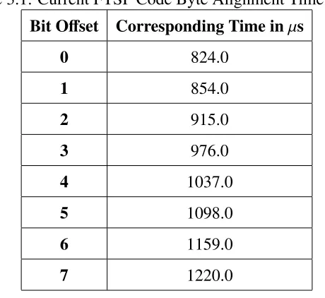
3.1 Current FTSP Code Byte Alignment Time Delay . . . 37
4.1 FTSP paper test parameters and results . . . 43
4.2 Original vs recreated FTSP test parameters and results . . . 44
4.3 FTSP test results . . . 50
4.4 FTSP average test results . . . 51
Appendix A . . . 65
Introduction
During the last decade, the majority of engineering applications and processes have migrated
from wired systems to networks of nodes that are wirelessly connected. This change is largely
due to the wide range of merits that wireless communication offers such as versatility and
scal-ablity. These properties allow the end nodes to be easily added/removed in addition to
accom-modating the deployment of nodes in areas that are difficult for humans to reach. WSN’s are
used in a wide range of applications most of which utilize the mobile nature of the network by
placing the sensor nodes on moving parts. This ad-hoc setup allows for many different network
arrangements that can be made within wireless sensor networks, however, along with these
ad-vantages come added complexities. The unreliable nature of the wireless medium makes it
difficult to provide accurate timing information in situations where time-stamp precision is
critical. Time synchronization is used to obtain the exact time that the sensor sends/receives
data or to calculate the current time of the sensor relative to the rest of the network. The need
for time synchronization is largely because in most WSN applications, data is only as
accu-rate as the time-stamp associated with it. To elaboaccu-rate with an example, a health monitoring
application developed by R.A. Bloomfield et al. [1], proposed a knee measurement system
which utilizes wireless sensor nodes placed at different locations on a patient’s knee to obtain
information on the health of the joint. The test involves basic movements of the joint for the
course of an hour. In order to reconstruct the correct alignment of the joint after the
experi-ment is completed, one must ensure that the gathered data is modeled from all the sensors at
the same time. Otherwise it would not be an accurate depiction of the exercise making the
data unreliable. In scenarios like these and many more, time synchronization becomes a
chal-lenge. More specifically, a synchronization protocol is needed in order to ensure the timely
arrival of packets with their corresponding correct time-stamps. Synchronization protocols are
algorithms that attempt to bridge the gap between the time the packet was sent and the time
it was received. This calculation done by estimating either the sent or received time to match
the other. For example, in the case of the flooding time synchronization protocol (FTSP), the
sender will embed its own time as the global time and the receiver will take its received time as
the local time. The protocol then works to estimate the global time from the local time by
sub-tracting calculated estimates of the errors that a packet encounters during wireless transmission
and reception.
This study shows the steps taken to provide a practical implementation of the flooding time
synchronization protocol. The original FTSP paper by Maroti et al. [2] is used as a basis for
this implementation. The available code is studied and it was discovered that there were many
discrepancies between the current implementation [3] and the characteristics of the FTSP that
were detailed in the original paper. Chapter 2 provides some background on the need of
syn-chronization protocols and the currently used protocols in WSN’s. Section 2.2.2 delivers an
overview of the most widely used wireless synchronization protocols including the flooding
time synchronization protocol. Finally, an argument regarding the integrity of the current
im-plementation [3] is presented and backed by a number of recent studies. Chapter 3 explains
the current implementation [3] and the areas where it is lacking. Chapter 3 also includes a
fully functional FTSP solution equipped with a detailed explanation of the modifications done.
Chapter 4 compares the results of this implementation to what was reported by Maroti et al.
[2] and Chapter 5 concludes the study.
1.1
Contributions
The contribution that this thesis achieves is quite important for the field of wireless sensor
networks. The work done in this study is motivated by the absence of a complete FTSP
im-plementation. In addition, research has shown that the results reported in the original 2004
pro-tocols. This work provides a new implementation that will be available for future researchers
as the new benchmark for the FTSP. Implementation flaws in the current implementation are
addressed and corrected in this thesis and a new hardware calibration step is added to achieve
micro-second accuracy. The comprehensive research conducted on the challenging time
syn-chronization problem in this thesis extends the value of the work done to reach a larger
audi-ence. Researchers, working with WSN applications which require micro-second level
accu-racy, will now have a fully functional FTSP implementation with easily reproducible results at
Literature Review
2.1
Wireless Sensor Networks
With the increase in technological advancements, more emphasis has been put on enhancing
the wireless efficiency of current systems. Specifically speaking, wireless sensor networks have
become the basis under which most new applications are built upon. A wireless sensor network,
as the name suggests, is a collection of sensors, stationary or mobile, that are placed in various
locations connected together over a wireless medium. Applications of wireless sensors extend
from smart home networks, area surveillance to military operations and remote sensing [4].
They are usually placed in areas of interest where measurements are to be taken over a period of
time. Initially, WSNs were used to sense and send physical and/or environmental data in order
to monitor a certain behavior, for example, their use in smart home monitoring and vegetable
greenhouse monitoring [5]. Recent advancements in WSNs have created an added complexity
to the networks. Their uses now extend to military target tracking and surveillance, natural
disaster relief, bio medical health monitoring, object and behavior tracking and automation
and hazardous environment exploration [6,7] to name a few; see Figure 2.1 for more WSN
applications.
Furthermore, wireless sensor networks are being utilized in recent medical advancements
in order to monitor a patient’s health profile remotely by checking the physiological data of
the patient [8]. In the military, WSNs are mostly used for detection of any kind of danger
or threat such as sensing chemical or nuclear attacks and alerting the appropriate channels.
Figure 2.1: Applications of Wireless Sensor Networks [6]
Sensing may also be in the form of visual detection of foreign air crafts for national security
purposes. As for a wireless sensor network’s role in natural disasters, they are mainly used for
prediction purposes by monitoring the environment and making forecasts based on calculations
from sensor readings. This kind of WSN application is often used for forest fire monitoring,
earthquake detection and gathering data to learn more about certain ecosystems. More common
and everyday uses of wireless sensor networks are sensors which monitor public areas such as
malls and create alerts if the security is compromised. In addition, some parking lots employ
sensors which can help detect empty parking spaces in order to reduce traffic congestion [9].
Finally, a more complex yet very useful application of wireless sensors is in interplanetary
exploration and high energy physics [10].
The end nodes of WSNs are characteristically low power devices since they usually consist
of one or more sensors, a processor, memory, a power supply, a radio, and an actuator if needed.
WSNs have little or no infrastructure, therefore they can be classified into two types: structured
to perform monitoring and reporting functions. This type of wireless sensor network has the
advantage of being scalable in size since the nodes are deployed in an ad hoc manner on the
field. Node mobility provides the option of sensor deployment in locations that are hard for
humans to reach. However, this characteristic causes fault detection and troubleshooting to
become more difficult. Structured wireless sensor networks are systems of sensors which are
organized in a pre-planned setting. Although this can reduce uncertainty by having easier
access and lower management cost, the amount of nodes that can be used is limited [6].
One of the main challenges of wireless sensor networks is energy consumption. This issue
is due to the large number of processes that sensor nodes need to perform regularly within
their limited lifetime. Another more debated issue that arises is time synchronization which
is done to ensure that all of the sensor nodes have a common global time [11]. Due to the
nature of events taking place in a wireless sensor network, timing is of utmost importance. The
usefulness and validity of the data received is dependent on the time it was received. One of
the simplest examples of time-synchronization is implementing power-saving techniques for
the sensor nodes. Since these algorithms would require the nodes to switch their radios on/off
depending on a certain time schedule, accurate timing must be established among all nodes in
the network for these techniques to work [12].
The unreliability of the wireless medium poses a major threat network security in WSNs.
The susceptible nature of the wireless communication medium makes it accessible to any
de-vice within the vicinity. This lack of security allows an intruder to easily intercept the signal
within the network and make malicious changes [13]. Finally, although the scalability of WSNs
is considered an advantage, it also introduces stringent constraints on the network that need to
be satisfied in order to realize that characteristic [14].
2.2
The Time Synchronization Problem
Time synchronization was initially an issue that was faced by wired networks way before
wire-less networks and has been studied thoroughly from that angle. The GPS (Global Positioning
System), aimed to provide accurate location and timing information for nodes to solve that
not widely available thereby motivating the development of software based time
synchroniza-tion protocols such as NTP (Network Time Protocol)[15]. These protocols will ensure that the
tasks are ordered and processes are time-stamped by a simple call to the kernel. This
proce-dure confirms that the source of time for all the sensors in the network emerge from the same
clock thereby eliminating any ambiguity that is otherwise faced with wireless networks. GPS
coupled with NTP displayed great results for time synchronization in wired networks which
were in the order of a few microseconds [16].
Due to the nature of wireless sensor networks, it is not possible to replicate the same
solu-tion for the time synchronizasolu-tion problem. The limited hardware and computing capabilities of
wireless sensor networks in addition to network instability introduced by the wireless medium
require the creation of a solution unique to WSNs [17]. Furthermore, the characteristics of
wireless sensor nodes as standalone devices impose added complexity. The nodes are each
equipped with sensors, their own physical clock and a processor. This set-up introduces a
vari-able variance to the system making it difficult to choose a common time [18]. As a result,
time-synchronization protocols are designed in order to minimize the error caused by these
uncertainties. In the next section, the different synchronization protocols will be discussed in
addition to their role in reducing uncertainty in wireless sensor networks.
2.2.1
Time Synchronization in Wireless Sensor Networks
Synchronization protocols can be classified in many ways, for the purposes of this study, they
will be classified by their main features. The most common kinds of synchronization protocols
are listed below:
• Internal synchronization vs external synchronization:
Internal synchronization does not have a global time therefore the aim of the protocol is
to minimize the difference between the nodes. With external synchronization, there is a
global time such as UTC (Universal Time Controller) that is available and used by the
nodes [18].
• Master-slave vs peer-to-peer synchronization:
the other nodes synchronize their clock/time to. With peer-peer synchronization, nodes
can communicate directly with each other and by that removing the risk of the master
node failing [18].
• Sender-to-receiver vs receiver-to-receiver synchronization:
Sender to receiver will calculate the delay based on the difference in time-stamps between
the sender and receiver in addition to the time it takes to propagate. However, receiver
to receiver synchronization eliminates the sender role and thereby all nodes will only
operate as receiving nodes. The time-stamps are calculated based on the difference in
times between two receivers when they get the same message [19].
• Clock correction vs un-tethered clocks:
Due to the difference in characteristics of hardware clocks and crystal oscillators between
nodes, the clock drift issue arises. Some synchronization protocols will perform a certain
clock-correction mechanism to account for that problem [18].
• Probabilistic vs deterministic synchronization:
This refers to the way that the clock offset is measured. With probabilistic
synchroniza-tion, the maximum clock offset is calculated based on a probabilistic guarantee with a
known probability of failure. Deterministic synchronization protocols will have an upper
and lower bound set for the clock offset.[18]
• MAC-layer-based approach vs non-MAC-layer-based approach:
Some synchronization protocols are implemented at the MAC layer and are tightly linked
to the access scheme used in order to perform time-synchronization making it more
ac-curate however not modular. In other protocols which are not at the MAC layer, although
they will not offer the same accuracy as those who are but have the advantage of being
modular [10].
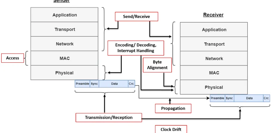
In addition to the attributes discussed, the synchronization protocols are also characterized
by the kinds of errors they help minimize. As shown in Figure 2.2, the main errors faced by
wireless sensor networks are a result of radio message delays. Table 2.1 summarizes the delays
Figure 2.2: Sources of Radio Message Delay
2.2.2
Time Synchronization Protocols for Wireless Sensor Networks
Accurate time synchronization is one of the most debated issues faced by wireless sensor
net-works; therefore, there are many protocols that hope to bridge this gap. In this section, various
kinds of protocols that are being used to synchronize the times of the nodes within a
wire-less network will be discussed. In addition, a comparison will be made using the attributes
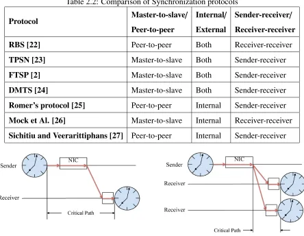
discussed in Section 2.2.1. The initial comparison of the most common time synchronization
protocols for WSNs is done in Tables 2.2 and 2.3 [20, 21]. A more detailed explanation on each
synchronization protocol along with a brief overview of the algorithms used is also provided in
this chapter. Finally, an in-depth study on the Flooding Time Synchronization Protocol (FTSP)
is presented.
Reference Broadcast Time Synchronization (RBS)
The reference broadcast time synchronization protocol is a receiver-receiver based
determin-istic protocol that offers high energy conservation due to its post-facto synchronization [28].
Post-facto synchronization means that the synchronization of the nodes is only done when
necessary. In addition, RBS protocol uses the broadcasting feature of wireless
Table 2.1: Overview of Radio Message Errors Radio Message Delay Comments Error Magnitude for Mica2
Send/Receive
Time for the assembly of the packet to be sent
and signalling to MAC layer/Time for the processing
of received message and signalling to receiving application.
0 - 100 ms
Access Time for packet to access the channel. 10 - 500 ms
Transmission/
Reception
Time for packet to be sent from the first to last bit/
Time for the packet to be received from the first to last bit.
10 - 20 ms
Propagation Time for the packet to travel through air. <1µs
Interrupt Handling
Time incurred from sections in the code disabling interrupts
which are raised from the radio chip to indicate message
transmission or reception to the microprocessor.
5 - 30µs
Encoding/Decoding Time to transform binary data to electromagnetic waves/
Time to transform electromagnetic waves to binary data.
100 - 200
µs
Byte Alignment Delay incurred from bits being received in incorrect order. 0 - 400µs
Clock Drift Delay due to different characteristics of hardware oscillators
making them have different frequencies.
>40µs
of receivers at almost the same time. Similarly to the flooding time synchronization protocol
(FTSP), RBS also exploits this physical property of the wireless medium [18].
Although RBS does not employ MAC layer time-stamping, it can obtain fairly good
ac-curacy because of its receiver-receiver feature. This attribute will allow the elimination of
non-deterministic errors that arise from radio message delivery, such as send and access time,
through reducing the critical path. Figure 2.3 shows how the critical path is reduced by
choos-ing receiver-receiver based synchronization. As illustrated in Figure 2.3, since both receivers
will receive the broadcast message, the difference between their local times can then be taken
in order to estimate the clock offset and correct their times accordingly. Even though RBS
Table 2.2: Comparison of Synchronization protocols
Protocol Master-to-slave/
Peer-to-peer
Internal/ External
Sender-receiver/
Receiver-receiver
RBS [22] Peer-to-peer Both Receiver-receiver
TPSN [23] Master-to-slave Both Sender-receiver
FTSP [2] Master-to-slave Both Sender-receiver
DMTS [24] Master-to-slave Both Sender-receiver
Romer’s protocol [25] Peer-to-peer Internal Sender-receiver
Mock et Al. [26] Master-to-slave Internal Receiver-receiver
Sichitiu and Veerarittiphans [27] Peer-to-peer Internal Sender-receiver
Figure 2.3: Critical path comparison, the sender-receiver critical path (left) and the
receiver-receiver critical path (right) [22]
there is no global time to synchronize to. Although this may reduce cost, it comes at an expense
to the precision of the protocol [18].
Timing-Sync Protocol for Sensor Networks (TPSN)
The timing-sync protocol for sensor networks is a protocol that improved upon the RBS
pro-tocol’s time-stamping weakness. This was achieved by performing MAC layer time-stamping
which resulted in the synchronization error measured for TPSN being reduced by over half than
that of RBS, refer to Table 2.3. TPSN takes a more common sender-receiver approach with
message exchange offering easier handshaking between nodes in order to achieve
Table 2.3: Comparison of Synchronization protocols Cont’d
Protocol Clock
Correction
Probabilistic/ Deterministic
MAC layer/
Standard
Sync
Error
(µs)
RBS [22] No Deterministic Standard 29.1
TPSN [23] Yes Deterministic MAC layer 16.9
FTSP [2] Yes Deterministic MAC layer 1.48
DMTS [24] No Deterministic Standard 32
Romer’s protocol [25] No Deterministic Standard 200
Mock et Al. [26] Yes Deterministic MAC layer 300
Sichitiu and Veerarittiphans [27] Yes Deterministic MAC layer 3000
Prior to the start of this protocol the authors have assumed that the network has a
hierar-chical structure consisting of nodes which are each assigned a certain level (i.e. level i, level
(i+1), ..). This protocol has two main phases:
• Level Discovery phase.
• Synchronization phase.
In the discovery state, a root node is selected and given a label: level 0. The newly elected
root node will then start the synchronization phase by synchronizing each level inode with a
level (i−1) node until they are all synchronized to the level 0 node; the root node [23].
Delay Measurement Time Synchronization Protocol (DMTS)
This sender-receiver algorithm elects a master node which transmits the same synchronization
message to all the receivers at the same time. The master’s time is taken as the global time and
all the receivers will calculate their respective delays from this global time. They will then set
their local time to be the global time plus the delay calculated. The delay that is calculated will
take care of some radio message errors, however, the delay caused by the transmission time,
send/receive times and access time remain. This protocol deals with those two errors in the
• Sender processing time and access time: The protocol will only take a time-stamp when
a clear channel is detected to remove the error caused by those two delays.
• Transmission time: This protocol divides the transmission times into two separate times
since the transmit speeds may be different for each: preamble/start symbols transmission
time and the data transmission time. The delay is then calculated from the speeds of each
part of transmission [24].
Romer’s Protocol
Romer’s protocol was created for time synchronization in Ad Hoc Networks. AD Hoc networks
describe networks in which their nodes are mobile and prone to changes. The protocol does not
work by synchronizing clocks, however, it works on synchronizing time stamps of local clocks
through time transformation. Time synchronization is done by first embedding a time stamp in
the message being sent, and when it is received, the receiver will transform the sender’s
time-stamp to the Coordinated Universal Time (UTC) and finally to the local time of the receiver.
This procedure gives a lower and upper bound on the time stamp in addition to the real-time.
The time taken from the generation of a time stamp at the sender to the reception of it at the
receiver node. The lower and upper bounds of this time are calculated and transformed to the
time of the receiver. The receiver, now equipped with the upper and lower bounds will subtract
this transformed time from the time of arrival which is taken at the reception by the receiver’s
local clock [25].
Mock et Al.
This protocol utilizes the master-to-slave mechanism and extends the IEEE 802.11 standard
where a chosen master will send out a “high-priority” message for all the other “slave” nodes
to synchronize their virtual clocks to. In addition, this protocol is similar to RBS since it too
uses the property of the wireless medium and by that reduces the critical path in the same way.
This is summarized by the following steps:
• All of the nodes (master and slave) then receive the “indication message” and record
their local time stamp at reception.
• The master then sends its time stamp for the last indication message to all the slaves.
• The slave nodes then correct their local clocks based on the difference between the
re-ceived time stamp and the local time stamp.
Mock et al. defined a unique rate-based correction algorithm that provides continuous time
synchronization for applications where message loss can’t be tolerated. Initially, a maximum
value is set on the number of messages that can be lost during transmission, this is labeled as
“OD” or omission degree. The number of time stamp values “n” needed to ensure that not
more than “OD” number of messages are consecutively lost is then calculated, this is given
by:n= OD+1. The protocol then includes the last calculated “n” number of synchronization
messages within the current synchronization message. This procedure will allow the receiver
to synchronize its clock to the master even if a current message loss was detected [26].
Sichitiu and Veerarittiphans Protocol
This protocol works with both the Mini-sync and Tiny-sync algorithms in order to achieve
deterministic clock synchronization. It is characterized by low complexity and computational
power in addition to operating with limited resources. Tiny-sync and Mini-sync are different in
the amount of resources they use; Tiny-sync using considerably less resources than Mini-sync.
They do however share a lot of common features such as the deterministic nature of calculating
the clock offset and their tolerance to message losses. The way the algorithms calculate the
clock offset is by extending the set-valued estimation method. Sichitiu and Veerarittiphans
protocol modifies the set-valued estimation method slightly and relates the processors and local
time of the nodes in a network to each other using the linear equations below:
t1(t)= a12t2(t)+b12,
a12 = a1−a2,
b12 =b1−b2
Where t1(t) and t(2) are functions of the local clock of nodes 1 and 2 respectively and t is
the UTC. Variables ai and bi are the clock drift and offset of the ith node. These equations
provide a data collection algorithm to get data points (at least two) which are then used for
time synchronization. The main three data points needed to set the clock drift and offset are
governed by the inequalities below:
to(t)< a12tb(t)+b12
tr(t)> a12tb(t)+b12
(2.2)
Where to is a probe message sent from node 1 to node 2 and tb is the same probe message
time-stamped at the receiver and returned to the sender (node 1) who then records the time of
reception of this message astr.
Flooding Time Synchronization Protocol (FTSP)
The Flooding Time Synchronization Protocol (FTSP) is a sender-receiver protocol created by
Maroti et al. that achieves micro-second accuracy in multi-hop networks. FTSP’s robustness
and level of precision is considered to be the best when compared to other available protocols
for sensor networks and has been used for time synchronization in a counter sniper
appli-cation [29]. Table 2.3 shows how FTSP’s synchronization precision surpasses all the other
synchronization protocols described with an average reported time synchronization error of a
single-hop case being 1.48µs. FTSP differentiates itself from other protocols with its ability
to create a synchronization point with only one broadcast message and its promise to remove
interrupt jitter through several techniques such as multiple time-stamping [2, 30].
This protocol uses the flooding or broadcasting of the synchronization message (which
in-cludes the root’s time otherwise called the global time) to all nodes and the receiving node
would generate its own local time thereby creating a global-local time pair. This difference
in the times is therefore called the offset for that pair and since the timestamp is embedded in
the synchronization message, overhead is reduced by achieving time synchronization though
one message transmission. Most of the errors that arise from radio message delivery can be
eliminated at the MAC layer time stamping; however, interrupt handling time, encoding/
to reduce. Both the interrupt handling time and the encoding/decoding time are dramatically
reduced through the multiple time stamping technique described in the next section. The byte
alignment time is calculated using the SYNC bytes and linear regression is used to reduce clock
drift as explained in the sections below.
FTSP also extends its protocol to network-wide time synchronization through multi-hop
synchronization using a unique node ID. This feature allows the network to be dynamic and
the synchronization root node to be re-elected whenever needed. The mechanism with which
this protocol elects/re-elects the root is as follows:
1. When a node waits for “ROOT TIMEOUT” number of seconds without receiving a
syn-chronization message, it declares itself to be the root node, this ensures that there is at
least one root in the network after “ROOT TIMEOUT” number of seconds.
2. In order to ensure that there is only one root node in the network (adhering to the
master-slave dynamic),when a node receives a message with a root ID smaller than its own, it
updates the nodes root ID with the one that was just received.
3. Finally, all the nodes with higher root ID will give up their status to the ones with lower
root ID until the lower remains and only one root in the network remains.
4. Every node will then be synchronized to the global time of the node one level higher that
itself [2, 30].
Multiple Time-stamping :The Flooding Time Synchronization Protocol credits its
multi-ple time stamping technique taken at both the sender and receiver for its micro-second accuracy.
Maroti et al. [2, 30] documented that multiple time-stamps (≈6 according to their calculations)
are to be taken at each byte boundary after the SYNC bytes have been sent. The format of the
packets is shown in Figure 2.4. The aforementioned time stamps will then be normalized by
subtracting a certain delta from them which corresponds to the nominal byte transmission time
after which they will be minimized and finally averaged. A more detailed explanation of this
procedure is described below. As indicated in Figure 2.5, t1to t6are to be minimized by
choos-ing the minimum of each two normalized time-stamps startchoos-ing with t0
6being equal to t6. Maroti
Figure 2.4: Packet format
Figure 2.5: Multiple Time-Stamping Technique
the transfer rate of the hardware. The transfer rate indicated in [2] is 38.4 kbps for the Mica2
hardware used and since each cycle will transmit 16 bits (address bits followed by the 8 data
bits)[31] this computes a delta of 417µs [32]. However, in the case of the Mica2, this research
shows that this delta value does not hold due to hardware clock instability, Chapter 3 provides
more insight on this issue. To elaborate on the time-stamping procedure, see the equations
below.
t05= min(t5,t06−∆)
t04= min(t4,t05−∆)
t03= min(t3,t04−∆)
t02= min(t2,t03−∆)
t01= min(t1,t02−∆)
(2.3)
The average of these time stamps is then calculated as follows:
t0avg = P6
i=1t 0 i
6 (2.4)
This final timestamp is then further corrected with the byte alignment and clock drift
Byte Alignment: Byte alignment errors arise from the difference in the order of the sent
and received bytes. FTSP combats this at the receiver by utilizing the synchronization (sync)
bytes in order to indicate the start of the data received. Once the preamble bytes are received
in the listen state, the protocol moves into the synchronization (sync) state where it compares
the incoming bytes to the sync bytes and stores the number of bits it took until the sync bytes
are received, this is called the offset. This value is obtained from the speed of the radio. For
example, at a data rate of 19.2 kbps, the time delay is calculated for a bit offset of 0 to 7 bits to
be 0 to 365µs respectively [2], see Table 2.4. These values are then used as a look-up table to
provide the delay incurred for the bit offset calculated at the receiver.
Table 2.4: Byte Alignment Time Delay at 19.2 kbps
Bit Offset Corresponding Time inµs
0 0
1 52.1
2 104.3
3 156.4
4 208.5
5 260.6
6 312.7
7 364.8
Clock Drift: The implementation of the protocol [3] was done on the Mica2 [33] hardware
motes and because different sensor motes have different clocks, errors resulting from clock drift
are inevitable. FTSP uses linear regression and the method of least squares to calculate clock
drift and correct the timestamp accordingly. The method of least squares is defined by the
following steps:
2.5.
X =
n
P
i=1 xi
n Y =
n
P
i=1 yi
n (2.5)
The next step is to calculate the slope of the line of best fit using these calculated averages
for any new data point. This is used to forecast the upcoming data points and by that reduce
uncertainty. The equation to calculate the slope using this method is shown below:
m=
n
P
i=1
(xi−X)(yi−Y)
n
P
i=1
(xi−X)2
(2.6)
The authors of the paper have indicated that they achieved good results using only 8 data
points. This means that every 8 packets received, the linear regression and method of least
squares is used to recalculate the slope and then use it as a multiple to help predict the upcoming
data. In the case of this protocol, the data points were (time, offset) where offset is the difference
between the local and global times and time is the current local time of the mote. They then
set the slope to be equal to the clock skew and used it to transform the local time to a global
time. This was the mechanism through which FTSP eliminated clock drift. Although the effect
of clock drift might be slower than other phenomena, the Mica2 oscillators introduce drifts of
up to 40µs per second [2, 30].
FTSP in Recent Studies
According to a recent study made by D. Djenouri and M. Bagaa [34] on synchronization
pro-tocols, it was argued that an implementation which truly follows the FTSP guidelines was not
currently available . Furthermore, new and upcoming synchronization protocols are still
com-paring their efficiency to the values that were reported in the original FTSP paper. For example,
Glossy [35] is a synchronization protocol designed to flood the network with the goal of
im-plicit time synchronization. In the 2011 paper explaining the Glossy protocol, the authors and
creators of the protocol compared it to FTSP. They mentioned the synchronization error (in
the microsecond rage) obtained in Maroti et al.’s paper and used it to show how their protocol
Average TimeSync (ATS) [36] is another synchronization protocol created in 2011 which
also uses FTSP as a benchmark in addition to calling it “the defacto standard for time
synchro-nization in WSN”. In their testing they have indicated that they did use the widely available
FTSP TinyOS [37] implementation in addition to testing both protocols in a 3x3 WSN grid
with a synchronization period T=60 s. Since this study argues that the available online code
is not a true translation of the flooding time synchronization protocol, the relevancy of the
previous comparison might be affected.
In 2011, Thomas Kunz and Ereth MCKnight-MacNeil [38] implemented the clock
sam-pling mutual network synchronization (CS-MNS) algorithm in TinyOS on a hardware similar
to the Mica2 and compared its performance to that of the FTSP. It was found that the FTSP
performed rather poorly than otherwise reported in the original paper. Their final results show
that the CS-MNS algorithm had a final synchronization error of 31 µs compared to 61µs for
FTSP. While the authors of [39] attempted to use the TinyOS 2.x [3] implementation to
recre-ate the results in order to compare with their own protocol, they found that while using the
default parameter settings, the available code FTSP was unable to synchronize the nodes in
the network. The faults they have uncovered in the implementation lead to them modifying
the code in order to obtain results which could be comparable to their own. This variation in
the FTSP code is due to its shortcomings and results in possibly different adaptations of the
protocol which may not be a true translation of the algorithm of FTSP.
The Energy-Balanced time Synchronization protocol (EBS) described in [40] uses FTSP
as a benchmark when analyzing the efficiency of the synchronization protocol. The novel time
synchronization protocol introduced in [41] is implemented in TinyOS and resulted in test
re-sults up to 40% better than those of FTSP. In an attempt to improve the FTSP, the authors
in [42] suggest that their changes to the protocol improves battery life by reducing the
num-ber of sent and received frames by 20%. The testing they have done was via simulation on
OMNeT++, which is an object-oriented modular discrete event network simulator and not on
actual hardware.
P.A Sommer [43] indicated a much deliberated issue that affects the accuracy of the current
FTSP implementation. Due to the nature of the synchronization protocol, the nodes in FTSP
implemented currently adds room for error. This error would occur because of a resetting of
the linear regression process in the case that the difference between the actual received time
and the calculated received time exceeds a certain limit. Since the next node will now not
receive a synchronization message from this node that is currently resetting and attempting to
re-establish synchronization, it will declare itself as the root and by that degrade the
perfor-mance of the network. P.A Sommer explains how the current implementation does not account
for errors that result from this scenario which have proven to be detrimental to the accuracy
of the FTSP. In order to ensure that this error is not exhibited in their implementation, the
authors had to fix the root to one specific node and tested the protocol. The average one-hop
synchronization error recorded after this modification was 9.04µs.
F. Wang et al. [44] created the Extensible time synchronization protocol (ETSP) and used
FTSP as a benchmark to compare their protocol’s performance. The authors implemented both
protocols on the SCSC-RFA1 sensor node from Shandong Computer Science Center which
has similar features to the Mica2 [45]. With their FTSP implementation, they achieved a time
synchronization error that ranged from -2 to 5 ticks whereas they reported an average error
of around 1 tick for ETSP for a single-hop network. Since this sensor node uses a 32 kHz
oscillator, a tick in this setting was defined as 31.25 µs [45] giving us a reported error of
-62.5 to 156.3 µs for the FTSP. These results contradict the precision claims of the original
FTSP paper resulting in poor time synchronization performance when tested by F. Wang et al.
causing them to rule in favor of ETSP.
Furthermore, a recent paper claims that the FTSP is in fact a low accuracy algorithm that
is only useful for short-term applications [46]. This claim contradicts the definition of the
FTSP; it has been advertised as a precise synchronization protocol that achieves micro-second
range accuracy. However both [46] and [47] challenge that claim. G. Huang et al. [46] report
that using the FTSP with a one minute re-synchronization rate achieves a 90 µs error. They
then suggest that FTSP is suitable for low accuracy applications such as surveillance whereas
the authors of the FTSP paper have indicated that it has been used in a sensor network-based
counter-sniper system [28]. There appears to be a huge disconnect between the claims of the
authors of the FTSP paper and the current implementation of the protocol: is it or is it not
time-synchronization community seem to side with the latter on that argument and doubt the
accuracy of FTSP whereas others creating their own protocols still use it as the bench mark for
time-synchronization.
In the 2017 paper, F. Gong et al. [48] present a new way of measuring the performance of
the FTSP while comparing it with a real test-bed FTSP implementation. The protocol is tested
on a TelosB hardware unit using the TinyOS version 2.1.2 [3]. As explained in this research,
the TinyOS version 2.1.2 implementation does not implement the true function of the flooding
time synchronization protocol and therefore their results might not be a true representation of
the protocol. L.Li et al. [49] used a different approach to examine the protocol performance,
they obtained results using the network simulator software ns3 (version 3.26). This paper
presents a new protocol which synchronizes time-stamps from the receiver to a reference time
in a reactive fashion called on demand timestamp synchronization framework (OTSF). The
creators of OTSF compare the performance of their novel protocol to that of the FTSP through
ns3 simulations. Their test results vary with the average sleep interval of the radio, this value
ranges from a minimum of 5 s to a maximum of 25 s. Their mean squared error for the
synchronization error of the FTSP simulation showed a best case scenario of 110 µs at the
minimum average sleep interval of 5 s.
The temperature-compensated Kalman based distributed synchronization protocol (TKDS)
is proposed in [50] and tested against FTSP. The authors vary the effective delay in wireless
transmission and observe how that changes the reported skew and offset values. J. Wang et al.
[51] defined the maximum single-hop delay (effective delay) to be equal to the cycle length
of the transmitter. In the case of [50], they set the default value to be 100 µs and offset and
skew values for FTSP were measured accordingly. At that effective delay, the reported FTSP
skew error was 12 parts per million (which is a unit used to measure the timing accuracy of the
crystals in clock oscillators [52]) and an offset of 16µs. Since the experiment ran for 10 mins
or 600 seconds, then the skew would be 10126 ×600= 7.2 ms. The summation of both gives us a
rather poor result for the Flooding time synchronization protocol. In [53], a modified version
of FTSP, FTSP+, is proposed and implemented with TinyOS 2.1.2. The authors aimed to
improve upon the modularity of the FTSP protocol by eliminating MAC layer time-stamping
stack delay. The accuracy of the FTSP+ was then determined by showing the results of their
implementation on hardware similar to the Mica2. It was noted that this 2016 paper used the
values reported by Maroti et al. in the 2004 paper as a benchmark for comparison of their
proposed protocol’s synchronization error results.
This argument raises the question: If the results in the original paper that was published
in 2004 are not repeatable, how is FTSP still being used as a benchmark for all the new and
upcoming synchronization protocols? The fact remains that there isn’t a single complete FTSP
implementation to be used by others highlighting a need for a fully functional widely available
TinyOS FTSP Implementation
3.1
Current Implementation
The implementation currently being set as the official code for the Flooding Time
Synchro-nization Protocol, which is found on GitHub [3], does not translate the algorithm described
by the flooding time synchronization protocol. One of the first issues noticed was the use of
a millisecond clock in the current implementation for time-stamping purposes. In addition,
the implementation does not perform the multiple time-stamping technique which the FTSP
is characterized by. Moreover, seeing as the time-stamps must be taken after each byte
trans-mission or reception, the byte-wise radio must employ its byte-wise radio chip (CC1000 from
Texas Instruments). According to TEP 133 (TinyOS Enhancement Proposals number 133)
[54], which talks about packet-level time synchronization, the time-stamping approach used is
not one intended for the FTSP. The approach they have used is explained below:
• Sender: time-stamp taken at start of transmission and at the end, the delta of the two
times is embedded in the message.
• Receiver: a local time-stamp is taken at receiver and the delta that was embedded in the
transmitted packet is subtracted from it to obtain the time of the receiver with reference
to the transmitter.
Although the previous procedure outlines a time-stamping mechanism, it does not correspond
to the one required to carry out the FTSP. To be able to perform this protocol as instructed, the
following values are required:
• Sender: time-stamps of first six bytes sent after the transmission of SYNC bytes
• Receiver: time-stamps of first six bytes received after the reception of SYNC bytes
In the code segments below, the current implementation of FTSP appears to use a single
time-stamp and by that confirming that multiple time-time-stamping does not take place. The
program-ming language used for the FTSP implementation is nesC (nc). NesC is an extension to the C
programming language created for event-driven programming on the TinyOs platform [55].
This code is taken from the TimeSyncP.nc file in the tinyos-release/tos/lib/ftsp/ repository
found on GitHub [3].
1
2 t a s k v o i d sendMsg ( )
3 {
4 u i n t 3 2 t l o c a l T i m e , g l o b a l T i m e ;
5 6
7 g l o b a l T i m e = l o c a l T i m e = c a l l G l o b a l T i m e . g e t L o c a l T i m e ( ) ;
8 c a l l G l o b a l T i m e . l o c a l 2 G l o b a l (& g l o b a l T i m e ) ; 9
10 i f( n u m E n t r i e s < ENTRY SEND LIMIT && o u t g o i n g M s g−>r o o t I D !=
11 TOS NODE ID ){
12 ++h e a r t B e a t s ;
13 s t a t e &= ˜ STATE SENDING ;
14 }
15 e l s e i f( c a l l Send . s e n d (AM BROADCAST ADDR, &o u t g o i n g M s g B u f f e r ,
16 TIMESYNCMSG LEN , l o c a l T i m e ) != SUCCESS ){
17 s t a t e &= ˜ STATE SENDING ;
18 s i g n a l T i m e S y n c N o t i f y . m s g s e n t ( ) ;
19 }
20 }
This code segment describes what happens when a message is to be sent. A time-stamp is
The interface GlobalTime is defined for this protocol and specifically the call mentioned has
the function of returning the local time of the mote.
In order to find out if the byte-wise time-stamping was implemented, the interrupt which
would be used to trigger the time-stamping event was found in the original code for the CC1000
radio. Specifically, the function below which is found in the file CC1000SendReceiveP.nc
seems to do that job:
void sendNextByte() {
call HplCC1000Spi.writeByte(nextTxByte);
count++;
}
HplCC1000Spi.writeByte(nextTxByte) will write the byte ”nextTxByte” to the CC1000 bus
thereby allowing us to take a time-stamp at around the same time that happens. After careful
research and inspection of the FTSP code available, it was confirmed that this function was
never used to create byte-wise time-stamps thereby making it impossible for the protocol to
work as specified.
3.1.1
Problem Formulation
Concerns regarding the feasibility of micro-second precision synchronization have been raised
on the TinyOS - Help archived online forum [56]. Responses from the authors of the FTSP
pa-per stated that the papa-per uses an older TinyOS 1.x-based implementation that offers
microsecond-precision time-stamping on the Mica2 hardware. However, that implementation has been
phased out and in the current implementation [3], there does not exist a Hardware Interface
Layer (HIL) component providing micro second granularity. Since the protocol promises
mi-crosecond accuracy, it would be impossible to obtain that kind of accuracy using a millisecond
clock to record time-stamps. The code snippet below taken from the current FTSP
implemen-tation shows that the TMilli clock is the current denomination chosen for the time-stamp:
module TestFtspC
uses
{
interface GlobalTime<TMilli>;
interface TimeSyncInfo;
interface Receive;
interface AMSend;
interface Packet;
interface Leds;
interface PacketTimeStamp<TMilli,uint32_t>;
interface Boot;
interface SplitControl as RadioControl;
}
The above FTSP test code is taken from GitHub [3]:tinyos−release/apps/tests/T estFtsp/
Ftsp/T estFtspC.nc. As previously stated, both the GlobalTime interface and the
Packet-Timestamp interface appear to use a TMilli clock. In addition to that, line 71 in the file
TestFTSPC.nc (Appendix A), clearly shows only one timestamp being taken at the receiver:
uint32 t rxT imestamp=callPacketT imeS tamp.timestamp(msgPtr). As for the sender
times-tamp, that is embedded in the packet during the transmission of the packet. Current
im-plementation embeds a single timestamp from the sender taken after the SYNC bytes have
been sent, however that value is not used at the receiver, the TestFTSP application found
online estimates the global time from the local time (received time) using the command:
call GlobalTime.local2Global(&rxTimestamp). This function is defined in the file
tinyos−release/tos/lib/f tsp/T imeS yncP.ncas:
async command error_t GlobalTime.local2Global(uint32_t *time)
{
*time += offsetAverage +
(int32_t)(skew * (int32_t)(*time - localAverage));
}
The variables shown in this function only take into account the clock drift calculations when
estimating the global time. The CalculateConversion() function will convert the local time to
the global time and is called once from within the processMsg() function. ProcessMsg() is a
task that is posted when a packet is received (in the Receive.receive function). The code
de-scribed fails to perform multiple time-stamping thereby eliminating the possibility of carrying
out the FTSP as initially defined.
3.2
Complete FTSP Implementation
3.2.1
Specifications and Software Setup
The authors of the flooding time synchronization protocol tested the protocol on the Mica2
wireless mote from crossbow that runs the TinyOS open source platform. The two main
com-ponents of the mica2 chip are the Atmega128 Atmel micro-processor chip and the Texas
Instru-ments CC1000 byte-wise radio. TinyOS uses the nesC programming language for event-driven
component-based programming that is widely used in embedded systems [55]. Furthermore,
the code is compiled from within the command line interface using the make tool which is
supported by an extensive make system defined for TinyOS which is to be prompted from
within the application directory of the desired code. In addition, a specific “tinyos-tool-chain”
is needed which contains all the packages used in order to compile the code and program the
hardware (also referred to as a mote). This tool-chain is available on the online GitHub [3]
repository: tinyos/tinyos-release version 2.1.2.
It was concluded that the best option was to run TinyOS on the Linux kernel since it is the
most recently supported kernel. For the purpose of this research a virtual machine was created
which ran Linux, Ubuntu 14.04 since it was found that the TinyOS tool-chain worked best on
that edition. Avr-dude is the compiler used for this hardware and the packages which make up
the tinyos-tool-chain are shown below.
• avr-binutils-tinyos.
• avr-libc-tinyos.
• avr-optional-tinyos.
• avr-tinyos-base.
• avrdude-tinyos.
In addition, tinyos-tools and the nesC library must also be downloaded and installed. Finally,
since PC-mote communications are java-based, it is vital to install the Java Development Kit
for mote programming.
The Mica2 radio is rated for 900 MHz however it has a range of frequencies it can be
set to in the make file of each application. It is crucial to set all of the frequencies of the
motes to be the same to allow for radio communication through the following command:
CFLAGS += -DCC1K_DEF_FREQ=900000000. Since this application depends on radio
com-munications from specific nodes, it is important to set the node ID of the mote that can be
done at the time of programming. The MIB510 programming board is used to program the
Mica2 through the commandmake install.0x0002 mica2 mib510,dev/ttyUSB0where
0x0002 is the nodeID and/dev/ttyUSB0 is the port through which the programmer is connected
to. Prior to downloading the program on the mote, it must first be compiled offline using the
“make mica2” command and manually debugged. Testing and debugging are done online using
the hardware since there isn’t an integrated development environment for the Mica2 hardware.
3.2.2
Mica2 Hardware Calibration
Due to the hardware limitations of the Mica2, this step was added to obtain micro-second
accuracy for the synchronization error values. More details on the nature of this limitation
are described in the next section under implementation difficulties. The values that need to be
re-calculated for each Mica2 unit are the byte transmission time (the time it takes to transmit
a byte) and the bit offset time. In order to obtain these values the following procedure was
carried out:
• Record the time-stamps taken after the sync bytes have been sent/received and calculate
time taken for further calculations. The byte transmission time is calculated for the
sender and the receiver as slight differences were noticed that might affect data accuracy.
• The calculated byte transmission time is divided by 8 to get a single bit transmission
time. This value is used to calculate the bit offset time from the bit offset at the receiver.
For a bit offset of 0 the bit offset time is 0 µs, for a bit offset of 1 the bit offset time is
1×(single bit transmission time), for a bit offset of 2 the bit offset time is 2×(single bit
transmission time) and so on until a bit offset of 7. This calculation will populate the
bit offset correction array with the new values that better match the clock of the Mica2
hardware being used. These newly calculated constants will be the values used for the
byte alignment calculations.
3.2.3
Description of Implementation Code
The Flooding Time Synchronization promised to minimize interrupt and software jitter through
its novel multiple time-stamping technique. This research and investigation confirmed that this
technique has not been part of the current online code repository containing the implementation
of the protocol. Consequently, the implementation presented in the following sections alters
the available code by taking into account the FTSP algorithm and the shortcomings described
earlier to perform the desired outcome. The base files used for this are listed below:
• TestFtspC.nc.
• CC1000SendReceiveP.nc.
• CC1000CsmaRadioC.nc.
The files below were created in order to utilize the micro-second clock:
• TimeSyncMicroC.nc.
• MuxAlarmMicro32_.nc.
• MuxAlarmMicro32.nc.
• MuxAlarmMicro16.nc.
• AlarmCounterMicroP.nc.
• HilTimerMicroC.nc.
• TimerMicroC.nc.
• TimerMicroP.nc.
Micro-Second Clock
Given that the HIL component providing TMicro time does not exist, the 32 kHz code was
used as a base for a TMicro implementation. In addition to changing the wiring to use the
newly created TMicro HIL component, all the precision tags used for the interfaces which are
part of the time-stamping process were changed to [TMicro].
Starting with the TestFtspC.nc file, the precision tags in the GlobalTime interface and
PacketTimeStamp interfaces were changed from from TMilli to TMicro. In addition, similar
changes had to be done in the CC1000SendReceiveP.nc file which describes the logic behind
the sending and receiving functions of the CC1000 radio. Currently both the PacketTimeStamp
and LocalTime interfaces in CC1000SendReceiveP.nc are defined for TMilli and T32khz but
not TMicro. In order to use TMicro precision for those interfaces they must be defined in the
CC1000SendReceiveP.nc file. The following definitions were developed:
• async command bool PacketTimeStampMicro.isValid(message_t* msg).
This function will return a boolean value to indicate whether the timestamp of the
mes-sage (msg) is valid or not by performing a check. The same check is done on all
denom-inations (TMilli, T32kHz, TMicro) since the over the air value is always 32 kHz.
• async command uint32_t PacketTimeStampMicro.timestamp(message_t*
msg). Since the value of the timestamp is always in the 32khz precision, in order to
translate it to Micro it must be shifted. In the approach specified, this timestamp will
calculate the offset in 32 kHz, shift it by 5 (offset>> 5) and add it to the current local
• async command void PacketTimeStampMicro.clear(message_t* msg)
Removes current Time-stamp.
• async command void PacketTimeStampMicro.set(message_t* msg,
uint32_t value)
Using the same mechanism of calculating the offset of the timestamp and adding it to the
local time, the setting is done the same way in TMicro then translated to 32 kHz before
being inserted in the metadata of the packet.
The configuration file CC1000CsmaRadioC.nc was also changed by providing the wiring
for the PacketTimeStampMicro interface to the CC1000SendReceiveP.nc. In addition, the
TimeSyncMicroC.nc file had to be created in order to be able to use the defined FTSP TimeSyncP
component with the micro-second granularity. TimeSyncC.nc was used as a template and the
precision was changed to TMicro for all.
However, after careful examination of the ftsp code found in tos/lib/ftsp, changing the
pre-cision of the current time-stamping code still does not reflect the flooding time synchronization
protocol algorithm therefore the packet time-stamping has to be done from scratch. This issue
is explained further in the multiple time-stamping code section. Nevertheless, obtaining the
Local Time in TMicro is needed in order to carry on with the time-stamping. That step is done
by creating the following components:
components CounterMicro32C, new CounterToLocalTimeC(TMicro) as
CounterToLocalTimeMicroC;
After which they are then wired to give us LocalTimeMicro for the CC1000SendReceiveP.nc
file:
CounterToLocalTimeMicroC.Counter -> CounterMicro32C;
SendReceive.LocalTimeMicro -> CounterToLocalTimeMicroC;
The HilTimerMicroC file created describes a microsecond timer for the Mica2 that is built
upon a hardware timer. The interfaces provided areInit,Timer<TMicro> as
TimerMicro[uint8_t num]and LocalTime<TMicro>. The implementation is shown
be-low:
2
3 enum {
4 TIMER COUNT = u n i q u e C o u n t ( UQ TIMER MICRO )
5 }; 6
7 c o m p o n e n t s A l a r m C o u n t e r M i c r o P , new AlarmToTimerC ( TMicro ) ,
8 new V i r t u a l i z e T i m e r C ( TMicro , TIMER COUNT ) ,
9 new C o u n t e r T o L o c a l T i m e C ( TMicro ) ;
10
11 I n i t = A l a r m C o u n t e r M i c r o P ; 12
13 T i m e r M i c r o = V i r t u a l i z e T i m e r C ;
14 V i r t u a l i z e T i m e r C . TimerFrom −> AlarmToTimerC ;
15 AlarmToTimerC . Alarm −> A l a r m C o u n t e r M i c r o P ;
16
17 L o c a l T i m e = C o u n t e r T o L o c a l T i m e C ;
18 C o u n t e r T o L o c a l T i m e C . C o u n t e r −> A l a r m C o u n t e r M i c r o P ; 19 }
TEP 102 [54] describes how the timers are chosen, it states that “a new timer is allocated
using unique(U Q T I MER MILLI) to obtain a new unique timer number,” has been changed
to U Q T I MER MICROfor this study. They explained how the timer will then be “used to
index the TimerMilli parameterised interface.” In the case of this thesis, it is the TimerMicro
interface. The header file Timer.h definesU Q T I MER MICRO which has been used in the
newly created TimerMicroC and HilTimerMicroC files. TimerMicroC.nc and TimerMicroP.nc
files were both created.
Since the HilTimerMicroC depends on an AlarmCounterMicroP component, it had to be
created. The AlarmCounterMicroP.nc file configures the hardware timer for use as the Mica2’s
microsecond timer with the AlarmCounterMicroC.nc being the wiring file created for it.
Finally, a TimerMicroP.nc file was created outlining the configuration of virtualized
mi-crosecond timers which auto-wire the timer implementation (TimerC) to the boot sequence
and export the various Timer interfaces. TimerMicroC.nc was then added to create the
ab-straction for this timer in the form of a component which is instantiated in order to give an
Multiple Time-stamping Code
The multiple time-stamping is done on a byte-by-byte basis at the sender and receiver in
the CC1000SendReceiveP.nc file. The function used to obtain the time is the
LocalTimeMi-cro.get() that was discussed earlier. A counter was created in order to hold the number of bytes
sent after the sync bytes have been sent, lets call that txcount. Similarly the receiver also had a
counter which held the number of bytes received after the sync byte has been received, this is
labelled rxcount. These respective tx/rx counters are set after the SYNC byte is transmitted/
re-ceived and the number of bytes sent after the SYNC byte is then calculated using a difference
of the local rx/tx count (which remains constant throughout the packet) and the packet count
(which is incremented after each byte transmission or reception throughout the packet). Both
the packet counter and the local tx/rx counters are reset for a new packet. Using this difference,
the first six bytes that are sent/received are time-stamped and their time-stamps are recorded.
The values of the time-stamps are then used in order to obtain t0, which as explained in
Equa-tion (2.3), is the minimum of the last received timestamp minus the byte transmission time and
the current received timestamp. The byte transmission time for the hardware was calculated
using the procedure detailed in Section 3.2.2, this produced a value of 378 ticks for the sender
and 384 for the receiver. The time-stamps are recorded first and then compared to each other
starting with the last timestamp until the first one with the results of that comparison being
held in a new variable. The average of these minimized normalized time-stamps is then taken
and embedded into the sender/receiver before the packet is finished transmitting/receiving. The
pseudo code used for the data transmission is shown below:
1 v o i d t x D a t a ( ) { 2
3 s e n d N e x t B y t e ( ) ;
4
5 i f ( n e x t T x B y t e == SYNC BYTE2 ) {
6 / / SYNC WORD h a s j u s t b e e n s e n t
7 t x C o u n t = c o u n t ;
8 } 9
![Figure 2.1: Applications of Wireless Sensor Networks [6]](https://thumb-us.123doks.com/thumbv2/123dok_us/1929350.1253359/13.612.95.540.72.349/figure-applications-of-wireless-sensor-networks.webp)


![Table 4.1: Original FTSP paper test parameters and results [2]](https://thumb-us.123doks.com/thumbv2/123dok_us/1929350.1253359/51.612.90.549.86.405/table-original-ftsp-paper-test-parameters-results.webp)

