Combination of various data analysis techniques for efficient track reconstruction in very high multiplicity events

Combination of various data analysis techniques

for efficient track reconstruction in very high multiplicity events

FerencSiklér1,a

1_{Wigner RCP, Budapest, Hungary}

Abstract. A novel combination of established data analysis techniques for reconstructing

charged-particles in high energy collisions is proposed. It uses all information available in a collision event while keeping competing choices open as long as possible. Suitable track candidates are selected by transforming measured hits to a binned, three- or four-dimensional, track parameter space. It is accomplished by the use of templates taking advantage of the translational and rotational symmetries of the detectors. Track candi-dates and their corresponding hits, the nodes, form a usually highly connected network, a bipartite graph, where we allow for multiple hit to track assignments, edges. In order to get a manageable problem, the graph is cut into very many minigraphs by removing a few of its vulnerable components, edges and nodes. Finally the hits are distributed among the track candidates by exploring a deterministic decision tree. A depth-limited search is performed maximizing the number of hits on tracks, and minimizing the sum of track-fitχ2_{. Simplified but realistic models of LHC silicon trackers including the relevant}

physics processes are used to test and study the performance (efficiency, purity, timing) of the proposed method in the case of single or many simultaneous proton-proton collisions (high pileup), and for single heavy-ion collisions at the highest available energies.

1 Introduction

Traditional methods of track reconstruction can be scaled to work in high multiplicity events, namely in many simultaneous collisions (pileup) of elementary particles [1, 2] and in high multiplicity single heavy-ion collisions. Nevertheless the performances are not optimal, efficiency and purity are reduced, especially at low momentum. That is why present data taking conditions and further luminosity and energy upgrades of high energy particle colliders, as well as those of detector systems, call for new ideas.

Image transformation methods and neural networks [3] are often used in gas detectors (time pro-jection chambers [4, 5] and transition radiation trackers [6, 7]). In the case of silicon trackers the com-binatorial track finding methods employed for trajectory building mostly use local information [8, 9]. They start with a trajectory seed and build a trajectory by extending the seed through the detector lay-ers, picking up compatible hits. In the case of very many compatible hits the number of concurrently built trajectory candidates must be limited. Only some of the best candidates are kept which biases the final result. In this sense decisions are made too early. In addition, trajectories are mostly treated separately, there is no interaction between their assigned hits.

In this study a combination of established data analysis techniques for charged-particle recon-struction is proposed. It uses all information available in an event while keeping competing choices open as long as possible.

2 Silicon detectors at particle colliders

At currently operating particle colliders the interaction region is very narrow (of the order of 50μm) in bothxandy(transverse) directions, while inz(longitudinal or beam) direction it is long, with a characteristic size of about 10 cm [10]. For single heavy-ion collisions thez0position of the primary

interaction (vertex) is estimated with good precision using the copiously produced highpTparticles,

thanks to the small pointing uncertainty of their tracks, reconstructed with traditional methods. In the case of single or multiple pp collisions no such information on the locations of the interaction vertices exists.

The trajectory of a primary particle is primarily determined by its initial position (0,0,z0) and

parameters (q, η,pT, φ0) of its initial momentum at creation. Hereqis the charge,η=−ln tan(θ0/2) is

the pseudorapidity,pTis the transverse momentum,φ0andθ0are the azimuthal and polar angle of the

initial momentum vector in spherical coordinates. In a large volume solenoid the magnetic field near the center of the detector is rather homogeneous and points in thezdirection. Hence in small volumes the trajectories of charged particles can be approximated by piecewise helices. For practical purposes a primary particle is parametrized by (kT,sinhη, φ0,z0) in the following, wherekT =q/Ris the signed

curvature of the projection of its trajectory on the transverse (bending) plane,Ris its radius. If the particle is singly charged the curvature is connected topTaspT=eBzR, whereeis the electric charge

of a proton.

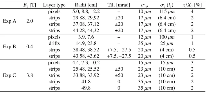
Silicon trackers generally consist of several concentric cylindrical layers. Those close to the nom-inal interaction point are equipped with tiny pixel sensors, while others contain long strip sensors. Some strip layers are double-sided, they are located very close to each other two by two, and have a small relative tilt angle. The main characteristics of the inner barrel silicon detectors of the studied experimental setups are given in Table 1.

The trajectory of the primary particle intersects the concentric cylindrical layers and leaves hits behind in the silicon (Fig. 1). In the simplified case, when the magnetic field is homogeneous and if

Table 1.The main characteristics of the inner barrel silicon detectors of the studied experimental setups.

Bz[T] Layer type Radii [cm] Tilt [mrad] σrφ σz(lz) x/X0[%]

Exp A 2.0

pixels 5.0, 8.8, 12.2 – 10μm 115μm 4 strips 29.88, 29,92 ±20 17μm (6.4 cm) 2 strips 37.08, 37,12 ±20 17μm (6.4 cm) 2 strips 44.28, 44,32 ±20 17μm (6.4 cm) 2

Exp B 0.4

pixels 3.9, 7.6 – 12μm 100μm 1

drifts 14.9, 23.8 – 35μm 25μm 1

strips 38.48, 38.52 +7.5,−27.5 20μm (4 cm) 0.5 strips 43.58, 43.62 +7.5,−27.5 20μm (4 cm) 0.5

Exp C 3.8

pixels 4.4, 7.3, 10.2 – 15μm 15μm 3

strips 25.48, 25,52 ±50 23μm (10 cm) 2 strips 33.88, 33.92 ±50 23μm (10 cm) 2

strips 41.8 0 35μm (10 cm) 2

-40 -20

0 20

40 -80-60

-40-200 204060

80 -40

-20 0 20 40

y

[cm]

Exp B

x[cm] z[cm]

y

[cm]

-40 -20

0 20

40 -80-60

-40-200 204060

80 -40

-20 0 20 40

y

[cm]

Exp C

x[cm] z[cm]

y

[cm]

Figure 1.Left: Pixel hits (red open squares) and strip hits (red solid sections) of a single inelastic pp collision

from simulation of Exp B. The location of the primary interaction is plotted with a green circle, the beam-line is indicated by a gray straight line. Charged particle trajectories (blue dashed curves) are also plotted. Right: Event with 40 simultaneous inelastic pp collisions from simulation of Exp C.

the detector material and its physical effects are neglected, the position of those hits could be precisely determined by simple equations. The physical effects of detector material changes this overly simple picture.

2.1 Physical effects

When a long lived charged particle propagates through material the most important effects which alter its momentum vector are multiple scattering and energy loss. The distribution of multiple Coulomb scattering is roughly Gaussian [11], the standard deviation of the planar scattering angle is

θ0=

13.6 MeV

βcp z

x/X01+0.038 ln(x/X0), (1)

wherep,βc, andzare the momentum, velocity, and charge of the particle in electron charge units, andx/X0is the thickness of the scattering material in radiation lengths. Momentum and energy is lost

during traversal of sensitive detector layers and support structures. To a good approximation the most probable energy lossΔ_p, and the full width of the energy loss distribution at half maximumΓ_Δ[12] are

Δp=ξ

ln2mc

2_β2_γ2_ξ

I2 +0.2000−β 2_−δ

, ΓΔ=4.018ξ, (2)

whereξ = K₂z2Z

Aρβx2 is the Landau parameter; K = 4πNAr2emec2; mis the mass of the particle; Z,

2.2 Hit clusters

An incoming charged particle loses energy in the sensitive detector elements by producing electron-hole pairs. The neighboring channels collecting a charge above a given threshold are grouped to form a cluster, a reconstructed hit. The size (dimensions) of the cluster depends on the angle of incidence of the particle: bigger angles will result in larger clusters. Due to the large fluctuations in energy loss, the measuredwrφ andwzdimensions of the clusters will differ from the expected ones. In order to

model these effects in the simulation, the cluster dimensions are varied by one unit in both directions for pixels, and up and down by two units in rφ direction for strips. In addition, if the size of a pixel cluster is at least two units in both directions, the layout of pixels with charge deposit and its location relative to the nominal interaction point usually indicate the sign of the electric charge of the particle. This way a pixel cluster is characterized by the measured widthswrφandwz(dimensions of

its rectangular envelope), and the charge, which can be±1 or left unknown. A strip cluster has only one such quantity, itswrφwidth.

2.3 Particle tracking

The Kalman filter is widely used in particle physics experiments for charged track and vertex finding and fitting and provides a coherent framework to handle known physical effects and measurement uncertainties [13]. It is equivalent to a global linear least-squares fit which takes into account all correlations coming from process noise. It is the optimum solution since it minimizes the mean square estimation error.

The state vectorx=(k, θ, ψ,rφ,z) is five dimensional, consisting of the signed inverse momentum, local polar angle, local azimuthal angle, global azimuthal position, and global longitudinal position, respectively. The propagation function f(x) from layer to layer is calculated analytically using a helix model. Multiple scattering and energy loss in tracker layers is implemented with their Gaussian approximations shown in Eqs. (1)–(2). The propagation matrixF=∂f/∂xis obtained by numerical derivation. The measurement vector for pixel hitsm = (rφ,z) is two dimensional, for strip hits

m = (rφ) it is one dimensional. The covariance of the process noise isQ = (Fk⊗FT_k)σ2_k +(Fθ⊗ FT

θ)σ2θ+(Fψ ⊗FψT)σ2ψ, whereσk =kσΔ/β,σθ = σψ = θ0andFa =∂f/∂xa is a vector. Multiple

scattering contributes both to the variation ofθandψ, while energy loss affects onlyk. The covariance of measurement noiseVis a function ofσ2_rφandσ2_z, with slightly differing form for pixels and strips, where this latter also incorporates the value of the tilt angle.

Simulated particles are tracked while they are in the volume of the tracker detector, that is, trajec-tories looping in the magnetic field are properly followed. In the case of pattern recognition and track reconstruction only inside out propagation is considered.

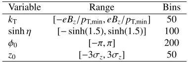
Table 2.Ranges and the optimized number of bins (working point) corresponding to track parameters. The

value ofpT,minis 0.1 GeV/c.

Variable Range Bins

kT [−eBz/pT,min,eBz/pT,min] 50

sinhη [−sinh(1.5),sinh(1.5)] 100

φ0 [−π, π] 200

3 Pattern recognition

Our goal is to collect as much information as possible about potential track candidates, based on the location and shape of the measured hits in an event. To accomplish this, the position of each hit is transformed to a four-dimensional (kT,sinhη, φ0,z0) accumulator space of track parameters. The

ac-cumulator space is not continuous but binned. (Bins are consecutive, adjacent, non-overlapping equal size intervals of a variable.) Ranges and the optimized number of bins corresponding to track parame-ters are shown in Table 2. The transformation is a variant of the well known Hough transform [14]. In the absence of physical effects (Sec. 2.1) the image of a point-like (rφ,z) hit would be a well-defined two-dimensional manifold in that space, while the image of a section-shaped strip hit would be a three-dimensional manifold.

3.1 Preparation of templates

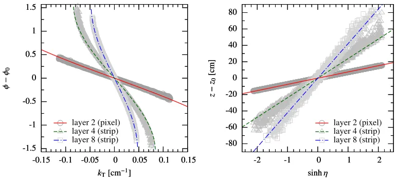
The detector models studied here have translational symmetry in longitudinal (z) and rotational sym-metry in azimuthal (rφ) direction. Theφ−φ0angular difference primarily depends onkT, while the z−z0longitudinal difference is mostly a function of sinhη(Fig. 2). These difference distributions

fur-ther depend on the shape of the hit cluster (Sec. 2.2). For particles with a given (kT,sinhη) and mass,

the (φ−φ0,z−z0) values on a given detector layer populate a small rectangular area. The dimensions

of that area result from the binning of the track parameters.

With help of numerous simulated particles we determine the populated area with help of local linear approximations around the center of each (kT,sinhη) bin. In practice the central values and the

Jacobian is deduced for each bin. The set of these values will be referred to as templates in the fol-lowing. In order to have uniform coverage in all bins, the distribution of simulated particles is chosen

-1.5 -1 -0.5 0 0.5 1 1.5

-0.15 -0.1 -0.05 0 0.05 0.1 0.15

φ

−

φ0

kT[cm−1]

-1.5 -1 -0.5 0 0.5 1 1.5

-0.15 -0.1 -0.05 0 0.05 0.1 0.15

φ

−

φ0

kT[cm−1]

layer 2 (pixel) layer 4 (strip)

layer 8 (strip) _-80

-60 -40 -20 0 20 40 60 80

-2 -1 0 1 2

z

−

z0

[cm]

sinhη -80

-60 -40 -20 0 20 40 60 80

-2 -1 0 1 2

z

−

z0

[cm]

sinhη

layer 2 (pixel) layer 4 (strip) layer 8 (strip)

Figure 2.Left: Distributions ofφ−φ0differences of the hit and track azimuth angles as a function ofkTfor some

selected detector layers. Right: Distributions ofz−z0differences of the hit and track longitudinal coordinates as

a function of sinhηfor some selected detector layers. Values from simulation of Exp C are plotted with various symbols, while the oversimplified expectationsφ−φ0≈ −arcsin(r/2·kT) andz−z0≈2 sinhη·arcsin(r/2·kT)/kT

to be constant inkT, sinhη, andφ0. To limit fluctuations, normal distributed random variables, used

in the simulation of physics processes (Sec. 2.1), are limited to values within 3.5 standard deviations (only about 0.05% lies outside this range). Altogether 2×106pions are generated.

The prepared templates are used in two ways. During the early stage of image transformation they provide a (φ0,z0) accumulator area to increment for each (pixel) hit, in the case of a given (kT,sinhη)

bin. Later they are used to specify a search rectangle on the (rφ,z) plane of a (strip) layer for a given (kT,sinhη, φ0,z0) bin.

Although detector models with only barrel silicon detectors are studied here, the above consid-erations can be adopted to other geometries, such as disks perpendicular to the beam axis. In that case, the translational symmetry would be lost and the templates would become more complex by introducing another dimension, namely the relativezposition of the primary interaction with respect to the longitudinal coordinate of the disk.

3.2 Image transformation

The transformation of spatial information to track space proceeds as described in the following. First hits on the three innermost layers are dealt with, containing exclusively pixel hits. For each a hit all potential (kT,sinhη) accumulator bins are examined and the corresponding possible (φ0,z0) values,

enveloped by rectangles, are determined. Bins within such (kT,sinhη, φ0,z0) area are incremented.

Since we look for tracks with hits on all three innermost layers, only those accumulator bins are kept which gathered votes from all three layers.

The subsequent layers usually contain strip hits. The method used for the innermost layers would not be efficient here because there are far too many accumulator bins to handle. To this end, the kept accumulator bins are examined, corresponding to proto-tracks with three counts, obtained in the previous step. Using the bin coordinates (kT,sinhη, φ0,z0) we look for compatible hits by determining

a search rectangle on the (rφ,z) plane for each layer. For quick access, and in order to facilitate hit selection, strip hits are in advance partitioned on an equidistant grid using their (rφ,z) coordinates.

The search for compatible hits proceeds outwards. It is advantageous since the process can be abandoned if some layers provided no compatible hits while they are still reachable according to the curvature range of the examined bin. In other words, the number of layers with compatible hits should not be very different from the number of reachable layers. (We can allow for a few layers without hits.)

3.3 Trajectory building

Track candidates are built using hits collected in given accumulator bins. Trajectory propagation and track fitting is performed by the extended classical Kalman filter [13] including prediction, filtering, and smoothing, with pion mass assumption. The initial state vector is estimated by placing a helix to the innermost two hits and using the beam-line as a constraint by adding a zeroth point with value

rφ = 0, and with an uncertainty ofσrφ ≈ 50μm. In the case of an off-centered beam,σrφ can be

increased to properly contain the interaction region in the transverse plane.

Trajectory building normally proceeds from inside out and considers all hit combinations recur-sively by forming branches. At each layer there are usually multiple hits to add to the existing tra-jectory. The number of hits to be considered is especially large for the inner strip layers that would exponentially increase the number of trajectory branches.

-40 -30

-20 -10

0

10 -30 -20

-10 0

10

-10 0 10 20 30

y

[cm]

x[cm] z[cm]

y

[cm]

-40 -30

-20 -10

0

10 -30 -20

-10 0

10

-10 0 10

y

[cm]

x[cm] z[cm]

y

[cm]

Figure 3. Hits (red boxes and line sections) belonging to a given bin in the accumulator space and trajectories

propagated to the outermost detector layer (blue dashed curves). The beamline is indicated with the gray line.

already have a good knowledge about the parameters of the track that is being reconstructed. Instead of going to the next (strip) layer, the trajectory is at once propagated to one of the potential hits in the outermost detector layer (Fig. 3). During propagation the physical effects of the crossed layers are duly taken into account, but information about their hits is not used. The outliers in the inter-mittent omitted layers are detected next in the smoothing step of the deficient trajectories using the smoothed residual [13]. Those (strip) hits in the upper 0.5% tail of the correspondingχ2_distribution

are discarded.

Once the list of compatible strip hits is narrowed down, full trajectory building with the selected hits is performed again. During trajectory building we can allow for a few (one or two) missing hits. It may mean no hit at all or the case whenχ2 _{is too large for a given number of degrees of freedom}

(ndf). If there are too many missing hits, the process is abandoned. In order not to lose a noticeable amount of track candidates, but also to have a good selection power, trajectories in the upper 0.5% tail of the correspondingχ2distribution are discarded and not developed further.

4 Optimal distribution of hits among tracks

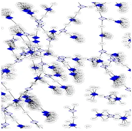
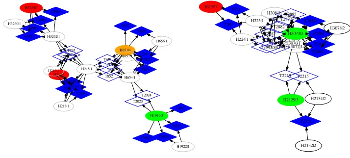
In the end we have a set of track candidates with the somewhat unusual property that temporarily several track candidates may share some hits. Our goal is to resolve these ambiguities, hit confusion, by optimally allocating the hits among tracks, since all hits must be assigned to not more than one track. The hits and track candidates, and their relations, are best represented by a bipartite graphG. The nodes ofGare from two disjoint sets: hits and track candidates, such that each edge connects a hit to a track candidate (Fig. 4). Our goal is to assign all hits to at most one track, while keeping an eye on the total merit of all tracks (χ2_{) in the event.}

H2452|1 T95 T5107 H2453|1 T3740 H2454|1 H2455|1 H2456|1 H2457|1 H2458|1 H2459|1 H2460|1 T1234 H4814|1 H4815|1 H4816|1 H4820|1 H3197|1 T163 T7225 H3198|1 T6669 H3199|1 H3200|1 H3201|1 H3202|1 H3203|1 H3204|1 H3205|1 H3016|1 T5401 1 019|1 0|1 3021|1 H3022|1 H6272|1 T811 T5589 H6273|1 H6274|1 H6275|1 H6276|1 H6277|1H6278|1 H6279|1 H6280|1 T3342 6225 4|1 T4358 06 |1 H8582|1 H3699|1 T1069H3700|1 H3701|1 H3702|1 H3703|1 H3704|1 H3705|1 T1781 H3706|1 H3707|1 H2052|1 T1213 T H6484|1T1219T1223

T6228 H6485|1 H6487|1 H6488|1 H4902|1 H4903|1 H6486|1 H8240|1 T1243 T6042 H8241|1 H8242|1 H8243|1 H8244|1 H8245|1 H8246|1 H8248|1 H8247|1 H3894|1 T1332 T6758 H3895|1 H3896|1 H3897|1 H3898|1 H3899|1 H3900|1 H3901|1 H3902|1 H2389|1 T1536H2390|1 H3805|1 T1546 H3806|1 H3807|1 H3810|1 H3811|1 H3812|1 H3813|1 H3808|1 H3809|1 T5622 H570|1 T1757 H6302|1 H8599|1 T4924 H8600|1 H7001|1 T1769H7002|1 H7003|1 T7005 H7004|1 T1777 H7005|1 H7006|1 H7007|1 H597|1 T1786T4925 H976|1 T1825T4510 H4640|1 T3651 H7570|1 T1946 1 1 H595|1H596|1 H598|1 H599|1 H600|1 H601|1 H602|1H603|1 H975|1 H977|1 H978|1 H979|1 H980|1H981|1 H982|1 H983|1 H677|1 T1916 T4979 H678|1 H679|1 H680|1 H681|1 H682|1 H683|1 H684|1 H685|1 H686|1 T1936 H687|1 H688|1 H689|1 H690|1 H691|1 H692|1 H693|1 H694|1 H7565|1 H7566|1 H7567|1 H7568|1 H7569|1 H7571|1 H7572|1 H7573|1 4|1 T H13 H1355|1H1 H1357|1 H1358|1 H1360|1 H3314|1 T2320 T3880 H7635|1T2329 H7636|1H7637|1 T6280 H7638|1 H7639|1 H7640|1 H7641|1 H7642|1 H993|1 T2409 H994|1 H995|1 H996|1 H997|1 H998|1 H999|1 H1000|1 H8249|1 T2540 H8250|1 H8251|1 H8252|1 H8253|1 H8254|1 H8255|1 H8256|1 H7141|1 T2577 H7142|1 T3889 T4139 H7143|1 H7144|1 H7145|1 H7146|1 H7147|1 H7148|1 H7149|1 H6966 T3702 H6967|1 H6908|1 T2727 H6910|1 H6911|1 H6912|1 H6913|1 H6914|1 H6915|1 H6916|1 5356 1 T2915 H1512|1 H1517|1 H1518|1 H7547|1 T3016 H7548|1 H7549|1 |1 H7551|1 H7552|1 H7553|1 H7554|1 H7555|1 H5041|1 T3151 H5042|1 H5043|1 H5044|1 H5045|1 H5046|1 H5047|1 H5048|1 H5049|1 T3822 H6119|1 H4641|1 H4642|1 H4643|1 H4644|1 H4645|1 H4646|1 H4647|1 H4648|1 H6968|1 H6969|1 T6430 H6970|1 H6971|1 H6972|1 H6055|1 H6056|1 T5619 H6057|1 H3307|1 H3308|1 H3309|1 H3310|1 H3311|1 H3312|1 H3313|1 H3315|1 H3830|1 T4131 H3835|1 T3988 H7677|1 T3997 H7678|1 H7679|1 H7680|1 H7681|1 H7682|1 H7683|1 H7684|1 H3717|1 T4028 H3718|1 H3719|1 H3720|1 H3721|1H3722|1 H3723|1 H3724|1 H3725|1 H7747|1 T4050 H7748|1 H7749|1 T6556 H7750|1 H7751|1 H7752|1 H7753|1 H7414|1 T4076 H7415|1 H7416|1 T6797 T7244 H3828|1 H3829|1 H3831|1H3832|1 H3833|1 H3834|1 H3836|1 H5637|1 T7198 H6007|1 T4354 T7275 H6008|1 H7345|1 T5565 H6077|1 H6078|1 H103|1 T4500 H104|1 H105|1 H106|1 H107|1 H108|1 H109|1 H1326|1 T4862 H3617|1 H3618|1 H3619|1 H3621|1 H3622|1 H3623|1 H3624|1 H3944|1 T4878 H4141|1 T7009H6901|1 T5000 H8587|1 H668|1 T4963 T6167 H669|1 H670|1 H671|1 H672|1 H673|1 H674|1 H6899|1 H6900|1 H6902|1 H6903|1 H6904|1 H6905|1 H6906|1 H6907|1 H7814|1 H7815|1 H8490|1 H1586|1 T5437 H1587|1 H1588|1 H1589|1 H1590|1 H1591|1 H1592|1 H1593|1 H1594|1 H7346|1 H7347|1H7348|1 7349|1 H7350|1 51|1 H7352|1 H7353|1 H6852|1 H2393|1 H3031|1 H4142|1 H4143|1 H3986|1 T5657 H3987|1 H3988|1 H3989|1 H3990|1 H3991|1 T6694 H3992|1 39|1 H137|1 90|1 H2377|1 H575|1 H4021|1 H8031|1 T6434 H8032|1 H8033|1 H8034|1 H8035|1 H6541|1 T6464 H6542|1 H6543|1 H6544|1 H6545|1 H6546|1 H6547|1 H6548|1 H6549|1 H5163|1 T6524 H5164|1 H5165|1 H5166|1 H5167|1 H5168|1 H5169|1 H6006|1 6|1 7587|1 H2374|1 H5638|1 H5639|1 H5640|1 H5641|1 H5642|1 H5643|1 H5644|1

Figure 4.A small fraction of the bipartite graphGof hits (ellipses) and track candidates (blue diamonds) for a

multiple pp collision event (40 simultaneous inelastic pp collisions). Directed arrows, graph edges, show potential hits-to-track candidate assignments.

n=9), and their corresponding hits. Thanks to the high number of hits required, these track candidates are likely real. Selected tracks are again stored, nodes and edges removed fromGas above. Then the process is restarted with the subgraph of track candidates withn−1 hits, iterating down to the subgraph of track candidates with three hits.

4.1 Disconnecting a subgraph

The graphs encountered are usually highly connected. If we would try to allocate the hits to tracks one by one, the number of trials needed would explode exponentially with increasing number of nodes. In order to reduce the complexity of the problem the graphs should be partitioned into several small pieces. This can be accomplished by finding vulnerable components in the graph whose removal disconnects the graph. Such vulnerable elements are special edges (bridges) and special nodes (artic-ulation points) whose deletion increases the number of connected components of the graph. Of course this way some tracks would lose a hit, but that is only a small price to pay.

H210|6

T283 T293 T294

T295 T297 T298

T299 H215|1

T849

T850 T851

T852 H217|1

H218|1 H3262|1 T2981

T2990 T2991

T2992

H651|4 T841

T853 T855 T856 T857

H654|1

T2023 T2024

H656|1

H657|1

H1919|3 T865

T2022 T2025

T2029 H1922|1 H3254|7

H3260|1

H219|7

T301 T311

H224|1 T2879 T2881 T2887 H225|1 T2877

T2882

T2883 T2885

H2129|3

T2212 T2215 T2219

H2132|2 H2134|2 H3077|1 T2438

T2884

T2888 T2890

H3076|1 H3073|3

H3078|2 H3081|1

Figure 5.Example minigraphs obtained after the removal of all bridges and articulation points from the bipartite

graphGof hits and track candidates, in the case of a multiple pp collision event (40 simultaneous inelastic pp collisions). The colors of contracted hits (ellipses) refer the number of hits with identical role (red – 6 or more, orange – 4 or 5, green – 3, white – 1 or 2). Filled track candidates (blue diamonds) indicate true tracks, while the others (open diamonds) show candidates where one or more hits are not in place.

process new vulnerable elements may come to light, hence the disconnecting steps are repeated until no new such elements are found.

In addition, the resulted graph is further partitioned into disjoint graphs. This task is best accom-plished by the flood fill method embedded into the above detailed traversal technique. The output of the disconnecting step is a large set of disjoint minigraphs.

In high-pileup pp collision events there are usually several thousand track candidates. Their corre-sponding bipartite graphGand its subgraphs contain several hundred bridges and up to 50 articulation points. Once the subgraphs are disconnected, we get couple of thousand minigraphs.

4.2 Solving a minigraph

A minigraph usually has several hits (between 2 and 7 hits for the detector models studied here) with identical role: they are connected to the same set of track candidates. In the interest of reducing complexity hits with identical role are treated jointly, the set of such hits is “contracted” (Fig. 5).

The number of remaining nodes is usually small, the contracted hits can be distributed among tracks by building and solving a decision tree. The process is similar to exploring decision trees of deterministic, strategy board games, such as chess and go, including their horizon problem (limited search depth). What is different here is that our process is a single-player one. The optimal hit-to-tracks assignments are chosen in the following recursive method:

2. The highest ranked hit can be attached to several track candidates, and these choices are eval-uated sequentially and recursively as branches of a decision tree. After a hit-track assignment is chosen, the track and its hits are selected, and their nodes and all corresponding edges are removed from the minigraph.

3. Track candidate nodes and corresponding edges with too few remaining hits (less than three) and those with too many missing hits are also removed.

4. As long as there are nodes left in the minigraph we go back to step 1. Otherwise the actual path of the decision tree is evaluated based primarily on the amount of hits on selected tracks. If there are two decision trees with the same amount of hits, the one with lowerχ2 _{of the}

selected tracks is chosen.

In order to save time during solving the decision tree, the selected tracks candidates are not re-fitted but only the adjustedχ2 _{values of their remaining hits, calculated based on a Kalman-fit using}

all the initial hits, are summed and the corresponding ndf values are recalculated.

In the end the decision path with the best score is taken, the selected tracks and their hits are stored.

5 Results

In the computer simulation the interaction region is centered at (x, y,z)=(0,0,0). Inz(beam) direc-tion it is described by a Gaussian distribudirec-tion with a standard deviadirec-tion ofσz =5 cm. The silicon

tracker covers the pseudorapidity range of|η| < 1.5. Inelastic pp collisions at √s = 14 TeV are obtained from the Pythia8 [15] Monte Carlo event generator (version 219). It is known to well

repro-duce measured momentum spectra of charged particles in pp collisions at√s=13 TeV [16–18] with average pseudorapidity density ofdN/dη ≈5.5 nearη ≈0, as well as the composition of the most abundant charged particles (pions, kaons, protons). Semi-central PbPb collisions at √sNN =5.5 TeV

withdN/dη≈1200 are obtained from the Hydjet[19] Monte Carlo events generator (version 1.9). It

was retuned to provide measured momentum spectra of charged particles in the highest energy heavy ion collisions, as seen in √sNN =5.02 TeV energy central PbPb collisions [20]. Physical effects

(multiple scattering and energy loss) are simulated according to the simple models detailed in Sec. 2.1 using the description of detector materials shown in Table 1.

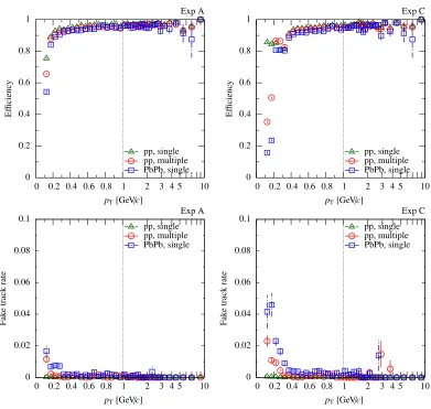
The proposed algorithm is coded in C++and run on a 2.1 GHz dual-core machine. The average CPU time needed was on average 25 sec for events with 40 simultaneous inelastic pp collisions. Its performance as a function of transverse momentum pT of the charged particles is shown in Fig. 6.

(A reconstructed track is considered matched to a simulated one if all their hits correspond to each other, or if at most one of them is not in place.) Efficiency and fake track rate are plotted for two experimental setups. The values are separately given for single pp, for multiple (40) simultaneous pp, and for semi-central PbPb collisions. It is clear that forpT >0.2–0.4 GeV/cthe efficiency is above

90–95% and fake track rate is well below 1%, independent of collision system (pp, PbPb) and pileup (1–40). At very low transverse momentum (pT <0.1–0.2 GeV/c) efficiency drops and fake track rate

increases to some 2–4%. Both measures show a clear advantage and convincing performance of the proposed methods over those presently used in the highest energy particle physics experiments.

0 0.2 0.4 0.6 0.8 1

0 0.2 0.4 0.6 0.8 1

E

ffi

cienc

y

pT[GeV/c]

2 3 4 5 10

Exp A

pp, single pp, multiple PbPb, single

0 0.2 0.4 0.6 0.8 1

0 0.2 0.4 0.6 0.8 1

E

ffi

cienc

y

pT[GeV/c]

2 3 4 5 10

Exp C

pp, single pp, multiple PbPb, single

0 0.02 0.04 0.06 0.08 0.1

0 0.2 0.4 0.6 0.8 1

F

ak

e

track

rate

pT[GeV/c]

2 3 4 5 10

Exp A

pp, single pp, multiple PbPb, single

0 0.02 0.04 0.06 0.08 0.1

0 0.2 0.4 0.6 0.8 1

F

ak

e

track

rate

pT[GeV/c]

2 3 4 5 10

Exp C

pp, single pp, multiple PbPb, single

Figure 6. Performance of the proposed algorithm as a function of transverse momentum pT of the changed

particles. Efficiency (top) and fake track rate (bottom) are plotted for Exp A (left) and Exp C (right). The values are separately given for single pp (open green triangles), multiple (40) pp (open red circles), and semi-central PbPb (open blue boxes) collisions. The horizontal scale is linear in the region 0–1 GeV/c, while it is logarithmic for 1–10 GeV/c.

decreases but stays in the 80–90% range. The fake track rate starts at the permille level and stays under a percent.

6 Summary

ro-0

0.2

0.4

0.6

0.8

1

0

10

20

30

40

50

60

70

80

E

ffi

cienc

y

Running

time

[s]

pp, multiple

10

10

0

10

20

30

40

50

60

70

F

ak

e

rate

Number of collisions

E

ffi

ciency

Running time

Fake rate

Figure 7. Performance of the proposed algorithm as a function of the number of simultaneous inelastic pp

collisions. Efficiency (open red circles, top left), running times (open blue diamonds, top right), and fake track rate (open green triangles, bottom) values are plotted. Lines are drawn to guide the eye.

tational symmetries of the detectors. Track candidates and their corresponding hits usually form a highly connected network, a graph. The graph is partitioned into very many minigraphs by removing a few of its vulnerable components, edges and nodes. The hits of a subgraph are distributed among the track candidates by solving a deterministic decision tree.

Tests using simplified computer models of LHC silicon trackers show that efficiency and purity of track reconstruction are excellent and the timing of the proposed method is reasonable, both in simultaneous proton-proton collisions (high pileup), and in single heavy-ion collisions at the highest available energies.

Acknowledgements

The author wishes to thank to Sándor Hegyi and András László for helpful discussions. This work was supported by the Swiss National Science Foundation (SCOPES 152601), and the National Research, Development and Innovation Office of Hungary (K 109703).

References

[1] G. Aad et al. (ATLAS), Eur. Phys. J. C76, 581 (2016),1510.03823 [2] M. Rovere (CMS), J. Phys. Conf. Ser.664, 072040 (2015)

[4] K. Aamodt et al. (ALICE), JINST3, S08002 (2008) [5] C. Cheshkov, Nucl. Instrum. Meth. A566, 35 (2006) [6] G. Aad et al. (ATLAS), JINST3, S08003 (2008)

[7] B. Mindur (ATLAS), Nucl. Instrum. Meth. A845, 257 (2017) [8] A. Strandlie, Nucl. Instrum. Meth. A535, 57 (2004)

[9] S. Chatrchyan et al. (CMS), JINST3, S08004 (2008)

[10] M. Lamont, Journal of Physics: Conference Series455, 012001 (2013) [11] C. Patrignani et al. (Particle Data Group), Chin. Phys. C40, 100001 (2016) [12] H. Bichsel, Rev. Mod. Phys.60, 663 (1988)

[13] R. Fruhwirth, Nucl. Instrum. Meth. A262, 444 (1987) [14] P.V.C. Hough, Tech. rep. (1962), US Patent 3069654

[15] T. Sjöstrand, S. Mrenna, P.Z. Skands, Comput. Phys. Commun.178, 852 (2008),0710.3820 [16] V. Khachatryan et al. (CMS), Phys. Lett. B751, 143 (2015),1507.05915

[17] J. Adam et al. (ALICE), Phys. Lett. B753, 319 (2016),1509.08734 [18] G. Aad et al. (ATLAS), Phys. Lett. B758, 67 (2016),1602.01633