Performance-based credit trading

PERFORMANCE-BASED CREDIT TRADING

by

Roger Salmons

PERFORMANCE-BASED CREDIT TRADING

by

Roger Salmons

Centre for Social and Economic Research on the Global Environment

University College London and

University of East Anglia

Acknowledgements

The Centre for Social and Economic Research on the Global Environment (CSERGE) is a designated research centre of the UK Economic and Social Research Council (ESRC).

Professor David Pearce, Dr. Malcolm Pemberton and Dr. Joe Swierzbinski of University College London provided valuable comments and suggestions on earlier drafts of this paper. However, any errors remain the responsibility of the author.

Abstract

It is well established that - in the absence of market distortions - permit trading provides a cost efficient implementation mechanism for a range of different environmental policy issues where objectives can be set - either explicitly, or implicitly - in absolute terms (e.g. tonnes of carbon). However in many policy areas, objectives are formulated in relative terms (i.e. as rates). For example, objectives may be set for energy efficiency rates in certain industrial sectors (i.e. energy consumption per unit output), or for the mix of secondary and primary materials used in the manufacture of certain products. Furthermore, in a second-best setting with distortionary taxes, there may be significant social cost advantages to using rate-based instruments, even when the underlying policy objective is expressed in absolute terms.

1. Introduction

It is well established that - in the absence of market distortions1 - permit trading provides a cost efficient implementation mechanism for a range of different environmental policy objectives. In particular, Montgomery (1972) shows that - where there is a linear relationship between (N) emissions sources and (M) pollution receptors - a system of tradable pollution licences (allowances) will ensure that environmental quality standards at each receptor point are met at least total cost. This general framework applies to a wide range of environ-mental policy concerns (e.g. acid rain, global warming, biological oxygen demand in water) where an absolute objective can be set - either explicitly as a quantity (e.g. X tonnes of carbon), or implicitly as a change versus a base year value (e.g. a X% reduction in greenhouse gas emissions from 1990 levels by 2010).

However in many policy contexts, especially at the national level, objectives are formulated in terms of relative objectives (i.e. as rates). For example, objectives may be set for energy efficiency rates in particular industrial sectors (i.e. energy consumption per unit of output); or for the mix of secondary (i.e. recycled) and primary material used in the production of certain products. Furthermore, even in a situation where the underlying policy objective is defined in absolute terms (e.g. an aggregate emissions limit for NOX for a

particular sector), there may be advantages in converting this to a “rate-based” regulatory rule, based on the expected level of activity (e.g. emissions of NOX

per unit of output). In a comparison of the cost efficiency of alternative policy instruments, Goulder et al., (1998) find that in a second-best setting with pre-existing factor taxes, the use of a performance standard to achieve a given absolute target can be significantly less costly to society than using an allocated (e.g. “grandparented”) permit scheme.2 While their analysis was primarily concerned with the tax interaction and revenue recycling impacts of the different instruments and did not consider the issue of implementation

1

Atkinson and Tietenberg (1991) discuss the issue of market failure in relation to emissions trading schemes; Hahn (1984) addresses the issue of market power; while Stavins (1995) considers the implications of transactions costs.

2

Goulder et al., (1998) undertake a numerical simulation of various different policy instruments for reducing NOX emissions in the USA. They find that, in the absence of

efficiency, it suggests that rate-based regulation may be an attractive policy option in many situations.3

However, in the same way that setting a common emissions limit for all firms is unlikely to be cost efficient, there is no reason to suppose that the imposition of a common performance rate will achieve the overall objective at least cost. Therefore, it would be of great benefit if some form of market mechanism could be found that would ensure the efficient implementation of this type of policy rule. To that end, this paper extends the analysis of the cost efficiency of trading schemes to encompass a broader range of regulatory rules, including those based on performance rates. It is demonstrated that a generic form of trading - “performance-based credit trading” - will achieve the cost efficient outcome for any policy objective that can be expressed in the form of a linear “performance rule”.

Definition 1

An aggregate performance rule for a group of firms (or sector4) is characterised by the constraint

α α α

α ⋅ ( _i

i y

=

å

1 N

) + K ≥ 0

where yi∈RM is the input-output vector for firm i, αααα∈RM is a vector of parameters, and K is a scalar constant.

This formulation is very flexible, and by choosing appropriate values for the vector α and the scalar K, it is possible to represent a variety of different regulatory rules, with a wide range of potential policy applications. To illustrate this, let the input-output vector be partitioned into (yi | wi | zi) where

yi∈RJ is a vector of outputs, wi∈RK- is a vector of market inputs (e.g. different types of energy), zi∈RL- is a vector of non-market inputs (e.g. emissions of air

3

The analysis assumed that firms were homogeneous, and that initial allocations of permits were identical. Therefore the initial distribution of permits was cost efficient, and the issue of trading did not arise.

4

pollutants5); and partition the parameter vector correspondingly into (αααα | ββββ | γγγγ). As can be seen in Table 1, by choosing appropriate values for the vectors αααα, ββββ and γγγγ and the scalar Kit is possible to generate a number of different types of regulatory rule. In particular, the general formulation can incorporate relative (or “rate based”) targets such as those illustrated by the last two cases - i.e. energy efficiency and minimum recycled content.

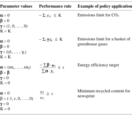
Table 1: Examples of linear performance rules

Parameter values Performance rule Example of policy application

αααα = 0

ββββ = 0

γγγγ = (1, 0, … , 0) K = K

− Σi z1i ≤ K Emissions limit for CO2

αααα = 0

ββββ = 0

γγγγ = (γ1, … , γL)

K = K

− Σiγγγγ⋅zi ≤ K Emissions limit for a basket of

greenhouse gases

αααα = (rα1, … , rαJ)

ββββ = ββββ

γγγγ = 0 K = 0

−_å ⋅ ⋅ å ≤ ββββ αααα i i w y i i

r Energy efficiency target

αααα = 0

β = (-1, r, 0, … , 0)

γγγγ = 0 K = 0

1 2 w w ≥

r Minimum recycled content for

newsprint

In the next section, the cost efficient outcome under the generalised performance rule is characterised, and its existence is proved. Section 3 then outlines the mechanics of performance-based credit trading (PBCT), and the necessary and sufficient conditions are derived for a market equilibrium in

5

2. Cost Efficient Regulation

For the purposes of the analysis, it is assumed that the regulatory rule applies to a specific sector of the economy, which comprises a fixed number of firms (N). The production set of firm i∈I6 is denoted by:

Gi = { (yi| wi | zi) ; gi(yi | wi | zi) ≤ 0 }

where yi∈RJ is a vector of outputs; wi∈RK- is a vector of market inputs; and

zi∈RL- is a vector of non-market inputs. It is assumed that for all i∈I, Gi is closed with a non-empty interior, and that the transformation function

gi(yi | wi | zi) is continuous and strictly convex.

The vector (y | w | z) denotes the overall production plan for the sector, where

y = (y1 | … | yN), w = (w1 | … | wN) and z = (z1 | … | zN). The sector production

set is denoted by:

G = { (y| w | z) ; (yi| wi | zi) ∈ Gi ∀ i∈I }

It follows directly that the set G is also closed with a non-empty interior.

For a specified aggregate performance rule (PR), the set of “allowable” sector production plans is given by the closed half-space:

S = { (y| w | z) ; αααα~⋅y+ ββββ~⋅w + ~γγγγ⋅z + K ≥ 0 } 7

Given the general formulation of the performance rule, it is possible that for certain parameter values there may be no technically feasible production plan (y | w | z) which also satisfies the rule. In order to avoid this possibility, the notion of a technically feasible performance rule is introduced.

6

The set I is the set of integers {1, 2, …, N}. Similar notation is used for the sets J and K.

7 _αααα~

is the (×N) repeated vector of parameters (αααα | … | αααα). Hence αααα ⋅~ y = αααα⋅(Σi yi). Similarly

Definition 2

A performance rule is technically feasible if there exists (yi | wi | zi) ≠ 0

∀ i∈I , such that:

a) gi(yi | wi | zi) < 0 ∀ i∈I ; and

b) αααα~⋅y + ~ββββ⋅w + ~γγγγ⋅z + K > 0 i.e. if the set G ∩ S has a non-empty interior.

It is assumed that in the absence of any regulatory rule, there exists a finite solution to each firm’s “unregulated” optimization problem (UPi)

8

, and that the resultant profit of each firm i∈I is given by πiu = py⋅yiu + pw⋅wiu; where py > 0 is a J-dimension vector of exogenous output prices; and pw > 0 is a K-dimension vector of exogenous input prices.9 Consequently, the maximized aggregate profit for the sector is given by Πu = p~y⋅yu + p~w⋅wu.10

The cost associated with a particular sector production plan (y | w | z) ∈ G ∩ S is defined to be Πu - (~py⋅y + p~w⋅w) . A production plan (y*| w*| z*) is cost efficient if it minimizes this difference. Since the reference level of profit (Πu) is unaffected by the choice of production plan, this is equivalent to finding the plan which maximizes sector profit under the performance rule.

More formally, a production plan (y*| w*| z*) is cost efficient if it is a solution to the following problem (CE):

8

Maximize py⋅yi + pw⋅wi subject to gi(yi | wi | zi) ≤ 0

yi wi zi

9

The assumption of exogenous prices has been made to allow the analysis to focus solely on the market in performance credits. It reflects a situation where the sector is not sufficiently large to affect input prices, and sells its output in international markets. The use of alternative assumptions to close the model (e.g. downward sloping demand curves, etc) would not affect the conclusions of the analysis.

10 y

p

~ _{is the (×N) repeated vector of parameters (p}y

| … | py). Hence ~py⋅yu = py ⋅(Σi yiu).

Maximize p~y⋅ y + p~w⋅ w y, w, z

subject to (y| w | z) ∈ G ∩ S

Given the convexity of the transformation functions and the performance rule, if the performance rule is technically feasible (see Definition 2), then the Slater constraint qualification is satisfied.11 Therefore, if (y*| w*| z*) is a solution to CE, then there exist non-negative multipliers µi* ∀ i∈I and η∗, such that yji

*

, wki*, zli*, µi* and η*satisfy the following first-order conditions for all i∈I:

pyj - µi g i

j + η αj = 0 ∀ j∈J,

pwk - µi g i

k + ηβk≤ 0 wki [pwk - µi g i

k + ηβk] = 0 ∀ k∈K

- µigil + η γl ≤ 0 zli [- µig i

l + ηγl ] = 0 ∀ l∈L

gi(yi, wi, zi) ≤ 0 µi [ g i

(yi, wi, zi) ] = 0

and

~

αααα⋅y + ββββ~⋅w + ~γγγγ⋅z + K ≥ 0 η [αααα~⋅y + ~ββββ⋅w + ~γγγγ ⋅z + K] = 0

Since the objective function is linear, and each constraint function is convex, these conditions are also sufficient. Hence, if there exists a vector (y*| w*| z*) satisfying the above set of first-order conditions, it is a global maximizer of the cost efficiency problem (CE).

Proposition 1

If there exists a finite solution to each firm’s “unregulated” optimization problem (UPi); and if the performance rule is technically feasible; then

there exists a finite solution to the cost efficiency problem (CE).

Proof : see appendix 1

11

Interpretation of the first-order conditions is facilitated by the assumption of a “non-corner” solution (y*| w*| z*), in which case the following I×(J×(K+L)+1)+1 conditions characterize completely the cost efficient solution:

pwk + η

*_βk

= (gik

*

/ gij

*

) ( pyj + η

*_αj

) ∀ i∈I, k∈K, j∈J (CE1)

η*_γl

= (gil

*

/ gij

*

) ( pyj + η

*_αj

) ∀ i∈I, l∈L, j∈J (CE2)

gi(yi

*

, wi

*

, zi

*

) = 0 ∀ i∈I (CE3)

~

αααα⋅y* + ~ββββ⋅w* + ~γγγγ ⋅z* + K = 0 (CE4)

The marginal product conditions (CE1) and (CE2) show how the market prices must be amended in order to induce a cost efficient solution. Depending on the exact nature of the performance rule (i.e. the specific values of the elements of the parameter vector (αααα | ββββ | γγγγ)), adjustments may be required to input prices, or to output prices, or to both.12 For an aggregate emissions limit (i.e. Table 1 -cases 1), the prices of all marketed inputs and outputs remain unaltered (i.e. αααα =

ββββ = 0); the only change being to the I×J conditions for the pollutant in question, where the value of the marginal product is now set equal to the shadow price of associated non-market input (η*). Similarly, if a constraint is imposed on the relative levels of two specific marketed inputs (i.e. Table 1 - case 4), then it is only the 2×I×J conditions relating to these inputs that are affected, with the input prices being increased by η* and r η* respectively.

12

3. Performance-Based Credit Trading

Under performance-based credit trading (PBCT), each firm i∈I is subject to an individual performance rule (PRi), of the form:

αααα⋅yi + ββββ⋅wi + γγγγ⋅zi + k + ai ≥ 0

The parameter vectors αααα, ββββ, and γγγγ are the same as those that apply to the aggregate rule (PR), and k = (1/N)×K. However, the individual rule includes an extra term (ai), which represents an individual “performance adjustment factor”

for each firm i∈I. This factor allows the distributional impacts of the aggregate performance rule to be varied. For example, if K represents an absolute aggregate target (e.g. case 1 in Table 1), then if ai > 0 the individual target for

firm i (i.e. k + ai) is above the average, and if ai < 0 it is below. In terms of

traditional “allowance” trading schemes, this is equivalent to varying the initial distribution of a fixed number of permits.

However, if the actual production plan (yi | wi | zi) of firm i∈I is such that this

satisfies the performance rule (PRi) as a strict inequality, then it is allowed to

generate “performance credits” which it can sell to other firms in the sector. The purchasing firm can use these credits towards satisfying its performance rule. However, net of all transactions, each firm must satisfy its own individual performance rule. Thus, if ci represents the number of credits bought or sold by

firm i∈I (ci < 0 for purchases and ci > 0 for sales), then the set of “allowable”

augmented production plans for firm i∈I is given by:

Si = { (yi| wi | zi | ci) : αααα⋅yi + ββββ⋅wi + γγγγ⋅zk+ k + ai - ci ≥ 0 }

Definition 3

Given exogenous price vectors py and pw, a competitive market equilibrium for performance credits comprises a scalar price qc** ≥ 0, and vectors y**, w**, z**, and c**, such that yi

**

, wi **

, zi **

, and ci **

a) solve each firms “regulated” optimization problem (RPi); i.e.

maximize py⋅yi + pw⋅wi + qc**ci

yiwizi ci

subject to (yi| wi | zi) ∈ Gi

(yi| wi | zi | ci) ∈ R i

for all i∈I;

b) satisfy the market clearing conditions (MC); i.e.

Σi ci ≥ 0 ; qc ( Σi ci ) = 0 ; qc≥ 0

For each firm i∈I, the constraint qualification is satisfied13. Therefore, if (yi

**

| wi **

| zi **

| ci

**

) is a solution of RPi, then there exist non-negative multipliers µi** ∀ i∈I and ηi** ∀ i∈I, such that yji**, wki**, zli**, ci**, µi** and ηi**satisfy the

following conditions ∀ i∈I:

pyj - µi g i

j + ηiαj = 0 ∀ j∈J

qc** - ηi = 0

pwk - µi g i

k + ηi βk ≤ 0 wki [pwk - µi g i

k + ηi βk] = 0 ∀ k∈K

- µigil + ηi γl ≤ 0 zli [- µigil + ηiαl ] = 0 ∀ l∈L

gi(yi | wi | zi) ≤ 0 µi [ gi(yi | wi | zi) ] = 0

αααα⋅yi + ββββ⋅wi + γγγγ⋅zi+ k + ai - ci ≥ 0 ηi [ αααα⋅yi + ββββ⋅wi + γγγγ⋅zi+ k + ai -ci ] = 0

13

Again, since the objective function is linear, and each constraint function is convex, these conditions are also sufficient and therefore, if there exists

(yi**| wi**| zi**| ci**) satisfying this set of first-order conditions, it is a global

maximizer of the firms “regulated” optimization problem (RPi). Consequently,

these conditions for each i∈I, together with the market clearing condition (MC) are necessary and sufficient for the existence of a market equilibrium.

Proposition 2

For any technically feasible aggregate performance rule, if Σi ai = 0,

then a market equilibrium for performance credits exists

Proof : see appendix 2

Furthermore:

Proposition 3

If Σi ai = 0, then any market equilibrium for performance credits is a

solution to the cost efficiency problem (CE)

Proof : see appendix 3.

Thus, provided that the individual adjustment factors are set such that they sum to zero (i.e. there is no net adjustment to the rule in aggregate), one can conclude that not only will a market equilibrium for performance credits be guaranteed to exist, but also the resultant outcome will achieve the overall performance target at least cost.14 The second part of this statement can be seen if one again assumes a “non-corner” solution, in which case the market equilibrium can be characterised completely by the following set of I×(J×(K+L)+2)+1 conditions:

14

pwk + q

c**_βk

= (gik

**

/ gij

**

) ( pyj + q

c**_αj

) ∀ i∈I, k∈K, j∈J (ME1)

qc**γl = (gil

**

/ gij

**

) ( pyj + q

c**_αj

) ∀ i∈I, l∈L, j∈J (ME2)

gi(yi

**

| wi

**

| zi

**

) = 0 ∀ i∈I (ME3)

αααα⋅yi **

+ ββββ⋅wi **

+ γγγγ⋅zi∗∗+ k + ai - ci

**

= 0 ∀ i∈I (ME4)

Σi ci

**

= 0 (ME5)

Taken together, conditions ME4 and ME5 imply that:

~

αααα⋅y + ~ββββ⋅w + ~γγγγ⋅z + K + Σi ai = 0 (ME4a)

Comparing ME1-ME4a with CE1-CE4, it is clear that if Σi ai = 0, then the two

4. Application of PBCT to Energy Efficiency

An interesting potential policy application of PBCT is in the area of industrial energy efficiency, where a target rate is set for aggregate energy consumption per unit of output for a particular sector. In this case the generic performance rule parameters take the values: αααα ≡ (rα1, … rαJ); ββββ ≡ (β1, … , βk, 0, … , 0)

15

;

γγγγ = 0; K = 0; where the scalar r is the target energy efficiency rate for the sector, and the vectors αααα and ββββk represent conversion factors for the different types of

output and energy inputs. The aggregate performance rule becomes:

r αααα⋅(Σiyi) + ββββ⋅(Σiwi) ≥ 0 or equivalently −å ⋅

⋅ å ≤ ββββ αααα i i w y i i r

The first term (or denominator) represents the total output for the sector in common units (e.g. tonnes), while the second term (or numerator) represents the total amount of energy consumed by the sector in common units (e.g. kJ). Assuming a “non-corner” solution, the cost efficient solution requires that the marginal product conditions for each firm satisfy:

pwk + η

*_βk

= - (gik

*

/ gij

*

) ( pyj + η

*_αj

) ∀ i∈I, j∈J, k = 1, …, k

pwk = - (g

i k

*

/ gij

*

) ( pyj + η

*_αj

) ∀ i∈I, j∈J, k = k+1, …, K

Thus, not only does cost minimisation under an energy efficiency constraint change the marginal product condition for each energy input (k = 1, …, k), it also changes the marginal product conditions for all other inputs. This reflects the fact that, due the inclusion of output in the performance rule, the shadow price of each output j is increased by an amount η*αj.

The “post-trading” performance rule for firm i is given by:

r αααα⋅yi + ββββ⋅wi + ai -ci ≥ 0 or equivalently

− ⋅ + ⋅ ≤ ⋅ ββββ αααα αααα i i i w y y i i

c _{r +} a

15

from which it can be seen that - in this case - the performance credits are denominated in units of energy.

If the adjustment factors are set to zero for each firm (i.e. ai = 0 ∀ i∈I) then,

after trading has taken place, each firm must achieve the same energy efficiency rate (r). However, by setting non-zero adjustment factors it is possible to vary the “effective” target efficiency rates between different firms (or groups of firms), i.e. if ai < 0 then the firm faces a more stringent efficiency target than

the sector average. It should be noted that while the adjustment factor (ai) is

constant, the impact of the factor on the target rate is not. The latter will vary depending on the level of the firm’s output - reducing in magnitude as output increases.

While PBCT will ensure that the aggregate cost of meeting the sector efficiency target is minimized irrespective of the individual values of ai (provided that Σi

ai = 0), the cost burden on individual firms will depend critically on these

values. For example, if “pre-regulation” energy efficiency rates vary significantly across the sector, a common target rate is likely to result in widely differing cost burdens on individual firms. However, if the divergence of performance reflects genuine differences in the characteristics of individual firms, such an outcome may be hard to justify. For example, the sector may comprise a number of distinct sub-sectors with substantially different inherent energy intensities.

The inclusion of the adjustment factors in PBCT provides a flexible mechanism that can be used to address this issue. In particular, it allows a number of different approaches to be adopted for the determination of the adjustment factors. If information is available, then values could be calculated on the basis of the expected costs of improved energy efficiency to individual firms (or sub-sectors). Alternatively a more mechanistic approach could be adopted, with adjustment factors calculated on the basis of a pre-determined rule.16 One such rule might be that each firm should be required to make the same percentage improvement in its energy efficiency rate.17 This rule can be considered as the

16

While the use of expected cost information would in theory allow the calculation of adjustment factors that reflected some notion of fairness (e.g. ability to pay), in practice a mechanistic rule may prove to be more acceptable to the constituent firms.

17

performance-based equivalent of the use of grandparenting as the allocation rule for “allowance” permits.

Suppose that prior to the introduction of any regulation, the actual energy efficiency of each firm is ~r and that the overall energy efficiency of the sectori is ~r, where:

i

~ ~

~

r = − ⋅

⋅ ββββ αααα i i w y and ~ ~ ~

r = − ⋅

⋅

å

å

If the aggregate target rate for the sector is r then, under this rule, the target performance rate for firm i would be

( )

(

)

(

)

i

a r

r ri r

= æ_èç~ö_ø÷ ~ −~ _αααα⋅~

i y

The sign of the adjustment factor for a particular firm depends on whether its (pre-regulation) performance rate is above or below the sector average; while the relative magnitude of the factor depends on the extent to which its rate differs from the average, and on its actual energy consumption. It is straightforward to show that the adjustment factors calculated under this rule satisfy the requirement that Σi ai = 0.

Σi ai =

(

)

(

)

r

r ri r

~ ~ ~ ~

æ

èç öø÷

å

= −æ

[

]

èç öø÷

å

å

r r~

~ ~

ββββ wi ββββ wi

i i = 0

When this adjustment factor is applied, the performance rule for firm i becomes:

− ⋅ +

⋅ ≤ + æèç − öø÷

⋅ ⋅

é ë

ê ù

û ú

ββββ αααα

αααα αααα i

i

i i

i w

y i

c _r r

r

1 ~_~ 1

~_y

y

5. Discussion

The preceding analysis has shown that it is possible to use a generic trading mechanism - performance-based credit trading (PBCT) - to achieve the cost efficient implementation of any regulatory objective that can be expressed in the form of a linear performance rule. Furthermore, the use of performance adjustment factors allows the distributional impact of the rule to be varied, to reflect either normative concerns of equity and fairness, or pragmatic concerns of political acceptability.

It is important to note that cost efficiency is defined relative to the specified performance rule, which need not necessarily be the same as the underlying policy objective. For example, the former may be expressed in terms of a rate (e.g. tonnes of carbon per unit of output) while the latter is defined in terms of an absolute quantity (e.g. tonnes of carbon). In this case, if there are no distortionary taxes in the economy, then PBCT will not lead to the cost efficient achievement of the policy objective as it does not induce the necessary reduction in output. However as was noted in section 1, in the presence of distortionary taxes, an efficiently implemented rate-based performance rule may often be less costly than a quantity-based instrument.

While PBCT is of particular relevance for the implementation of rate-based performance rules, it can also be used in the case of an absolute (or quantity-based) performance rule such as an aggregate limit on the emissions of a particular pollutant. For a regulatory rule of this type, the individual performance rule for a firm i is given by:

- zk + ci ≤ ki (where ki = k + ai ; and Σi ki = K)

which is exactly the same as the rule that the firm would face under an “allowance” permit trading scheme when it receives an initial allocation of permits equal to ki.

However, while PBCT and permit trading are functionally equivalent, they differ fundamentally in terms of property rights. Under permit trading, the firm is given property rights in relation to its entire initial allocation (i.e. ki) and it is

free to transfer any proportion of these rights to another party. In contrast, under PBCT, the firm can only generate property rights up to the amount by which it beats its individual target (i.e. ki - (- zk)). This distinction could have

trading, particularly if past permit allocations are considered by firms to confer de facto future property rights.

The analysis of PBCT undertaken here assumes that there is a fixed number of firms in the sector, and hence no consideration has been given to the issue of entry and exit. In the special case of an undifferentiated rate-based rule (for example, where all firms in the sector face a common energy efficiency target), it is clear that the entry and exit of firms will not affect the cost efficient achievement of the aggregate target. In all other cases, some provision must be made to deal with this issue. One possible approach that could be adopted in the case of a differentiated rate-based rule, would be set the value of the adjustment factors such that Σi ai < 0, with the balance being held by the

References

Atkinson, S. and Tietenberg, T.H. (1991). “Market failure in incentive-based regulation: The case of emissions trading”, Journal of Environmental Economics and Management, Vol 21, pp 17-31

Goulder, L.H., Parry, I.W.H., Williams III, R.C. and Burtraw, D. (1998). “The Cost-Effectiveness of Alternative Instruments for Environmental Protection in a Second-Best Setting”, Discussion Paper 98-22, Resources for the Future, Washington DC, USA.

Hahn, R.W. (1984). “Market power and transferable property rights”, Quarterly Journal of Economics, 100, pp 753-765

Montgomery, W.D. (1972). “Markets in licences and efficient pollution control programs”, Journal of Economic Theory, 5, pp 395-418

Simon, C.P. and Blume, L (1994). Mathematics for Economists, New York, Norton

Appendix 1 : Proposition 1

If: (i) for each firm i∈I there exists a solution (yi*) to the “unregulated” problem, max

p⋅ yi s.t. yi ∈ Gi , where Gi = { yi ∈ RM; gi(yi) ≤ 0} is closed, and the

transformation function gi(yi) is continuous and strictly convex;

(ii) the performance rule is technically feasible, i.e. the set G ∩ S has a non-empty interior, where G = { y∈ RNM; yi∈ Gi∀ i∈I } and

S = { y∈ RNM; ~αααα ⋅y ≥ - K };

then there exists a solution to the aggregate “regulated” problem, max ~p⋅y s.t. y∈ G ∩ S, where y = (y1 | … | yN) and ~p = (p | … | p).18

Proof:

• Since by assumption there exists a solution to each firms unregulated problem, it follows directly that there exists a solution19 (Π* = ~p⋅ y* = p~⋅ (y1* | ………… | yN*)) to the aggregate

“unregulated” problem, max ~p⋅y s.t. y ∈ G. Consequently, the supporting hyperplane for G at y* is given by ~p⋅y = Π*.

• Take any vector y/ ∈ Int (G ∩ S), with ~p⋅ y/ = Π/ < Π*, and let A/ = { y ; ~p⋅y ≥Π/ }. By Lemma 1 (see below), the set G ∩ A/ is compact.

• Since the half-space S is closed, it follows that B = S ∩ (G ∩ A/) is closed, and hence that B ⊂ (G ∩ A/) is compact.

• Therefore, since the profit function ~p⋅ y is continuous, by Weierstrass’s Theorem, there exists a solution (y**) to the problem, max ~p⋅y s.t. y ∈ B = (G ∩ S) ∩ A/.

• However, by construction there exists some vector y//∈ G ∩ S , with ~p⋅ y// > Π/, which implies that ~p⋅ y** > Π/. Hence, the constraint associated with the set A/ is not binding, and its removal will not change the solution. Therefore, the vector y** is also a solution to the problem, max ~p⋅y s.t. y ∈ G ∩ S.

Q.E.D.

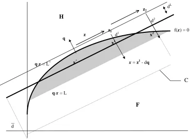
Lemma 1

If : (i) for all i∈I, Fi = { xi ∈ RK ; fi(xi) ≤ 0} is closed, with fi(xi) continuous and

strictly convex;

(ii) q ⋅x = L* is the supporting hyperplane for F at the point x* (x*∉ Int F), where

x = (x1 | … | xN) and F = { x ; xi∈ Fi∀ i∈I };

(iii) H = { x ; q ⋅x ≥ L};

then for any L ≤ L*, the set F ∩ H is compact (i.e. closed and bounded).

Figure A1 : Example with N=1 and K=2

Proof:

F ∩ H is closed

• The half-space H is closed by definition, and each set Fi is closed by assumption. Therefore, it follows directly that F is closed, and hence that F ∩ H is also closed. F ∩ H is bounded

• Note that the distance between the supporting hyperplane q ⋅ x = L* and an arbitrary “parallel” hyperplane q ⋅ x = L ≤ L* (i.e. the distance along the line orthogonal to the two hyperplanes), is given by dL = (L* - L) / || q ||.

dL

z2

d2

x2

d1

x1 z1

z q

x*

f(x) = 0

q⋅x= L*

q⋅x= L H

F

d

x = z1 - dq

• Consider a vector z, with || z || = 1, in any arbitrary direction such that q ⋅ z = 0, and construct a sequence of points {zm}m = 0…∞ along the surface of the supporting hyperplane

q ⋅x = L*, where zm = x* + mz, and hence || x* - zm || = m.

• For each point zm, construct the normal line x = zm - dq (where d is some scalar), and let xm = argminx { || zm - x || ; x = zm - dq for some value of d, and fi(xi) ≤ 0 for all i∈I }, with

dm = || zm - xm || (see Figure A1 for example with N=1 and K=2).

Note that since fi(xi) is continuous and strictly convex for all i∈I, it must be the case that

for all m, fi(xim) = 0 for some i∈I and dm > 0.

• Since fi(xi) is strictly convex for all i∈I, it must be the case that dm+1 - dm > dm - dm-1. If

this is not so then, by construction, the line joining xm-1 and xm+1 will intersect the normal line x = zm - dq at the point xm= 0.5 xm-1 + 0.5 xm+1, with || zm - xm|| ≤ || zm - xm ||. But since each fi(xi) is strictly convex, it follows directly that fi(xim) < 0 for all i∈I. Therefore,

since each fi(xi) is continuous, there exists a vector xm such that fi(xim) < 0 for all i∈I and

|| zm - xm|| < || zm - xm|| ≤ || zm - xm ||, which contradicts xm being the argmin.

• Therefore, {dm}m = 0…∞ is a divergent, monotonically increasing sequence. Hence for any

value of dL, and an arbitrary direction vector z along the supporting hyperplane, there exists a finite value M such that for all m < M, dm≤ dL, and for all m ≥ M, dm > dL.

• Therefore, it is possible to construct an (N×K)-dimensional “cylinder” C around an axis defined by the line x = x* - dq, with finite radius M and length d (where M is the maximum value of M, and d is the maximum value of dM, across all possible direction vectors z), such that for all x∉ C, either q ⋅x < L, or fi(xi) > 0 for some i∈I, or both (see

Figure A1). Hence (F ∩ H) ∩ Cc = ∅, which implies that F ∩ H is bounded.

Appendix 2 : Proposition 2

For any technically feasible performance rule, if Σi ai = 0, then a market equilibrium for performance credits exists.

Proof:

By Proposition 1, for any technically feasible performance rule, there exist vectors y**≥ 0, w*≤ 0, z*≤ 0, and µµµµ*≥ 0, and a scalar η∗*≥ 0, such that the necessary and sufficient conditions for a cost efficient solution are satisfied, i.e. (∀ i∈I):

pyj - µi* gij* + η∗αj = 0 ∀ j∈J

pwk - µi*gik* + η∗βk≤ 0 wki*[ pwk - µi*gik* + η∗βk ] = 0 ∀ k∈K - µi*gil* + η∗γl ≤ 0 zli*[- µi*gil* + η∗γl] = 0 ∀ l∈L gi(yi*| wi*| zi*) ≤ 0 µi*[ gi(yi*| wi*| zi*) ] = 0

and

~

αααα ⋅y* + ββββ ⋅~ w* + ~γγγγ ⋅z* + K ≥ 0 η* [αααα ⋅~ y* + ~ββββ ⋅w* + ~γγγγ ⋅z* + K] = 0

Now consider the final complementary slackness condition (relating to the performance rule). If Σi ai = 0, then this condition can be restated (in expanded form) as:

Σi [αααα⋅yi* + ββββ⋅wi* + γγγγ⋅zi* + K + ai] ≥ 0 η∗[Σi [αααα⋅yi* + ββββ⋅wi* + γγγγ⋅zi* + K + ai] = 0

(i) If η∗ > 0, then Σi [αααα⋅yi* + ββββ⋅wi* + γγγγ⋅zi* + K + ai] = 0.

Therefore, there exists c* = (c1*, … , ci*, … , cN*) with Σi ci* = 0 , such that

αααα⋅yi* + ββββ⋅wi* + γγγγ⋅zi* + k + ai - ci* = 0 ∀ i∈I. (NB: k = K/N)

(ii) If η∗ = 0, then Σi [αααα⋅yi* + ββββ⋅wi* + γγγγ⋅zi* + K + ai] ≥ 0.

Therefore, there exists d* = (d1*, … , di*, … , dN*) with Σi di*≥ 0 , such that

Σi [αααα⋅yi* + ββββ⋅wi* + γγγγ⋅zi* + K + ai - di*] = 0

Therefore, there exists δδδδ* = (δ1*, … , δi*, … , δN*) with Σiδi* = 0 , such that

αααα⋅yi* + ββββ⋅wi* + γγγγ⋅zi* + k + ai - di* - δi* = 0 ∀ i∈I

Thus the final complementary slackness condition implies that for any cost minimum solution there exists some vector c* such that the following I+1 conditions are satisfied for all i∈I:

αααα⋅yi* + ββββ⋅wi* + γγγγ⋅zi* + k + ai -ci* = 0 η∗[ αααα⋅yi* + ββββ⋅wi* + γγγγ⋅zi* + k + ai -ci*] = 0

Σi ci*≥ 0 η∗[Σi ci*] = 0

Now let:

yi** = yi* ; wi** = wi* ; zi** = zi* ; µµµµi** = µµµµi* ∀ i∈I

ci** = ci* ; ηi** = η* ∀ i∈I

qc** = η*

then it follows directly from the above that ∀ i∈I:

pyj - µi** gij** + η∗∗αj = 0 ∀ j∈J

- qc** + ηi** = 0

pwk - µi**gik** + η∗∗βk≤ 0 wki**[ pwk - µi**gik** + η∗∗βk ] = 0 ∀ k∈K - µi**gil** + η∗∗γl ≤ 0 zli**[- µi**gil** + η∗∗γl] = 0 ∀ l∈L gi(yi**| wi**| zi**) ≤ 0 µi**[ gi(yi**| wi**| zi**) ] = 0

αααα⋅yi** + ββββ⋅wi** + γγγγ⋅zi** + k + ai - ci** = 0

ηi∗∗[ αααα⋅yi** + ββββ⋅wi** + γγγγ⋅zi** + k + ai -ci**] = 0

and

Σi ci**≥ 0 qc∗∗[ Σi ci** ] = 0 qc∗∗≥ 0

Thus, the necessary and sufficient conditions for a market equilibrium for performance credits are satisfied.

Appendix 3 : Proposition 3

If Σi ai = 0, then any market equilibrium for performance credits is a solution to the cost efficiency problem (CE).

Proof:

From the necessary and sufficient conditions for a market equilibrium for performance credits, comprising a scalar price qc** ≥ 0: and vectors y**≥ 0, w**≤ 0, z**≤ 0 and c**, there exist vectors of multipliers µµµµ**≥ 0 and ηηηη**≥ 0 such that following conditions are satisfied ∀ i∈I:

pyj - µi** gij** + ηi∗∗αj = 0 ∀ j∈J

- qc** + ηi** = 0

pwk - µi**gik** + η∗∗βk≤ 0 wki**[ pwk - µi**gik** + η∗∗βk ] = 0 ∀ k∈K - µi**gil** + η∗∗γl ≤ 0 zli**[- µi**gil** + η∗∗γl] = 0 ∀ l∈L gi(yi**| wi**| zi**) ≤ 0 µi**[ gi(yi**| wi**| zi**) ] = 0

αααα⋅yi** + ββββ⋅wi** + γγγγ⋅zi** + k + ai -ci** ≥ 0

ηi∗∗[ αααα⋅yi** + ββββ⋅wi** + γγγγ⋅zi** + k + ai -ci**] = 0 ∀ i∈I

and

Σi ci**≥ 0 qc∗∗[ Σi ci** ] = 0

The last two complementary slackness conditions, together with the condition that qc** = ηi**

∀ i∈I, imply that:

Σi[αααα⋅yi** + ββββ⋅wi** + γγγγ⋅zi** + ai ] + K ≥ 0

qc**[Σi[αααα⋅yi** + ββββ⋅wi** + γγγγ⋅zi** + ai ] + K] = 0 qc**≥ 0

Now let:

yi* = yi** ; wi* = wi** ; zi* = zi** ; µi* = µi** ; ∀ i∈I

η*

= qc**

pyj - µi* gij* + η∗αj = 0 ∀ j∈J pwk - µi*gik** + η∗βk≤ 0 wki*[ pwk - µi*gik* + η∗βk ] = 0 ∀ k∈K - µi*gil* + η∗γl ≤ 0 zli*[- µi*gil* + η∗γl] = 0 ∀ l∈L gi(yi*| wi*| zi*) ≤ 0 µi*[ gi(yi*| wi*| zi*) ] = 0

and

~

αααα ⋅y* + ββββ ⋅~ w* + ~γγγγ ⋅z* + K ≥ 0 η* [αααα ⋅~ y* + ~ββββ ⋅w* + ~γγγγ ⋅z* + K] = 0

Thus, the necessary and sufficient conditions for a cost minimum are satisfied.