Numerical precision of the solution to the running-coupling Balitsky-Kovchegov equation

(1)

Numerical precision of the solution to the running-coupling

Balitsky-Kovchegov equation

Marek Matas1,a, Jan Cepila1_{, and Jesus Guillermo Contreras Nuno}1

1_{Faculty of Nuclear Sciences and Physical Engineering, Czech Technical University in Prague, Prague,}

Czech Republic

Abstract.We use the running coupling Balitsky-Kovchegov (rcBK) equation to study the rapidity dependence of saturation in inclusive HERA data and we discuss the behaviour of its numerical solution. The rcBK equation has been solved using Runge-Kutta meth-ods. The inﬂuence of the parameters implicit in the numerical evolution has been studied. They include, among others, the order of the Runge-Kutta evolution, the size of the dif-ferent grids and the step in the numerical evolution. Some suggestions on the minimum value of these parameters are put forward.

1 Introduction

One of the open questions in particle physics is particle production in the high-energy limit of QCD. Evolution equations such as BFKL [1–5] are used to describe the gluon density of the hadron in high-energy collisions. The BFKL evolution equation predicts the emergence of new partons as the high-energy of the collision increases and in this approach, the gluon density is not bound by unitarity restrictions. The number of partons may be reduced by saturation eﬀects caused by recombination processes inside the hadron. An extension of the BFKL equation was found by Balitsky [6] and Kovchegov [7] (BK) resulting in an equation that generates dynamical balance between radiation and recombination pro-cesses driven by a saturation scale. The integro-diﬀerential BK evolution equation [8–10] considered in this work, and denoted by rcBK in the following, includes a running-coupling kernel that takes into account two-loop processes and assumes an impact-parameter independent solution [11]. It was derived from the JIMWLK evolution equations in the limit of large number of colors by Kovchegov [7, 12].

Using numerical methods one can solve the rcBK equation [8–10, 13] and calculate a prediction for the proton structure of DIS that accounts for recombination processes within the hadron. Numer-ical methods used to compute the rcBK solution need to be studied and an optimal setup regarding precision and speed of computation has to be tested in order to estimate the uncertainty coming from the non-analytic solution of rcBK equation.

2 The rcBK evolution equation

The rcBK evolution equation with running coupling kernel reads [14].

(2)

∂N(r,Y)

∂_Y =

dr1Krun(r, r1, r2)(N(r1,Y)+N(r2,Y)−N(r,Y)−N(r1,Y)N(r2,Y)), (1)

whereKrun₍_r_,_r

1, r2) can be expressed as [15]

Krun(r, r1, r2)= Nc

α_s(r2₎

2π2

⎛ ⎜⎜⎜⎜⎝ r2

r2 1r 2 2 + 1 r2 1 ⎛ ⎜⎜⎜⎜⎝α_s(r2

1)

α_s(r2 2)

−1

⎞ ⎟⎟⎟⎟⎠+ 1

r2 2

⎛ ⎜⎜⎜⎜⎝α_s(r2

2)

α_s(r2 1)

−1

⎞

⎟⎟⎟⎟⎠⎞⎟⎟⎟⎟⎠, (2)

r2 =r−r1andY =lnx_x0 . If we disregard the last term in Eq.1, we obtain a linear equation that

can be shown to be equivalent to the BFKL evolution equation [16]. The running coupling depends on the number of considered quark ﬂavors, in this work we usenf =3

α_s,nf(r

2₎₌ 4π

β0,nfln 4C2

r2_Λ2 n f

, (3)

where

β0,nf =11−

2

3nf. (4)

The constantC2 _{is the uncertainty coming from the Fourier transformation and is usually ﬁtted}

to data [10],Λ2

nf is called the scale parameter and its value depends on the value ofnf (we set it to

Λnf =0.241 GeV). Since all dipole sizes are accounted for in the rcBK evolution equation, coupling

needs to be reduced after a certain value is reached, so that the maximal value of the coupling constant would not exceed a set limit [10] (in our caseαs=0.7).

We used the MV initial condition [10] with parametersC=2.52,ΛQCD=0.241 GeV,γ=1.135,

Q2

s0=0.165 GeV2,Nc=3 [10],

NMV(r,x=x0)=1−exp

⎛ ⎜⎜⎜⎜⎝−(r

2_Q2

s0)

γ

4 ln

1

rΛQCD+e

⎞⎟⎟_⎟⎟⎠_, ₍₅₎

whereeis the elementary charge.

3 Solving the rcBK evolution equation

The rcBK equation does not have an analytic solution, so it has to be solved numerically [8–10]. A usual way of solving this equation involves dividing the integral overr1into a logarithmic grid with a

constant step, then one uses a Runge-Kutta method for solving the diﬀerential equation, the Simpson method for numerical integration and linear interpolation for acquiring values ofN(r) for an arbitrary point.

The parameters of the numerical computation have been varied and their inﬂuence to the resulting scattering amplitude was studied. The proportional changeD(r,Y) was computed as

D(r,Y)=|Norig(r,Y)−Nnew(r,Y)|

Norig(r,Y) . (6)

(3)

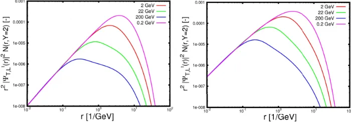
In Fig. 1 we can see the integrand for the structure functionF2(see for example Eq. 9 in [13]) and

its dependence onrforY =2 andY =10. We can see that the interval that contributes the most to the total value ofF2is at aboutr ∼(0.1,20) GeV−1. The highest precision needs to be obtained namely

for these values ofr.

Figure 1. Integrand for the structure function as a function ofrforY =2 (left) andY =10 (right). Each line corresponds to a diﬀerent value of the photon virtualityQ2_.

A signiﬁcant decrease in the running time can be also achieved by modifying the Runge-Kutta method. Since the rcBK evolution equation does not explicitly depend on rapidity, we can split the integration into three terms and then obtain all Runge-Kutta coeﬃcients as their linear combination without the need to recompute the integration itself. The three terms stand as follows [13]

I0=

dr1Krun(r1, r2,r)

I1=

dr1Krun(r1, r2,r)(N(Y, r1)+N(Y, r2))

I2=

dr1Krun(r1, r2,r)(N(Y, r1)N(Y, r2))

(7)

and the Runge-Kutta coeﬃcients can be expressed as

k1 =I1−I2−I0·N(r,Y) (8)

k2 =k1+

1 2hk1I0−

1 2hk1I1−

1 4h

2

k12I0 (9)

k3 =k1+

1 2hk2I0−

1 2hk2I1−

1 4h

2

k22I0 (10)

k4 =k1+

1 2hk3I0−

1 2hk3I1−

1 4h

2

(4)

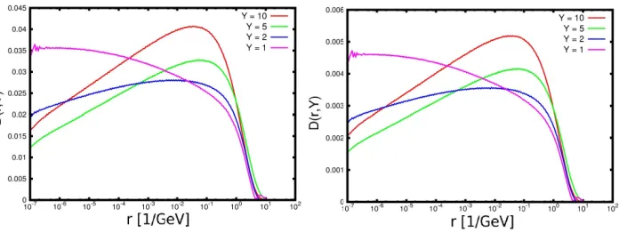
Figure 2. A variation of the Runge-Kutta method. Left - Runge-Kutta method of ﬁrst order compared to the second, right - second order compared to the fourth.

Figure 3.A variation of the rapidity step. Left - step of 0.05 compared to 0.01, right - step of 0.01 compared to 0.005.

4 Results

There is less than 0.7% difference in the rcBK solution when comparing first order Runge-Kutta method to the second order up toY =10 and less than 0.4% for comparing second order to fourth. Therefore, there is less than 1% uncertainty coming from the choice of the Runge-Kutta method and the uncertainty rises with rapidity. Considering the step in rapidity for the Runge-Kutta method, it can be seen that the difference between the step of 0.5 to the step of 0.1 is up to 4% and the biggest difference is in the region where the integrand dominates. Therefore it can be presumed that the uncertainty will also rise with rapidity. The difference between the step of 0.1 to the step of 0.05 is less than approximately 0.5%.

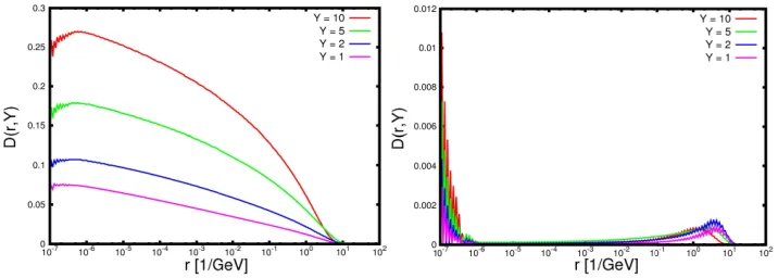
When the variation of the number of steps for the magnitude ofr1 is done from 10 steps to 25

steps per order of magnitude ofr1, the diﬀerence quickly rises with rapidity up to 2.5% atY = 10.

(5)

Figure 4. A variation of the step in integration overr, left - the step of 10 over one order of magnitude ofr1

compared to 25, right - the step of 25 compared to the step of 50.

Figure 5.A variation of the step in integration overθ. Left - the step of 5 over the interval of [0, π] compared to 10, right - the step of 10 compared to the step of 20.

Also, the variation of the number of steps for the angleθbetweenr1andrfrom 5 steps to 10 steps

over the interval [0, π] has been performed resulting in huge diﬀerence up to 25% which quickly rises with rapidity. Adding more steps does not yield to any notable diﬀerence.

Running time for a ﬁxed scale was about 100 s on a regular personal computer and the mean square variation was below 1.5% of the experimentally measured values ofF2.

5 Conclusion

There are several models that predict the eﬀect of saturation of partons in high-energy collisions. Balitsky-Kovchegov evolution equation does that by modifying the BFKL equation with recombina-tion processes that occur in hadrons at high energies.

(6)

The optimal parameters to compute the rcBK equation prove to be: • 25 steps per one order of magnitude ofr,

• 10 steps inθover the interval [0;π], • Runge-Kutta method of fourth order,

• A step of 0.01 in rapidity for the Runge-Kutta method.

Acknowledgment

This work was partially supported by the grant of the Grant Agency of Czech Republic n.13-20841S and by grant LK11209 of MŠMT ˇCR.

References

[1] V.S. Fadin, E.A. Kuraev, L.N. Lipatov, Phys. Lett.B60, 50 (1975) [2] L.N. Lipatov, Sov. J. Nucl. Phys.23, 338 (1976), [Yad. Fiz.23,642(1976)]

[3] E.A. Kuraev, L.N. Lipatov, V.S. Fadin, Sov. Phys. JETP 44, 443 (1976), [Zh. Eksp. Teor. Fiz.71,840(1976)]

[4] E. Kuraev, L. Lipatov, V.S. Fadin, Sov.Phys.JETP45, 199 (1977) [5] I. Balitsky, L. Lipatov, Sov.J.Nucl.Phys.28, 822 (1978)

[6] I. Balitsky, Nucl. Phys.B463, 99 (1996),hep-ph/9509348

[7] Y.V. Kovchegov, Phys. Rev.D60, 034008 (1999),hep-ph/9901281 [8] J.L. Albacete, Y.V. Kovchegov, Phys. Rev.D75, 125021 (2007),0704.0612

[9] J.L. Albacete, N. Armesto, J.G. Milhano, C.A. Salgado, Phys. Rev. D80, 034031 (2009),

0902.1112

[10] J.L. Albacete, N. Armesto, J.G. Milhano, P. Quiroga-Arias, C.A. Salgado, Eur. Phys. J.C71, 1705 (2011),1012.4408

[11] M. Kuhlen, Springer Tracts Mod. Phys.150, 1 (1999)

[12] Y.V. Kovchegov, Phys. Rev.D61, 074018 (2000),hep-ph/9905214 [13] J. Cepila, J.G. Contreras (2015),1501.06687

[14] I. Balitsky, Phys. Rev.D75, 014001 (2007),hep-ph/0609105