Implicit Discourse Relation Recognition by Selecting Typical Training Examples

Implicit Discourse Relation Recognition by Selecting

Typical Training Examples

Xun Wang

Sujian Li

Jiwei Li

Wenjie Li

(1) Key Laboratory of Computational Linguistics, Peking University , M inistry of Education, CHINA (2) Department of Computing, Hong Kong Polytechnic University

{xunwang,lisujian,bdlijiwei}@pku.edu.cn, [email protected]

ABST RACT

Implic it discourse relation recognition is a challenging task in the natural language processing fie ld, but important to many applications such as qu estion answering, summa rizat ion and so on. Previous research used either art ific ially c reated imp lic it discourse relat ions with connectives re moved fro m e xp licit relations or annotated implicit relat ions as training data to detect the possible implic it re lations, and do not further discern which e xa mples are fit to be training data. This paper is the first time to apply a d iffe rent typical/atypical perspective to select the most suitable discourse relation e xa mp les as training data. To differentiate typica l and atypical e xa mples for each discourse relation, a novel single centroid clustering algorithm is proposed. With this typical/atypical distinction, we aim to recognize those easily identified discourse relations more p recisely so as to promote the performance of the implic it re lation recognition. The e xperimental results verify that the proposed new method outperforms the state -of-the-art methods.

KEYWORDS : Discourse relation recognition, single centroid clustering, implic it discourse relation.

1

Introduction

It is widely agreed that sentences/clauses are usually not understood in isolation, but in re lation to their neighbouring sentences/clauses. The task of discourse relat ion recognition is to identify and label the relations between sentences/clauses, wh ich is funda mental to many natural language processing applications such as question answering, automatic summarization and so on. Discourse relations, such as comparison and causal relat ions, can be divided into exp lic it and implic it re lations by the presence or absence of discourse connectives (e.g., but, because et. al.). Previous study indicates that the presence of discourse markers can great ly help re lation recognition and the most general senses (i.e., co mparison, contingency, temporal and expansion ) can be disa mbiguated with 93% accuracy based solely on the discourse connectives (Pitle r et a l., 2008). On the other hand, the absence of exp licit te xtual cues ma kes it very difficult to identify the implicit d iscourse relations. Thus, recently discourse relation recognition research puts more efforts to meet the challenges in implicit discourse relation recognition.

Existing work ma inly focused on explo iting various linguistic features to learn the implic it discourse relation c lassifiers based on the training data collected (We llner, Pustejovsky and Havasi, 2006; Pitler, Louis and Nenkova, 2009; Lin, Kan and Ng 2009; Wang, Su and Tan, 2010). Most useful linguistic features (such as word pairs) a re e xt racted fro m the local context , which is usually determined as Argument 1 (Arg1, the first sentence/clause) plus Argume nt 2 (Arg2, the second sentence/clause). Like the other related work in the literature, in this paper, we focus on the recognition of local implicit discourse relations, i.e. only the two argu ments are examined. To collect tra ining data, the state-of-the-art methods normally start fro m the artific ia l/real perspective and simply ma ke use of the imp licit re lations either derived fro m e xp lic it or manual annotations. Marcu and Echihabi (2002); Sporleder and Lascarides (2008) created artific ial implic it re lations as training data by removing discourse connectives from the exp lic it re lation e xa mples. The advantage of these methods is that a large nu mber of (art ificia l) implic it re lation e xa mples could be used as training data, saving the labor e xtensive and time -consuming annotation work. Ho wever, the e xperimental results in Sporleder and Lascarides (2008) showed that training on a large art ificia l data set is not necessarily a good strategy . Lin, Kan and Ng (2009) a lso pointed out that an artificia lly implic it re lation corpus may e xh ibit marked diffe rences fro m a native ly implic it one. A lso surprising is the fact that the results were not as good as expected when the c lassifiers are tra ined by using the manually annotated real implic it relations, though better than the results based on the artificial implicit relations.

Then the follo wing questions come to our minds. Do all the real natively imp licit re lation e xa mples provide useful hints for training t he classifiers? Is it a reasonable choice if the training data is over-restricted to the annotated implic it re lation e xa mples even when the quantity of these data is limited and their annotation demands a high cost? Can a part of, if not all of, the a rtifi c ial implic it re lations created fro m the e xplic it re lations be picked out to train an implic it re lation classifier? In short, can we obtain more effective training examples at less cost?

an implicit re lation classifie r with higher discrimination power can be built according to the linguistic features in the two arguments.

We provide three Comparison relat ion e xa mp les fro m the Penn Discourse TreeBank (PDTB) v2.0 (Prasad et al., 2008) wh ich is widely used in the research of relation recognition as follows to illustrate what the possible typical examples are like.

(1) Arg 1: 44 North Koreans oppose the plan,

Arg 2: (while) South Koreans, Japanese and Taiwanese accept it or are neutral. (2) Arg 1: In such situations, you cannot write rules in advance.

Arg 2: you can only make sure the President takes the responsibility. (3) Arg 1: Columbia Savings is a major holder of so -called junk bonds.

Arg 2: Ne w federa l leg islation requires that all thrifts divest themselves of such speculative securities over a period of years.

Here, the first one is an art ificia l implic it re lation with the connective (i.e. “while”) deleted wh ile the second and third e xa mples are native ly implic it. The first and second ones are possibly typical because they have distinguishable linguistic features (such as: oppose/accept, cannot /can) to verify their re lations. In contrast, it is hard to find significant cha racteristics in the third one to determine its discourse relation. The trained implicit relation classifier would possibly suffer a decline in performance if a lot of examples like the third one are included in the training set. Based on the analysis above, we for the first time propose to select training data for implic it discourse relation recognition fro m a new typical/atypical perspective other than fro m an artific ial/rea l perspective. Identifying the typical e xa mples fro m both artific ially created and real implic it discourse relations is the focus of this work. Assuming that the typical e xa mples of a discourse relation are usually connected through the similar features, Yaro wsky’s algorithm (1995), as one of the first bootstrapping algorithms, gives us the following inspiration: given a small set of seed typical discourse relation e xa mples, mo re typica l e xa mples are added iterative ly by identifying the significant features of the seed set. In th is paper, a tra ining data selection approach named single centroid c lustering (SCC) is proposed to acquire the typical e xa mp les for each relation. With the typical e xa mp les in the tra ining set, the task of imp licit re lation recognition is cast to a c lassification proble m. The e xpe rimental results show that the train ing set selected in such a way can improve the performance of an implicit relation classifier.

The rest of this paper is organized as fo llo ws. Section 2 introduce s the related work. Sect ion 3 describes our fra mework of imp lic it relat ion recognition, and introduces the types of features involved. Section 4 proposes the single centroid clustering algorith m that selects the typical examples iteratively. Section 5 presents the experimental results. Section 6 concludes our work.

2

Related Work

2.1

Implicit discourse relation recognition

presented by Marcu and Echihabi (2002) who applied massive a mounts of unannotated explic it relations and le xica l features to train the Naïve Bayes classifier for both exp lic it and implic it discourse relation recognition. Following the same idea, Sa ito, Ya ma moto and Se kine (2006) conducted the experiments with the co mb ination of cross -argument wo rd pairs and phrasal patterns as features on Japanese sentences. Bla ir-Go ldensohn (2007) further e xtended the work of Marcu and Echihabi (2002) by involving syntactic filtering and topic segmentation. Another interesting work is that of Zhou et al. (2010), which predicted discourse connectives between arguments via a language model. Then the generated connectives plus other linguistic features were combined in a supervised framework to determine the implicit discourse relation.

However, Sporleder and Lascarides (2008) d iscovered that the models of Marcu and Echihabi (2002) did not perform well on imp lic it re lations recognition with artificia lly created relations as training data and concluded that removing discourse markers may lead to a meaning shift in the e xa mples. Sporleder and Lascarides (2008) p ro moted the other research line that used the human -annotated training data. The develop ment of various discourse banks also made the u se of human-annotated data feasible. Based on Rhetorica l Structure Theory Discourse Treebank (RST-DT) (Carlson et al. 2001), Soricut and Marcu (2003) developed two probabilistic models to identify e le mentary discourse units and generate discourse trees at the sentence level. Further Hernault et al. (2010); Feng and Hirst (2012) e xplo re various features for discourse tree building on RST-DT. With the Discourse Graphbank (Wolf and Gibson, 2005), Wellner et al.(2006) integrated mult iple knowledge sources to produce syntactic and lexica l semantic features, which were then used to automatically identify and classify e xp lic it and imp licit d iscourse relations. Especially afte r the re lease of the second version of the PDTB v2.0 (Prasad et al., 2008), more research began to take the advantage of the annotated implic it relat ions for training purpose and were dedicated to e xplo iting various linguistic features in the supervised frame work (Pitler, Louis and Nenkova, 2009; Lin, Kan and Ng, 2009; Wang, Su and Tan, 2010). L in, Kan and Ng (2009) conducted a thorough performance analysis for four c lasses of features including contextual relations, constituent parse features, dependency parse features and cross -argument le xical pairs, while Pit ler et a l. (2009) applied several linguistically informed features, such as word polarity, verb classes, and word pairs. Wang, Su and Tan (2010) adopted the tree kernel approach to mine more structure informat ion and got better results. These efforts of feature selection have achieved better performance though not that satisfying. The quality of tra ining data are partly responsible for the difficulty of improving the performance of implicit relation recognition .

To better recognize the imp lic it discourse relations, we propose to review the annotated discourse corpora available at hand, identify and choose typical re lation e xa mp les as training data for supervised learning. To the best of our knowledge, this paper is the first time to re -thin k the training data and implicit relation recognition from a novel perspective.

2.2

Rhetoric Discourse Treebank and Penn Discourse Treebank

As for the available discourse corpora, due to the space limitation we main ly introduce the two wide ly used discourse corpora - the Penn Discourse TreeBank (PDTB) and Rhetorical Structure Theory Discourse Treebank (RST-DT), which provide a co mmon platfo rm for researchers to develop discourse-centric systems.

e xpressed the relation between the sentences. Then, the annotations can be seen as being of a predicate-argument structure, where a discourse connective is treated as a predicate taking a pair of adjacent sentences as its arguments. Thus, this discourse connective grounded approach e xposes a clearly defined level of discourse structure. In PDTB, a h ierarchy of re lation tags is provided for the re lation annotation. In our e xpe riments, we only use the top level of the annotations, which is composed of four ma jor re lation classes: Temporal, Contingency, Comparison and Expansion. These four core relat ions allow us to be theory-neutral, since they are almost included in all discourse theories, sometimes under different names.

RST-DT is manually annotated under the Rhetoric Structure Theory fra me work (Mann and Thompson, 1988). In this corpus the rhetoric re lations are labe lled hiera rchica lly between non-overlapping adjacent te xt spans which range fro m e le mentary d iscourse units (EDU, the minimal building blocks of a discourse tree) to paragraph. A total of 110 diffe rent relations were used for the tagging of the RST corpus (RST -DT, 2002). The fina l inventory of the relations is data driven and can be partitioned into 18 c lasses , fro m which we still select four c lasses including Temporal, Contrast, Cause, and Background to verify our method. These four relations spanning over individual sentences are collected to keep consistent with the discourse relations from PDTB. So far, most of the previous works experimented on one corpus only. With the aim to verify the portability of our methods, we examine two corp ora in this paper.

3

The Learning Framework for Implicit Discourse Relation Recognition

In this paper, the problem of implic it relat ion recognition is approached in the supervised learning framework. Figure 1 illustrates the architecture of our system.

The first and most important step is to collect the tra ining data. As stated in Section 1, on the one hand, not all the annotated implic it re lations contain significant features to distinguish themselves fro m the other relat ion types. On the other hand, we e xp ect to pick out the suitable exa mp les of the artific ial implic it relat ions and strengthen their influence on the tra ining process. We argue that the exa mples suitable to be training data are genera lly the typical ones having distinct linguistic features to signify their discourse relations, yet they can be of real implic it re lations (denoted as IM data) or art ificia lly imp lic it relat ions with connectives removed fro m e xplic it relations (denoted as EX data).

To select typical e xa mp les, for each discourse relation type the original a rtific ial/ real part ition (denoted as EXi/IMi) is converted to a novel typica l/atypical part ition (denoted as Ai/Bi), which is obtained automatica lly by the proposed single centroid clustering (SCC) a lgorith m. Start ing fro m an initia l seed set, SCC iterat ively re fines typical e xa mples and re moves atypical e xa mp les if necessary. This algorithm is detailed in Section 4.

FIGURE 1

–

Assume there are n discourse relations. Let Y={R0, R1,…, Rn} where Ri represents the ith typical relation type and R0 denotes the atypical case. After the conversion fro m a rtific ial/ real partit ion to

Training data Selection Discourse

corpus

EXiIMi Classifier

Training Model Discourse

typical/atypical partition, we get the Ai/Bi(1≤i≤n) and assign the relation label Ri(1≤i≤n) to each typical e xa mp le in the set Ai. Each e xa mp le in the union A0=∪Bi(1≤i≤n) is labelled as R0. Then the set of ordered pairs <Ai, Ri> (0≤i≤n) can be used to train an implicit relat ion classifier for labelling Ri(1≤i≤n). Both clustering and c lassification require representing the annotated argument pairs with feature vectors. We introduce the feature selection in subsection 3.1.

3.1

Feature Selection

Various linguistic features have been e xperimented for recognizing imp licit discourse relations in previous studies (Marcu and Echihabi, 2002; Pit ler, Lou is and Nenkova, 2009; Lin et al., 2009). Learning from them, we consider the following 7 types of features.

Polarity: The polarity of each s entiment word is tagged as positive, negative or neutral according to Multi-perspective Question Answering Op inion Co rpus (Wilson et al., 2005). Note that the sentiment words preceded by negated words would be assigned an opposite tag. For e xa mple , "good" would be assigned as positive while “not good” is negative. Negated neutral is ignored. The occurrence of negative, positive and neutral polarities in each argu ment and their cross product are used as features.

Inquirer tags: Genera l Inquirer le xicon (Stone et al., 1966) divides e ach word into fine-g rained semantic categories described by the inquirer tags. Fro m all the categories, we select 21 pa irs of comple mentary categories, such as: Rise versus Fall, or Pleasure versus Pain, etc. The occurrence of each complementary category p air in the two arguments are used as features.

Modality: The presence of modal words inc luding their various tenses and abbreviations in both arguments and their cross product are used as features.

SameWor d: This type of feature represents whether a noun or a verb simultaneously occurs in

both arguments. The intuition of using this feature is similar to that of the Verbs feature in (Pitler et al., 2009), for indicating the semantic association of the two arguments.

FirstLastFirst3: The first word, the last wo rd, the first three words of each argu ment, the pair of the two first words and the pair of the two last words in thetwo arguments are used as features.

CrossWor dPairs: The words in each argument compose one set. This type of features indicates

the word pairs from the cross product of the two sets.

IntraWordPairs: The word pairs that occur in the same argument.

Since the length of the two arguments is relat ively short, it is quite co mmon that a feature is observed only once if it is present. Hence each feature is assigned a binary value to indicate whether it is present or absent. Assuming d features are e xtracted, each e xa mp le is represented with a d-dimension binary feature vector.

4

Single Centroid Clustering for Training Example Selection

4.1

Overview

we introduce the Single Centroid Clustering (SCC) algorith m wh ich pic ks out the typical examples for each discourse relation from both EX and IM data.

Algorithm 1: Single-Centroid Clustering algorithm

Input: For relat ion i, a rtific ial implic it re lation set EXi, real implicit relation set IMi,

Output: Typical relat ion e xa mp le set Ai, Atypical relation example set Bi

1. Initialize Ai: Ai= seed set of typical examples ; 2. Bi= EXi∪IMi-Ai

3. Compute the centroid CAi for Ai 4. While stopping criterion has not been met 5. For each example ej in Ai:

6. If dist (ej, CAi) > :

7. Ai = Ai - {ej}; Bi = Bi∪{ej} 8. For each example ej in Bi: 9. If dist(ej, CAi)<= : 10. Ai= Ai∪ {ej}; Bi = Bi - {ej} 11. Compute the centroid CAi for Ai 12. End While

FIGURE 2

–

Figure 2 illustrates a snapshot of SCC on re lation Ri, with dots and crosses representing the data in the Ai and Bi sets respectively. The c losed curve in the le ft-top graph represents the seed set of typical e xa mp les. The closed curves in the other three graphs represent the intermediate and final results of the typical e xa mples sets. The solid triangles in the middle of the closed curves denote the centroids computed based on typical e xa mples. When SCC reaches its stable state, the final typical e xa mp le set is passed to the classification models as train ing data. Take the three sentence pairs in Section 1 for e xa mple, the ideal outpu t from SCC should include the first and the second examples in the typical set of the Comparison relation.

4.2

Implementation Details

4.2.1 Seed Set Construction

For each re lation Ri(1≤i≤n), we can identify a re latively sma ll number of typical e xa mples as the seed set either manually or automat ically. Simila r to the Yarowsky a lgorith m (1995), to avoid the laborious procedure, through observation we manually lay down some simp le rules toidentify the distinct features for each relation from the 7 feature types and then select those containing the distinct features from the corresponding relation e xa mp les to compose of the seed set. The rules for identifying distinct features are illustrated in Table 1. Taking the Comparison relation for e xa mple , rule (1) identify the features of “Arg 1 is positive and Arg 2 is negative” and “Arg 1 is negative and Arg 2 is positive” which a re fro m the Polari ty feature type. Rule (2) can identify the features which a re related to the words seldom, back, etc. accord ing to the feature types of

FirstLastFirst3, Cr ossWordPairs, and Intr aWor dPairs. Other strategies of selecting typical example seed set and the experimental comparisons are provided in Subsection 5.3.

Class Description of Rules

Comparison (1) A pair of opposite polarity tags is identified respectively in Arg 1 and Arg 2. _{(2) Arg 1 or Arg 2 contains the words including seldom, back, yet,only.}

Contingency (1) Opposite polarity tags are identified respectively in Arg 1 and Arg 2. (2) Arg 1 or Arg 2 contains the words including draw, as, result. Temporal Arg 1 or Arg 2 contains the words including following, last, first, second. Expansion Arg 1 and Arg 2 contain the same noun words or verb words.

TABLE 1– Rules for selecting the seed set of typical examples .

4.2.2 Centroid Computati on

Ai can be seen as the iteratively re fin ed typical set. Suppose Ai is composed of |Ai| e xa mples , each e xa mp le (1≤j≤|Ai|) is represented by a d-dimension feature vector In the d-d imensional Boolean space, the centroid CAi is a lso represented by a d-dimension binary feature vector , where is the value in the kth _dimension. We define as:

{

∑

In this way, the centroid values actually re flect which features are significant to the corresponding discourse relation. Norma lly, centro id is used to compute the “average” of a ll objects in a certain space, and it should be noted that the computation of centroid in a Boolean space here does not strictly observe the “average” form.

4.2.3 Distance Metric

For each relation Ri, we e xc lude atypical exa mp les fro m Ai or select typical ones into Ai by computing the distance between discourse relation e xa mp le s and the centroid of CAi. Assuming the e xa mple e is represented by the feature vector (e1, e2, …,ed), the d istance between e and CAi is defined as follows.

∑ (2)

{

∑

∑

(3)

where reflects whether the e xa mple e has a diffe rent value fro m CAi in the k-th dimension and wk (1≤k≤d) is used to measure the influence of the difference in the k-th dimension on the distance between e and CAi. He re, wk is determined according to the frequency of the k-th feature occurring in a ll e xa mples of a discourse relation. The d istance between an e xa mp le e and the centroid CAi denotes the representativeness or to say the typicality of the e xa mple e to the relation Ri. The smaller the distance value of an example, the more typical the example is. A distance threshold

is set to control which e xa mples should be selected into the typical set of Ri. The e xa mples with distance less than are possibly re-assigned to the typical set Ai. is defined depending on the ma ximu m d istance and the minimu m d istance between the e xa mples and the centroid CAi, i.e.,

₍₄₎

where p(i) _{is a control para meter with in the interval (0,1) fo r Ri. If p}( i) _{is set 0,}

equals to the minimu m d istance, meaning that no e xa mples can be included into the typical set. On the other e xtre me, if p( i) _{is 1,}

equals to the ma ximu m d istance, it allows all the e xa mples to be selected. The value of p(i) _{is also tuned to assure that typical e xa mp les can be well selected in each iteration.}

5

Experiments and Evaluation

5.1

Experiment Set-up

sentence pair to be annotated with more than one relation, we only e xtract the first relation labelled for each sentence pair here. Table 2 shows the number of each relations in PDTB.

Class Training Test Develop.

EX IM Implicit Implicit

Comparison 4209 1894 146 191

Contingency 2505 3281 277 287

Temporal 2633 665 67 54

Expansion 4770 6792 556 651

Total 14117 12632 1046 1183

TABLE 2– Discourse relation distribution in PDTB.

According to the 7 types of features introduced in Section 3.1, in total 4022 features are e xtracted. Then each sentence pair is represented as a 4022-d imension binary feature vector. The two classifie rs, i.e., the Naïve Bayes and Dec ision Tree classifie rs are imp le mented with MALLET1_{. Two metrics, i.e., accuracy and F}

1 measure, are used to evaluate the performance:

and

where precision and recall are two most co mmon c riteria to evaluate informat ion retrieval and

information extraction systems.

Four sets of experiments are designed (1) to tune the two thresholds and

in SCC; (2) to compare different strategies of selecting seed sets for SCC; (3) to co mpare the performance of various training sets on different classifiers; (4) to verify th e portability of our methods.

5.2

Threshold Tuning in SCC

SCC a ims at selecting typical e xa mples for tra ining discourse classifiers. Since it is difficult to directly evaluate the quality of a train ing set, we evaluate the training set outputted by SCC via the classification performance of a Dec ision Tree classifie r. For each discourse relation Ri, SCC involves two ma in thresholds. determines wh ich features are significant to the re lation Ri, and

defines the borderline between the typical e xa mples and the atypical ones. It is hard to find a global optimized solution for the co mb ination of these two factors. So we apply a gradient search strategy. As in formu la (4), p(i) _{is the only determin ing factor of}

. At first we set p(i) _{the value of 0.5, and different values of ranging fro m 0.05 to 0.35 are e xa mined.} Then, given that is set to the value with the best performance, we conduct experiments to find an appropriate value for p(i)_.

We ran four binary classifiers to distinguish each discourse relation (Co mp., Cont., Te mp., and Expa. for short) fro m the others. For each re lation, we include equal nu mber of positive and negative e xa mples in the tra ining data. The positive e xa mples a re selected fro m the typical set of the relation wh ile the negative e xa mples are randomly chosen from the atypical set of the same relation or the other discourse relations. We use all the 1183 imp licit re lations in the development set, which is representative of the natural d istribution of imp licit discourse relations. Table 3 lists the F1 and accuracy (within parentheses ) of the implicit relation classifiers.

Tc Comp. vs. other Cont. vs. other Temp. vs. other Expa. vs. other

0.05 23.2 (54.2) 39.0 (24.3) 12.8 (54.5) 0 (45.0)

0.10 23.9 (40.4) 41.9 (26.5) 12.8 (46.4) 64.4 (53.6)

0.15 27.9 (39.4) 38.6 (24.6) 12.5 (43.6) 66.2 (54.6)

0.20 27.6 (24.1) 39.9 (37.4) 12.4 (47.1) 68.3 (55.4)

0.25 17.4 (75.1) 42.1 (29.1) 13.4 (45.5) 71.0 (55.0)

0.30 18.4 (73.0) 42.3 (28.3) 11.7 (45.2) 55.2 (50.0)

0.35 17.0 (74.9) 39.1 (24.8) 12.6 (43.0) 55.2 (50.0)

TABLE 3–F1 (Acc) with varying values (p=0.5).

Table 3 shows that the value of directly influences the quality of the generated training set. When is assigned a smaller value, more features will satisfy the percentage require ment. That means more features will be re flected in the centroid and it will cause the distance between an exa mp le and the centroid is closer to one another. Then when

is fixed, more e xa mp les will enter into the typical set. Oppositely, when is assigned a la rger va lue, it is more difficult for a feature to satisfy the percentage require ment. Then less number of features is re flected in the centroid. Notice that in general cases when the value of is larger than 0.35, the generated centroid closely approaches to the zero vector and thus does not work in the typical e xa mple selection. According to the best F1 of each relation, we set the values to 0.15, 0.3, 0.25 and

0.25 for Comp., Cont., Temp., and Expa. respectively.

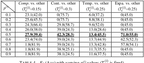
p(i)

Comp. vs. other ( =0.15)

Cont. vs. other ( =0.3)

Temp. vs. other ( =0.25)

Expa. vs. other ( =0.25)

0.1 23.1(42.0) 0(75.7) 6.0(37.2) 0(45.0)

0.2 25.6(45.5) 0(75.7) 8.8(38.1) 0(45.0)

0.3 24.3(66.4) 29.8(58.7) 9.6(52.0) 0(45.0)

0.4 26.0(38.0) 39.0(24.3) 13.0(28.6) 0(45.0)

0.5 27.9(39.4) 42.3(28.3) 13.4(45.5) 71.0(55.0)

0.6 23.4(74.0) 39.0(24.3) 13.7(44.9) 62.5(52.3)

0.7 1.8(81.9) 39.0(24.3) 13.3(42.8) 57.8(54.1)

0.8 1.8(81.9) 38.9(25.1) 11.7(35.5) 0(45.0)

0.9 1.8(81.9) 38.1(24.5) 11.6(37.5) 0(45.0)

TABLE 4–F1 (Acc) with varying p(i) values ( is fixed). Ne xt, with the tuned values, we inspect the performance of SCC with different

richer linguistic features are involved to indicate the implic it discourse relations. For this reason, the real implicit examples tend to be typical.

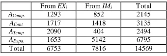
From EXi From IMi Total

AComp. 1293 852 2145

ACont. 1717 1418 3135

ATemp 2090 404 2494

AExpa. 1653 5142 6795

Total 6753 7816 14569

TABLE 5– Constituents of the final typical sets.

5.3

Influence of Initial Seed Sets

The SCC algorithm begins with a seed set of typical e xa mples that are p icked out fro m the training data according to the manually summarized rules (denoted as the manual strategy) in section 4.2.1. The seed sets are generally composed of 1-5% of the corresponding relations.

stragegy Comp. vs. other Cont. vs. other Temp. vs. other Expa. vs. other

M anual 27.9(39.4) 42.3(28.3) 13.7(44.9) 71.0(55.0)

IM_seed 22.5(57.6) 39.8(47.4) 9.5(48.5) 50.9(47.4)

EX_seed 20.2(62.6) 39.0(24.3) 7.9(45.0) 55.2(50.0)

Random 19.1(75.7) 37.8(29.8) 8.0(27.9) 53.6(45.2)

TABLE 6–F1 (Acc) with different seed sets on Dev. Data.

stragegy Comp. vs. other Cont. vs. other Temp. vs. other Expa. vs. other

M anual 28.5(62.0) 48.5(49.4) 14.7(69.0) 71.1(57.3)

IM_seed 26.4(60.7) 41.9(26.5) 12.0(35.8) 52.6(49.2)

EX_seed 21.2(63.0) 41.9(35.4) 11.7(52.4) 54.6(50.1)

Random 22.2(47.1) 36.3(48.8) 11.1(40.2) 52.6(49.2)

TABLE 7–F1 (Acc) with different seed sets on Test Data.

For co mparison purpose, we also e xa mine the other three automatic seed set selection strategies on both development and test data. The results are shown in Table 6 and Table 7. We select the IM and EX data as seed set separately, denoted as IM_seed and EX_seed strategy respectively. With the Rando m strategy, we randomly select 10% of e xa mp les fro m the EX and IM data as the seed set for each relation. Both Table 6 and Table 7 show the superiority of the manual strategy over the other three. SCC to some e xtent is sensitive to the init ialization o f the typica l set and could achieve a better performance with a better seed set of typical examples .

5.4

Evaluation of Implicit Relation Classifiers

Pit ler’s best results using single feature (Pitle r-1) and co mbined features (Pitle r-2), which are evaluated by a Naïve Bayes classifier. The IMi, EXi, EXi+IMi rows refer to our results of directly taking the IM data, the EX data, and both the EX and IM data as the training set respectively. Notice that all imp le mentation of the IMi method but feature selection is the same as Pitler’s, though the performance of the IMi method is fa r belo w Pit ler’s best results. This means feature selection is a key to promoting the performance.

Comp. vs. Other

Cont. vs. Other

Temp. vs. Other

Expa. vs.

Other 4-way

NB

Pitler-1 21.0(52.6) 36.7(62.4) 15.9(61.2) 71.3(59.2) (65.4)

Pitler-2 22.0(56.6) 47.1(67.3) 16.8(63.5) 76.4(63.6)

--IMi 6.7(81.4) 41.9(28.0) 13.4(30.7) 44.4(51.9) (51.3)

EXi 18.7(74.3) 40.1(27.6) 12.4(48.6) 8.2(46.6) (34.1)

EXi+IMi 14.0(76.5) 41.9(27.0) 12.7(44.8) 27.5(47.5) (42.3) SCC 24.3(58.3) 43.1(65.2) 18.0(92.2) 68.6(52.4) (68.3)

DT

IMi 11.6(41.5) 38.7(40.5) 14.3(76.1) 38.8(44.7) (53.5)

EXi 18.9(70.5) 41.9(26.5) 12.1(8.2) 0(46.8) (42.6)

EXi+IMi 14.0(76.5) 41.9(26.5) 9.0(67.3) 0(46.8) (51.4)

SCC 28.5(62.0) 48.5(49.4) 14.7(69.0) 71.1(57.3) (72.2)

TABLE 8– Performance comparison on PDTB.

SCC means using the training set which is composed of typical exa mp les. Since the typical e xa mples are p icked out by SCC due to their distinct features, it is more suitable for the DT classifier to acquire the classifying rules according to the distinct features. Th at is why the performance of the DT c lassifier is better than that of the NB classifier in Table 8. The performance of both the DT and NB classifie rs trained by typical e xa mp les are comparable to Pit ler-1 and Pitle r-2, though feature selection is not concerned in our systems. This table also shows that using typical e xa mp les as training data is more effective than using either IMi, EXi, or both IMi and EXi data as training set. For detecting the comparison relation with the DT c lassifier, the training set output by SCC significantly outperforms IMi, by as much as about 17% absolute improve ment in F1-scores (i.e., 28.5 vs. 11.6). It is also observed that the performance of using IMi as train ing set is co mparable to that of using EXi. Th is conforms to our assumption that typical e xa mp les contributes to the classification perfo rmance , while the fina l typical e xa mp le set is composed of almost the same percent of the IM data and EX data according to Table 5. According to the typical/atypical distribution in the train ing data , the test data should be composed of about 61.8% of typica l ones and 38.2% of atypical ones. Since we do not preprocess the test data, the typical e xa mples and the atypica l ones in the test data are identified for their relations simultaneously. We observe the 4-way classification results with the DT class ifie r and find that most exa mp les correctly identified a re typical wh ile the wrong ly identified e xa mp les are usually atypical. For example, the third example in Section 1 is identified as Expansion.

5.5

Evaluation of Portability

the 4 discourse relations spanning over individual sent ences. Table 9 illustrates the relation distribution. For the 4 relations, we set = 0.25 and p(i)_{=0.5, SCC outputs the typical and} atypical sets and their sizes are also given in the table.

Class Training Test SCC

EXi IMi Implicit Ai Bi

Contrast 972 578 311 610 940

Background 701 677 330 660 718

Cause 304 785 535 846 243

Temporal 466 462 244 590 338

TABLE 9– Relation distribution on RST.

Here, we evaluate the perfo rmance of SCC with the Dec ision Tree c lassifier. We co mpare it with the three baselines: real implic it e xa mp les (IMi), a rtific ia l imp licit e xa mp les (EXi) or all the e xa mples as train ing data (IMi+EXi). Table 10 shows that SCC can pro mote the performance with statistical significance (i.e., p-value2_{<0.1) on F1. In addition, F1 of Contrast vs Other (31.6)} outperforms that of Comparison vs Other (28.5) on PDTB. It is the same for Temporal. According to our analysis , the reason is that the relations of RST-DT are fine-gra ined and it is relatively easy for SCC to obtain typical examples.

Contrast vs. Other Background vs. Other Cause vs. Other Temporal vs. Other

SCC 31.6 (43.3) 38.3 (31.1) 54.8 (37.7) 31.2 (38.2)

IMi 27.6 (56.1) 34.8 (30.4) 35.6 (54.4) 29.2 (17.1)

EXi 24.0 (64.9) 34.0 (41.5) 30.6 (57.1) 17.6 (67.0)

IMi+EXi 20.8(62.4) 34.9 (30.5) 32.2 (56.6) 27.2 (43.8)

TABLE 10–F1 (Acc) comparison on RST-DT.

Conclusions

In this paper, we for the first time present the typical/atypical perspective to select the most suitable training e xa mp les for imp licit discourse relation recognition. A novel single centroid clustering algorithm is proposed to differentiate typical and atypical e xa mples for each discourse relation. The e xperimental results show that the performance of the imp lic it re lation classifiers with the typical e xa mp les selected as the training set are co mparable to the best state -of-the-art methods on PDTB v 2.0. In addition, the experiments on RST-DT show statistically significant improve ments over the baselines and demonstrate the portability of our method. We will further e xplore mo re linguistic features and employ our approach on finer gra ined re lation types. In SCC, we want to further investigate other distance formu la. We also hope to exp lore the effective way to make use of the unlabelled discourse data.

Acknowledgments

The research work described in this paper has been partially supported by NSFC grants (No.61273278 and No.90920011), NSSFC grant (No : 10CYY023), National Key Technology R&D Progra m (No : 2011BAH10B04-03), and Nat ional High Technology R&D Progra m (No. 2012AA011101). We also thank the three anonymous reviewers for their helpful comments.

References

Carlson, L., Marcu, D. and Okuro wski, M.E. (2003). Bu ild ing a discourse-tagged corpus in the fra me work of rhetorica l structure theory. In Janvan Kuppelvelt and Ronnie Smith, editors, Current Directions in Discourse and Dialogue. Kluwer Academic Publishers.

Christiann, V. W. and Barnard., E. (2006). Data characteristics that determine c lassifie r performance. In Proceedings of the Sixteenth Annual Symposium of the Pattern Recognition Association of South Africa, pp. 166–171, Parys, South Africa.

Feng, V. W. and Hirst, G., (2012). Te xt -leve l discourse parsing with rich linguistic features, In Proc.of ACL'12, pages 60-68.

Hernault, H., Prendinger, H., David, A., and Mitsuru I. (2010). HILDA: a discourse parser using support vector machine classification. Dialogue and Discourse, 1(3):1-33.

Lin, Z., Kan, M.– Y., and Ng, H. T. (2009). Recognizing imp lic it d iscourse relations in the Penn discourse treebank, In Proceedings of the 2009 Conference on Empirical Methods in Natural Language Processing, Singapore.

Mann, W. C. and Tho mpson, S. A. (1988). Rhetorica l structure theory: towards a functional theory of text organization. Text, 8(3):243-281.

Marcu, D. and Ech ihabi, A. (2002). An unsupervised approach to recognizing d iscourse relations. In Proc. of ACL 2002, pages 368-375.

Pit ler, E., Raghupathy, M., Mehta, H., Nenkova, A., Lee, A. and Joshi, A. (2008). Easily identifiable d iscourse relations. In Proc. of the 22nd International Conference on Computational Linguistics (COLING08). pages 85-88.

Pit ler, E., Louis, A. and Nenkova, A. (2009). Automatic sense prediction for implicit d iscourse relations in text, In Proc. of the 47th ACL. pages 683-691.

Prasad, R., Dinesh, N., Lee, A., Miltsakaki, E., Robaldo, L., Joshi, A. and Webber, B. (2008). The Penn discourse treebank 2.0. In Proc. o f the 6th International Conference on Language Resources and Evaluation (LREC). Marrakech, Morocco.

RST_ DT. (2002). RST Discourse Treebank. Linguistic Data Consortium, http://www.ldc.upenn.edu/Catalog/CatalogEntry.jsp?catalogId=LDC2002T07

Saito, M., Ya ma moto, K. and Sekine, S. (2006). Using phrasal patterns to identify discourse relations. In Proc. of the HLTCNA Chapter of the ACL. pages 133-136.

Sasha B.-G. (2007). Long-Answer Question answering and rhetorica l-se mantic re lations. Ph. D. thesis, Columbia Unversity.

Soricut, R. and Marcu, D. (2003). Sentence level discourse parsing using syntactic and le xica l information. In Proc. of HLT/NAACL 2003. pages 149-156.

Sporleder, C. and Lascarides. A. (2008). Using automatica lly labelled e xa mp les to classify rhetorical relations: An Assessment. Natural Language Engineering, 14:369-416.

Wilson, T., W iebe, J. and Hoffmann, P. (2005). Recognizing contextual polarity in phrase-leve l sentiment analysis. In Proc. of the conference on Human Language Technology and Empirical Methods in Natural Language Processing, pp. 347-354.

Wellner, B., Pustejovsky, J., Havasi, C., Ru mshisky, A. and Sauri, R. (2006). Classification of discourse coherence relations: an exploratory study using multip le knowledge sources. In Proc. of the 7th SIGDIAL Work shop on Discourse and Dialogue. pages 117-125.

Yarowsky, D. (1995). Unsupervised word sense disambiguation rivaling supervised methods, In Proc. of the 33rd annual meeting on Association for Computational Linguistics, pages 189-196, Cambridge, Massachusetts.