Selected Topics in Statistical Computing.

(1)

ABSTRACT

ZHANG, YIWEN. Selected Topics in Statistical Computing. (Under the direction of Dr. Hua Zhou.)

As the connection between statistical models and the real data, optimization methods

draw attentions from both academia and industries. Since advances in technology enable

easier data collection, complex models are in demand to cope with data that have

com-plex structures; efficient optimization methods are needed to perform analysis on large

and ever-growing volumes of data. In this dissertation, we investigate the optimization

methods that target at these two issues. The first half of the thesis focuses on

develop-ing and implementdevelop-ing optimization algorithms for multivariate generalized linear models

(MGLM), while the second half addresses the problems with large data sets.

Data with multivariate count responses frequently occur in modern applications. The

commonly used multinomial-logit model is limiting due to its restrictive mean-variance

structure. For instance, analysis of count data from the recent RNA-seq technology by

the multinomial-logit model leads to serious errors in hypothesis testing. The ubiquity

of over-dispersion and complex correlation structures among multivariate counts call for

more flexible regression models. In this dissertation, we study some generalized linear

models with multivariate count responses that incorporate various correlation structures

among the components of the response vector. Current literature lacks treatment of

these models, partly due to the fact that they do not belong to the natural exponential

family. We derive stable optimization algorithms under the minorization-maximization

(MM) principle. Parameter estimation, testing, and variable selection for these models are

treated in a unifying framework. The regression models are compared on both synthetic

(2)

Traditional iterative optimization algorithms require the whole data set to be

avail-able in memory for each iteration. When analyzing large data sets, this optimization

scheme makes the computation sensitive to the memory limit. We investigate the online

optimization algorithms that provide elegant solutions to the analysis on large data sets.

Instead of keeping the whole data set in memory, online algorithms only keep a small

batch of data points in memory at each iteration, and process every data point once. We

(3)

(4)

Selected Topics in Statistical Computing

by Yiwen Zhang

A dissertation submitted to the Graduate Faculty of North Carolina State University

in partial fulfillment of the requirements for the Degree of

Doctor of Philosophy

Statistics

Raleigh, North Carolina

2014

APPROVED BY:

Dr. Eric Laber Dr. Lexin Li

Dr. Brian Reich Dr. Hua Zhou

(5)

DEDICATION

(6)

BIOGRAPHY

The author was born in Fushun, China. She got her bachelor’s degree from Shanghai

Uni-versity of Finance and Economics, majoring in Economics, and minoring in Accounting.

In the year 2009, she enrolled in the master’s program in North Carolina State

Univer-sity Department of Statistics where she switched to the Ph.D. program a year later. She

(7)

ACKNOWLEDGEMENTS

I would like thank my advisor, Dr. Hua Zhou, for his endless patience and constant

help. There is no way I can finish my projects without his input. I have the highest

regard for his passion in research and knowledge in statistics. He has brought me the

inspiration and opened my horizon. When obstacles show up, being cynical is easy, while

staying positive and gathering the self delusion to work on where others have failed,

is not. My advisor’s genuine curiosity and optimism have illuminated our research; his

persistence and integrity have propelled us moving forward. Other than research, it is

very rewarding to work with Dr. Hua Zhou. When he spent tireless efforts helping me

revise my dissertation and was not willing to settle for any imperfection, he demonstrated

the standard he lives by. That is also the standard I want to live up to. There is a lot

more beyond intelligence that I need to earn the degree, as well as all the glory comes

with it. I am blessed to have such an adviser.

I can not make this far without the faculty and staff at North Carolina State.

Espe-cially, I want to express my gratitude to Dr. Pam Arroway for believing in me, encouraging

me, and finding me funding opportunities. I appreciate the research assistantship

posi-tion that Dr. Sharon Schulze offered me. That posiposi-tion gave me precious opportunities

to explain statistical results to non-statisticians, which became an important part of the

training that I could not get in the classroom. I also want to thank Dr. Jackie

Hughes-Oliver, Dr. Sujit Ghosh, Dr. John Monahan, Dr. Kim Weems, and Dr. Howard Bondell

for taking care of all the paperwork, making sure that I make choices that serves the

most benefit to my long-term career. I also want to thank Alison McCoy for her

hart-warming smile. I want to give special thanks to my Ph.D. committee members, Dr. Eric

(8)

given by these brilliant professors encouraged me to be critical to my research topic, to

be meticulous in the research process, and to make better presentation of my research

results. Improvements can not be achieved without their input.

I am also thankful to the opportunity to work at BD Technologies. My manager,

Elaine McVey, gave me invaluable advices on how to be a good statistical consultant.

She showed me the energy and insights a statistician can bring to a project. She provided

me the freedom to explore interesting methodologies and tools. I also want to thank my

co-workers, Yongji Fu, Steven Keith, Frances Tong, and Perry Haaland for making my

internship experience fruitful and memorable.

Finally, I want to thank all my family and friends for their unconditional love and

supports. My parents have always been caring and understanding, even though me being

in another country makes it hard on them. I am grateful that they keep their concerns to

themselves and let me do whatever I want. I am blessed to have the friend who is always

ready to provide consolation, fix bad days, and clear my uncertainties. The emotional

(9)

LIST OF TABLES

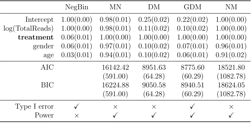
Table 3.1 Example of an RNA-seq data set. . . 44 Table 3.2 Empirical rejection rates for testing each predictor in the simulated

RNA-seq data. The boldfaced predictortreatment has non-zero effect on the exon expression counts. Gender and age have no effects on the expression counts. Numbers in the brackets are standard errors based on 300 simulation replicates. . . 46 Table 3.3 Generalized linear models for multivariate categorical responses. d:

di-mension of response vector;p: number of predictors in regression mod-els;m: the batch size|y|=P

jyjof the response vectory= (y1, . . . , yd);

|α|=P

jαj. . . 47

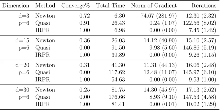
Table 3.4 Comparison of Newton, Quasi-Newton (BFGS), and IRPR methods for fitting Dirichlet-multinomial (DM) regression. Numbers in parenthesis are standard errors based on 100 simulation replicates. . . 80 Table 3.5 Empirical type I error and power of the Wald test by the multinomial

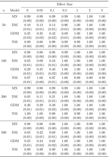
(MN), Dirichlet-multinomial (DM), generalized Dirichlet-multinomial (GDM), and negative multinomial (NM) regression models, based on 500 simulation replicates. Responses are generated from the multinomial (MN) model. Numbers in parenthesis are standard errors. . . 97 Table 3.6 Empirical type I error and power of the Wald test by the multinomial

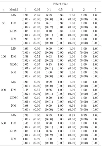
(MN), Dirichlet-multinomial (DM), generalized Dirichlet-multinomial (GDM), and negative multinomial (NM) regression models, based on 500 simulation replicates. Responses are generated from the Dirichlet-multinomial (DM) model. Numbers in parenthesis are standard errors. 98 Table 3.7 Empirical type I error and power of the Wald test by the multinomial

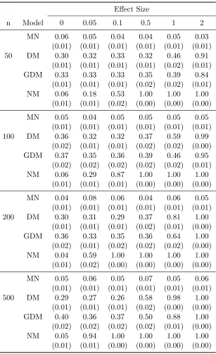
(MN), Dirichlet-multinomial (DM), generalized Dirichlet-multinomial (GDM), and negative multinomial (NM) regression models, based on 500 simulation replicates. Responses are generated from the general-ized Dirichlet-multinomial (GDM) model. Numbers in parenthesis are standard errors. . . 99 Table 3.8 Empirical type I error and power of the Wald test by the multinomial

(12)

Table 3.9 Summary of mean AUCs from the group-penalized estimation by the multinomial (MN), multinomial (DM), generalized Dirichlet-multinomial (GDM) and negative Dirichlet-multinomial (NM) regression models, based on 300 simulation replicates. Responses are generated from the multinomial (MN) model. Standard errors are presented in the paren-thesis. . . 104 Table 3.10 Summary of mean AUCs from the group-penalized estimation by the

multinomial (MN), multinomial (DM), generalized Dirichlet-multinomial (GDM) and negative Dirichlet-multinomial (NM) regression models, based on 300 simulation replicates. Responses are generated from the Dirichlet-multinomial (DM) model. Standard errors are presented in the parenthesis. . . 107 Table 3.11 Summary of mean AUCs from the group-penalized estimation by the

multinomial (MN), multinomial (DM), generalized Dirichlet-multinomial (GDM) and negative Dirichlet-multinomial (NM) regression models, based on 300 simulation replicates. Responses are generated from the generalized Dirichlet-multinomial (GDM) model. Standard errors are presented in the parenthesis. . . 110 Table 3.12 Summary of mean AUCs from the group-penalized estimation by the

multinomial (MN), multinomial (DM), generalized Dirichlet-multinomial (GDM) and negative Dirichlet-multinomial (NM) regression models, based on 300 simulation replicates. Responses are generated from the negative multinomial (NM) model. Standard errors are presented in the parenthesis. . . 113 Table 3.13 SNP signals on Chromosome 8 from eQTL analysis of ST13P6 by GDM

regression. . . 117

(13)

LIST OF FIGURES

Figure 2.1 Histogram of the 524 proportions in the Haseman and Soares data with a Beta(1.23,12.46) density imposed. . . 22 Figure 2.2 Graphs of minorization inequalities (2.9) and (2.10). . . 28 Figure 2.3 Algorithmic iterates for the HS76-1 data set. Left: Start from a blind

guess α(0) _{= (1}_,_{1). Right: Start from the method of moment estimate}

α(0) = (0.4711,4.8072). . . 30 Figure 2.4 Distance of algorithmic iterates to the final solution kθ(t)₋_θ∞_k

2 for

the HS76-1 data set. . . 32 Figure 2.5 Log-likelihood surface and the minorizing functions of EM, MM, and

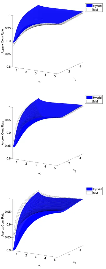
the EM-MM hybrid algorithms at point (0.5,5) for the HS76-1 data set. 33 Figure 2.6 Approximate convergence rates of the MM and hybrid algorithms for

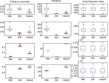
fitting the beta-binomial distribution (d= 2) when all data points have the same batch sizem. Top: m= 5; Middle: m = 10; Bottom: m= 20. 37 Figure 2.7 Comparison of algorithmic timing, convergence rates, and final

objec-tive values under different parameter values. Row 1:α= (0.1,1); Row 2:α= (0.2,2); Row 3: α1 =· · ·=α50 = 0.5; Row 4: α1 =· · ·=α50 =

5. The sample size isn = 200. The batch size ism= 20. There are 100 replicates in each scenario. Convergence criterion is 10−6. . . 39

Figure 3.1 Left: A gene with 3 exons and all possible isoforms. Middle and right: Pairwise scatter plots and correlations of exon counts of a gene with 5 exons. . . 42 Figure 3.2 ROC curves from the group-penalized estimation by the multinomial

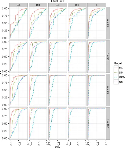
(MN), Dirichlet-multinomial (DM), and generalized Dirichlet-multinomial (GDM) regression models. ROC curves are summarized from 300 simu-lation replicates. Responses are generated from the multinomial (MN) model. . . 102 Figure 3.3 Box plots of AUCs from the group-penalized estimation by the

multino-mial (MN), Dirichlet-multinomultino-mial (DM), generalized Dirichlet-multinomultino-mial (GDM) and negative multinomial (NM) regression models, based on 300 simulation replicates. Responses are generated from the multino-mial (MN) model. . . 103 Figure 3.4 ROC curves from the group-penalized estimation by the multinomial

(14)

Figure 3.5 Box plots of AUCs from the group-penalized estimation by the multino-mial (MN), Dirichlet-multinomultino-mial (DM), generalized Dirichlet-multinomultino-mial (GDM) and negative multinomial (NM) regression models, based on 300 simulation replicates. Responses are generated from the Dirichlet-multinomial (DM) model. . . 106 Figure 3.6 ROC curves from the group penalized estimation by the

multino-mial (MN), multinomultino-mial (DM), and generalized Dirichlet-multinomial (GDM) regression models. ROC curves are summarized from 300 simulation replicates. Responses are generated from the gen-eralized Dirichlet-multinomial (GDM) model. . . 108 Figure 3.7 Box plots of AUCs from the group penalized estimation by the

multino-mial (MN), Dirichlet-multinomultino-mial (DM), generalized Dirichlet-multinomultino-mial (GDM) and negative multinomial (NM) regression models, based on 300 simulation replicates. Responses are generated from the GDM model.109 Figure 3.8 ROC curves from the group-penalized estimation by the multinomial

(MN), Dirichlet-multinomial (DM), and generalized Dirichlet-multinomial (GDM) regression models. ROC curves are summarized from 300 sim-ulation replicates. Responses are generated from the negative multino-mial (NM) model. . . 111 Figure 3.9 Box plots of AUCs from the group-penalized estimation by the

multino-mial (MN), Dirichlet-multinomultino-mial (DM), generalized Dirichlet-multinomultino-mial (GDM) and negative multinomial (NM) regression models, based on 300 simulation replicates. Responses are generated from the negative multinomial (NM) model. . . 112 Figure 3.10 QQ plots of eQTL analysis of ST13P6 using MN, DM, GDM and NM

regressions. ˆλs are the estimated genomic control (GC) inflation factor. 115 Figure 3.11 Manhattan plots of GDM, DM, MN, NM and NegBin regressions for

eQTL analysis of ST13P6. Dashed lines are chromosome-8-wide signif-icance level. . . 116

Figure 4.1 Fitted counts versus the observed counts based on the GDM model. 139 Figure 4.2 Variable selection by the group penalty. Left: BIC trace. Right:

Regu-larized estimate Bb(λ) at the optimal λ displayed in grayscale. . . 141

Figure 4.3 Low rank regression by the nuclear norm penalty. Left: BIC trace. Right: Regularized estimateBb(λ) at the optimalλdisplayed in grayscale.142

Figure 4.4 Select by parameter matrix entries with L1 norm penalty. Left: BIC trace. Right: Regularized estimateBb(λ) at the optimalλ displayed in

(15)

Figure 5.1 Log-likelihood value from fitting Dirichlet-multinomial model with dif-ferent algorithms. The data is generated from i.i.d. DM(1,1,1,1) with sample size 1000. The batch size of each data point is generated from i.i.d. Binomial(80,0.8). . . 173 Figure 5.2 Parameter estimates from fitting Dirichlet-multinomial model with

dif-ferent algorithms. The data is generated from i.i.d. DM(1,1,1,1) with sample size 1000. The batch size of each data point is generated from i.i.d. Binomial(80,0.8). . . 174 Figure 5.3 Case 1: RSS from fitting linear regression with online MM algorithms

and deterministic algorithm. The covariate matrix X is of size n×d,

n = 100, d = 4. Elements of X are generated from i.i.d. N(0,1).

β= 514.Y =Xβ+e, where eis a vector of random error generated

from i.i.d. N(0,1). . . 177 Figure 5.4 Case 1: Parameter estimates from fitting linear regression with online

MM algorithms and deterministic algorithm. The covariate matrix X

is of size n ×d, n = 100, d = 4. Elements of X are generated from i.i.d. N(0,1). β = 514. Y = Xβ+e, where e is a vector of random

error generated from i.i.d. N(0,1). . . 177 Figure 5.5 Case 2: RSS from fitting linear regression with online MM algorithms

n= 100,d= 4.X is generated from a multivariate normal distribution with mean0 and covariance matrixΣ1.β = 514. Y =Xβ+e, where

eis a vector of random error generated from i.i.d. N(0,1). . . 178 Figure 5.6 Case 2: Parameter estimates from fitting linear regression with online

MM algorithms and deterministic algorithm. The covariate matrix X

is of size n ×d, n = 100, d = 4. X is generated from a multivariate normal distribution with mean0 and covariance matrixΣ1. β= 514.

Y =Xβ+e, whereeis a vector of random error generated from i.i.d. N(0,1). . . 178 Figure 5.7 Case 3: RSS from fitting linear regression with online MM algorithms

n= 100, d = 20. X is generated from a multivariate normal distribu-tion with mean 0 and covariance matrix Σ2. β= 5120. Y =Xβ+e,

wheree is a vector of random error generated from i.i.d. N(0,1). . . . 179 Figure 5.8 Case 3: Parameter estimates of β1, β2, β3, β4 from fitting linear

re-gression with online MM algorithms and deterministic algorithm. The covariate matrix X is of size n×d, n = 100, d = 20. X is generated from a multivariate normal distribution with mean 0 and covariance matrix Σ2. β = 5120. Y = Xβ +e, where e is a vector of random

(16)

Figure 5.9 Case 1: RSS from fitting linear regression with online MM, LMS, and RLS. The covariate matrix X is of size n ×d, n = 10000, d = 4. Elements ofX are generated from i.i.d. N(0,1).β = 514.Y =Xβ+e,

wheree is a vector of random error, ei’s are i.i.d. N(0,1). . . 181

Figure 5.10 Case1: Parameter estimates from fitting linear regression with online MM, LMS, and RLS. The covariate matrixX is of sizen×d,n = 10000,

d = 4. Elements of X are generated from i.i.d. N(0,1). β = 514.

Y =Xβ+e, wheree is a vector of random error,ei’s are i.i.d. N(0,1). 181

Figure 5.11 Case 2: RSS from fitting linear regression with with online MM, LMS, and RLS. The covariate matrix X is of size n×d, n = 10000, d= 4.

X is generated from a multivariate normal distribution with mean 0 and covariance matrix Σ1.β = 514. Y =Xβ+e, where e is a vector

of random error, ei’s are i.i.d. N(0,1). . . 182

Figure 5.12 Case 2: Parameter estimates from fitting linear regression with online MM, LMS, and RLS. The covariate matrixX is of sizen×d,n = 10000,

d = 4. X is generated from a multivariate normal distribution with mean 0 and covariance matrix Σ1. β= 514. Y =Xβ+e, where eis

a vector of random error,ei’s are i.i.d. N(0,1). . . 182

Figure 5.13 Case 3: RSS from fitting linear regression with online MM, LMS, and RLS. The covariate matrix X is of size n×d, n = 10000, d = 20. X

is generated from a multivariate normal distribution with mean0 and covariance matrix Σ2. β = 5120. Y =Xβ+e, where e is a vector of

random error, ei’s are i.i.d. N(0,1). . . 183

Figure 5.14 Case 3: Parameter estimates of β1, β2, β3, β4 from fitting linear

re-gression with online MM, LMS, and RLS. The covariate matrix X is of size n×d, n = 10000, d = 20. X is generated from a multivariate normal distribution with mean 0and covariance matrix Σ2. β= 5120.

Y =Xβ+e, wheree is a vector of random error, ei’s are i.i.d. N(0,1).183

Figure 5.15 Log-likelihood value from fitting Dirichlet-multinomial regression with different algorithms. . . 186 Figure 5.16 Parameter estimates ofβ1from fitting Dirichlet-multinomial regression

with different algorithms. . . 187 Figure 5.17 Simulation results of Dirichlet-multinomial distribution parameter

(17)

Chapter 1 Introduction

1.1 Optimization Methods Overview

The central theme of this thesis is about optimization methods. Abundant research has

been done in this area. We first present some of the milestone optimization methods in this

section. Denote the target function as `(θ) whose maximum we seek, where θ∈Θ∈_Rp

is the parameter of interest. To fix notation, differential d`(θ) is the row vector of the partial derivative of `(·) at θ and the gradient ∇`(θ) is the transpose of d`(θ). The Hessian matrix of `(θ) is denoted by d2`(θ).

Newton’s Method

Newton’s method has seen its popularity over years. It is the gold standard for speed

of convergence, and the basis of many variants. Taking second-order Taylor expansion

around the current iterate θ(t) gives

`(θ)≈`(θ(t)) +d`(θ(t))(θ−θ(t)) + 1

2(θ−θ

(t)₎T

(18)

Letd`(θ) = ∂`(θ)/∂θ and ∇`(θ) =d`(θ)T_{. Equating the gradient of the right hand side}

of the equation to0

∇`(θ(t)) +d2`(θ(t))(θ−θ(t)) =0,

we can solve for the next iterate

θ(t+1)=θ(t)−d2`(θ(t))−1∇`(θ(t)).

Although it is easy to derive, Newton’s method has drawbacks. First, the

evalua-tion and inversion of the observed informaevalua-tion matrix −d2_`₍_θ_{) can be computationally}

expensive, especially when the dimensionality of the parameter is high. Second, the

al-gorithm does not guarantee to improve the target function at each iteration such that

`(θ(t+1)₎ _{> `}₍_θ(t)_{). A strict ascending algorithm requires a positive definite observed}

information matrix.

To address these issues, some variants of the Newton’s method are introduced, trying

to approximate −d2_`₍_θ_{) with a positive definite matrix. We put down the general form}

of Newton’s method

θ(t+1) =θ(t)+s[A(t)]−1∇`(θ(t)).

Here,s is a step length used in backtracking strategy, andAis a positive definite matrix. The value of s can be determined in different ways, such as step-halving, where s =

1,1₂, . . ., golden section search, and cubic interpolation.

(19)

Taking A = E[−d2_`₍_θ_{)] gives Fisher’s scoring method. The expected information}

matrix is positive definite, but could be hard to derive or computationally expensive to

evaluate.

Instead of providing an anlytical approximation of A, we can also approximate

−d2_`₍_θ_{) numerically, which leads to the Quasi-Newton method. The approximation of}

−d2_`₍_θ_{) should be positive definite, closest to the previous approximation, and satisfy}

the secant condition

∇`(θ(t−1))− ∇`(θ(t)) =A(θ(t−1)−θ(t)).

Popular Quasi-Newton updates include Davidon-Fletcher-Powell (DFP) rank-2 update.

The updated A(t)=X solves

minimize tr([A(t−1)_]_X−1₎₋_{log det([}_A(t−1)_]_X−1₎

subject to X(θ(t−1)₋_θ(t)_{) =}_∇`₍_θ(t−1)₎_{− ∇`}₍_θ(t)₎

for the next approximation A(t)_{. The update is a low rank update from} _A(t−1)_{. By the}

Woodbury formula (Woodbury, 1950), we can get the updated [A(t)_]−1 _{without directly}

inverting A(t).

Another widely used Quasi-Newton update is the Broyden-Fletcher-Goldfarb-Shanno

(BFGS) rank-2 update (Nocedal and Wright, 2006). BFGS update [A(t)_]−1_{directly, where}

[A(t)_]−1 ₌_X _solves

minimizing tr([A(t−1)_]−1_X₎₋_{log det([}_A(t−1)_]−1_X₎

(20)

Expectation-Maximization (EM) Algorithm

The celebrated expectation-maximization (EM) algorithm (Baum et al., 1970a;

Demp-ster et al., 1977) is one of the most widely used optimization methods in statistics. To

maximize the target log-likelihood`(θ|Y) given the observed dataY, we first construct a complete dataX = (Y,Z) with log-likelihood f(Y,Z|θ). The idea is that the complete data model is easy to optimize, and we can solve for θ iteratively. The iterative two step procedure includes:

E step: compute the conditional expectation of the complete data model

Q(θ|θ(t)) = E_θ(t)[f(Y,Z|θ)|Y =y,θ(t)],

M step: maximizeQ(θ|θ(t)) updateθ(t+1)

θ(t+1) = arg max

θ Q(θ|θ

(t)₎_.

EM algorithm is stable as the ascending property is guaranteed. By information

inequal-ity,

Q(θ|θ(t))−`(y|θ)

= E[f(Y,Z|θ)−`(Y|θ)|Y =y,θ(t)]

≤ E[f(Y,Z|θ(t))−`(Y|θ(t))|Y =y,θ(t)]

(21)

So,

`(y|θ(t+1))≥Q(θ(t+1)|θ(t))−Q(θ(t)|θ(t)) +`(y|θ(t))≥`(y|θ(t)).

EM algorithm depends on constructing complete data models, which limits its usage

to maximizing the log-likelihood functions.

Minorization-Maximization (MM) Principle

In recent years it has been realized that EM algorithm is a special case of the more general

minorization-maximization (MM) principle. The two ‘M’s in MM algorithm stand for

Minorization: find a surrogate functiong(θ) that satisfies

`(θ) ≥ g(θ|θ(t)), for all θ, `(θ(t)) = g(θ(t)|θ(t)).

Maximization: maximize g(θ) and get the updated parameter estimate

θ(t+1) = arg maxg(θ|θ(t)).

The ascent property is guaranteed as

`(θ(t+1))≥g(θ(t+1)|θ(t))≥g(θ(t)) =`(θ(t)).

MM principle possess some advantages over EM algorithm. First, as a general

(22)

functions. Second, by tactfully constructing the surrogate functions, MM algorithm can

save computing power and time. Third, when the dimension of the parameter is high,

MM principle could break it into low dimensional problems, which provides opportunities

to run sub-iterations in parallel.

EM algorithm is a special case of MM algorithm. TheQ(θ|θ(t)_{) function is a particular}

surrogate function. There are cases that both EM and MM algorithms are easy to derive.

The convergence rate is of interest in such cases. In Chapter 2, we perform analysis on a

case study, and investigate the convergence rate of two algorithms. We find that different

algorithms converge at different rate, yet neither algorithm is definitively superior to the

other, and the actual convergence rate is subject to the data set.

The construction of surrogate functions becomes the key in deriving efficient

algo-rithms under MM principle. Manipulating inequalities usually leads to nice surrogate

functions. Let f(·) denote the function we try to maximize. Lange (1999) presented four

ways for constructing minorization functions,

Jensen’s inequality.f(·) is concave, then the minorization is

f(xT

y) =f X

i xiyi

!

≥X

i

xif(yi) =g(x|y).

Linear majorizatoin. f(·) is convex, then the minorization could be

f(x)≥f(y) +df(y)(x−y) =g(x|y).

Minorization with bounded curvature. Iff(·) is twice differentiable, then

f(x)≥f(y) +df(y)(x−y) + 1(x−y)T

(23)

where d2_f₍_x₎₋_B _{is positive definite.}

Arithmetic geometric mean inequality. Foryi >0 andαi >0, and P_iαi = 1,

−Y

i=1

yαi

i ≥ − X

i

αiyi =g(α|y).

Mairal (2013) made another summary of first order surrogate functions when the

target f(·) is possibly non-smooth.

Path Algorithm

We have been discussing maximization problems till now. In the following four small

sections, we abuse the notation `(θ) as the loss function, and target at minimizing it. Several important optimization algorithms emerged motivated by l1 penalized

re-gression. One of the most important is the homotopy algorithm proposed by Osborne

et al. (2000). Let X = (xT

1, . . . ,x

T

n)

T _{denote the covariates, where} _i _{= 1}_{, . . . , n}_, _x

i =

(xi1, . . . , xip)T,Y = (Y1, . . . , Yn)Tdenote the responses, β= (β1, . . . , βp)T denote the

cor-responding regression coefficients. The loss function is `(β) = 1₂||Xβ−Y||2_{, subject to}

Pp

j=1|βj| ≤ λ, where λ > 0 is the constraint parameter. For the current iterate β(t), let

s={j :βj 6= 0}be the index set of nonzero coefficients, and |s|denote the cardinality of

s. Let P present the permutation matrix that collects the nonzero elements of β. Write

β(t)=PT

βs(t)

0

,X =PT

Xs Xsc

.

Let as = sign(βs) have entry 1 if the corresponding entry in βs is positive and −1

otherwise. The homotopy algorithm consists of three steps:

1. optimization. Solve minh`(β(t)+h), subject toaTs(β

(t)

s +hs)≤λ,h=PT h₀s

(24)

solution is

hs = (XsTX)

−1_[_XT

s(y−Xsβs)−µas]

where µ= max

0,a T

s(X

T

sXs)−1XsTy−λ aT

s(XsTXs)−1as

.

2. deletion. Denoteβ†=β(t)₊_h_{. Check sign(}_β†

s) equalsas. We take out the element

ins that violates the equality the most until sign(β_s†) = as.

3. check optimality condition. If the current solution does not satisfies the optimality

condition, we update the set s by adding an element that most violates the

op-timality condition, and return to the optimization step. Otherwise, the algorithm

terminates.

However, Osborne et al. (2000) is trying to solve penalized linear regression. Kim

et al. (2008) point out that the homotopy algorithm may fail to converge when the loss

function is not the squared error loss.

Path-wise Coordinate Descent

Targeting at the l1 regularized regression problem, Wu and Lange (2008) and Friedman

et al. (2007) both propose the “one-at-a-time” coordinate-wise descent algorithm. It

solves a sequences of single-parameter problems. Assuming that the covariate matrix X

is orthogonal for each single parameter, the lasso solution is a soft-thresholded solution

of the least square estimate βLS j ,

(25)

Thus, the high-dimensional optimization problem is reduced top one-dimensional

prob-lems. This solution holds when the covariates are uncorrelated. When the covariates are

correlated, consider

`(β|βk= ˜βk, k6=j) =

1 2

t X

i=1

yi− X k6=j

xikβ˜k−xijβj !2

+λX

k6=j

|β˜j|+λ|βj|.

Minimizing the above function with respect toβj, we get

˜

βj =S t X

1=1

xij(yi−y˜

(j)

i ), λ !

.

Although coordinate descent algorithms enjoy simplicity and computation efficiency, its

convergence requires that `(θ) is convex and differentiable.

Proximal Gradient Method

The goal of proximal gradient method is to optimize convex non-smooth functions. It

requires the target function `(θ) to be split into two terms and at least one of which is differentiable. Denote

`(θ) =f(θ) +h(θ),

where `(θ) is the target function, f(θ) is convex and differentiable, h(θ) is closed, con-vex, and possibly non-differentiable. Martinet (1970) first proposed the idea of proximal

gradient method. The proximal operator of a convex functionh(θ) is

prox_h(θ0) = arg min

θ

h(θ) + 1

2||θ−θ0||

2 2

(26)

An important example is that when h(θ) =λ||θ||1. proxh is the soft thresholding

prox_h(θi) =           

θi−λ θi > λ

0 |θi| ≤λ

θi+λ θi <−λ.

Bruck Jr. (1977) proposed proximal gradient method

θ(t+1) = prox_λ(t)_h(θ(t)−λ(t)∇f(θ(t))),

whereλ(t) _>_{0 is the step size,}_∇f _{is Lipschitz continuous with constant}_L_{, i.e.,}_k∇`₍_θ 1)−

∇`(θ2)k ≤ Lkθ1 −θ2k for all θ1,θ2, and the step size λ(t) ∈(0,L−1). The proximal

gra-dient method is a special case of MM algorithm. Here, the majorizing surrogate function

tof(θ) is

gλf(θ|θ(t)) = f(θ(t)) +df(θ(t))(θ−θ(t)) +

1

2λ||θ−θ

(t)_||2 2.

Given θ(t)_,_g

λf(θ|θ(t)) satisfies majorization property such that

gλf(θ(t)|θ(t)) = f(θ(t))

(27)

1 Initialize θ(0) = (θ₁(0), . . . ,θ_d(0)

e ), and line search parameter a∈(0,1). Let

λ =λ(t−1). repeat

2 Let θ_temp = prox_λf(θ(t)−λ∇f(θ(t))) ; 3 Break if f(θ_temp)≤g_λ(θ_temp|θ(t)) ; 4 Update λ=aλ.

5 until Loss function ` converges; 6 Return λ(t) =λ, θ(t+1) =θtemp.

Algorithm 1: The proximal gradient algorithm provided by Beck and Teboulle (2009a)

The proximal operator is defined as

prox_λh(θ(t)) = arg min

θ

h(θ) + 1

2λ||θ−θ

(t)₊_λ∇f₍_θ(t)₎_||2 2

= arg min

θ

h(θ) +f(θ(t)) +∇f(θ(t))T

(θ−θ(t)) + 1

2λ||θ−θ

(t)_||2 2

= arg min

θ h(θ) +gλf(θ|θ

(t)₎

.

When L is unknown, the step size λ(t) _{can be found by line search. Algorithm 1 is the}

proximal gradient algorithm with line search given by Beck and Teboulle (2009a).

Accelerated Proximal Gradient Method

The proximal gradient method converges at a linear rate O(1/t). Nesterov (1983)

pro-posed an accelerated proximal gradient method that keeps the same computation

com-plexity per iteration, but converges at a quadratic rateO(1/t2_{). It is a simple modification}

of the original proximal gradient method. At each iteration, we get an extrapolation of

(28)

method based on the extrapolated point.

S(t+1) = θ(t+1)+at+1(θ(t+1)−θ(t))

θ(t+1) = prox_λf(S(t+1)−λ∇f(S(t+1)))

whereat∈[0,1) is an extrapolation parameter. Note that the complexity of the

computa-tion is the same as the original proximal gradient method, and only first order informacomputa-tion

is used. Nesterov named it optimal first order method, as the convergence rate is

supe-rior to the original method, and can not be further improved (Nesterov, 1983). Different

versions of the accelerated proximal gradient method are proposed, including Nesterov

(2007); Tseng (2008); Beck and Teboulle (2009b).

1.2 Multivariate Generalized Linear Models

We utilize the above optimization principles to derive algorithms for multivariate

gen-eralized linear models (MGLM). Multivariate count data abound in modern application

areas such as genomics, sports, imaging analysis, and text mining. One of our motivation

is high-throughput data in genomics. Next generation sequencing technology has become

the primary choice for massive quantification of genomic features. The data obtained

from sequencing technologies are often summarized by counts: the number of DNA or

RNA fragments within a genomic interval (Wang et al., 2009; Sun et al., 2014; Trapnell

et al., 2012; Ernst and Kellis, 2012; Hoffman et al., 2012; Zeng et al., 2013).

Multinomial-logit model (McCullagh and Nelder, 1983) becomes a common choice

when analyzing such data, as available software provide handy tools to fit distribution

(29)

mean-variance structure and the implicit assumption that individual counts in the response

vector are negatively correlated. There are multivariate count models that account for

more complex correlation structures. For example the Dirichlet-multinomial model is

good when the counts in the response vector are negatively correlated but have

over-dispersion; the generalized Dirichlet-multinomial model is used when the counts in the

responses have both positive and negative correlations; the negative multinomial model,

which is a multivariate generalization of the negative binomial model can be used to

analyze positively correlated responses. Parameter estimation in these models is typically

hard because they do not belong to the exponential family. Due to the complexity of the

log-likelihood functions, there is no stable algorithm to get parameter estimate for these

models.

In Chapter 3, we develop algorithms that performs distribution fitting, regression, and

variable selection for all four multivariate generalized linear models, namely multinomial

logit (MN), Dirichlet-multinomial (DM), generalized Dirichlet-multinomial (GDM), and

negative multinomial (NM). We propose a unifying iteratively reweighted Poisson

re-gression (IRPR) method for maximum likelihood estimation, which is stable, scalable

to high dimensional data, and extremely simple to implement using existing softwares.

Hypothesis test methods for these models are also studied.

Algorithms for regulated estimates are also developed in Chapter 3. Three penalty

terms are considered: l1, group, and nuclear penalty. Unlike the univariate models where

the regression parameter is a vector, the parameter in multivariate models are matrices.

The three penalty types enable selection by entries, by rows, and by singular values. Both

group penalty and nuclear penalty leads to complex loss functions that MM algorithms

does not work. Another algorithm that is widely used in regularized regression, coordinate

(30)

proximal gradient method (Beck and Teboulle, 2009b) to derive the algorithm.

All the developed algorithms are implemented in the R package MGLM and Matlab

toolboxmglm.

1.3 Online Optimization

The optimization methods we have mentioned so far are all deterministic optimization

methods, where all the data points are available at the same time, and we use the whole

data set to iteratively solve for the optimum. In practice, a huge amount of data could

become available every second. The computation based on deterministic algorithms is

sensitive to the memory limit. How to efficiently perform statistical analysis on the large

cumulative data set becomes a challenging problem; how to update the statistical estimate

with the newly available data is a practical issue. In the last part of this dissertation, we

propose online optimization algorithms that address these issues.

The key idea is to update the parameter estimate based on only a small batch of the

data in each iteration, and the information of the whole data set is used after processing

through each of the small data batches. So, the algorithms is less memory intensive,

because only the small batch of data points are held on the memory in each iteration, and

each data point only gets processed once. The foundation of online algorithms is centered

on stochastic approximation theories. Some widely used deterministic algorithms have

their online analogs. For example, the stochastic gradient algorithms are the analogs of

the deterministic gradient based algorithms (Spall, 2003); Titterington (1984) proposed

an online version of the EM gradient method; Capp´e and Moulines (2009) complemented

the online EM algorithm. The online algorithms share some common properties with

(31)

construction of complete data models; the online gradient based algorithms also suffer

from stability issues. In this dissertation, we propose an online MM algorithm.

1.4 Plan of Dissertation

In Chapter 2, we present a case study comparing the EM and MM principles for the

maximum likelihood estimation of the Dirichlet-multinomial distribution. We also

pro-pose a new EM-MM hybrid algorithm that achieves faster convergence rate in this case.

In Chapter 3, we present the algorithms developed for multivariate generalized linear

models. In Chapter 4, we introduce the software package that implements the algorithms

(32)

Chapter 2 EM vs MM Principles

The celebrated expectation-maximization (EM) algorithm is one of the most widely used

optimization methods in statistics. In recent years it has been realized that EM

algo-rithm is a special case of the more general minorization-maximization (MM) principle.

Both algorithms create a surrogate function in the first (E or M) step that is maximized

in the second M step. This two step process always drives the objective function uphill

and is iterated until the parameters converge. The two algorithms differ in the way the

surrogate function is constructed. The expectation step of the EM algorithm relies on

calculating conditional expectations, while the minorization step of the MM algorithm

builds on crafty use of inequalities. For many problems, EM and MM derivations yield

the same algorithm. This chapter walks through the construction of both algorithms for

estimating the parameters of the Dirichlet-multinomial distribution. This particular case

is of interest because EM and MM derivations lead to two different algorithms with

com-pletely distinct operating characteristics. The EM algorithm converges fast but involves

solving a nontrivial maximization problem in the M step. In contrast the MM updates

(33)

shows faster convergence than the MM algorithm in certain parameter regimes. The local

convergence rates of the three algorithms are studied theoretically from the unifying MM

point of view and also compared on numerical examples.

2.1 Introduction

Numerical optimization methods have been intensively used by statisticians due to the

popularity of the maximum likelihood estimation. A powerful weapon among them is the

expectation-maximization (EM) algorithm (Dempster et al., 1977). The E step in the EM

algorithm creates aQfunction which is then maximized in the M step. In many problems

the surrogateQfunction is much simpler than the log-likelihood and thus the M step can

be solved analytically. These two steps iterate until the parameters converge. In recent

years, it has been realized that the EM algorithm is a special case of the more general

minorization-maximization (MM) principle (de Leeuw, 1994; Heiser, 1995; Lange et al.,

2000; Wu and Lange, 2010). The first M step of an MM algorithm creates a minorizing

function that is optimized in the second M step. TheQfunction in the EM algorithm is a

specific example of minorizing functions. Same as the EM algorithm, this two-step process

always drives the objective function uphill. The key difference between the two algorithms

is the construction of surrogate functions. The minorization step in the MM algorithm

hinges upon recognizing and manipulating inequalities, while EM algorithm relies on

calculating conditional expectations. Advantages enjoyed by both algorithms are their

numerical stability, natural adaption to parameter constraints, and scalability to high

dimensions. An open question has been raised whether any MM algorithm can be recast

as an EM algorithm (Meng, 2000). For instance, the MM algorithms for fitting

(34)

with appropriately chosen latent variables (Caron and Doucet, 2010). However, in these

worked out examples, the construction of missing data framework turns out non-intuitive

and irrelevant to the statistical model that generates the data. Taking the MM point of

view frees the derivation from the dependence on a missing data framework. For instance,

the recent article (Wu and Lange, 2010) demonstrates the potential of the MM algorithm

in random graph models, discriminant analysis, and image restoration problems where

there is no apparent missing data structure.

This chapter walks through the construction of both EM and MM algorithms for

the maximum likelihood estimation of the Dirichlet-multinomial distribution. For this

particular problem they produce two completely different algorithms. TheQ function in

the EM algorithm is fraught with special functions (digamma and trigamma) and the

M step resists analytical solutions and has to resort to iterative, multivariate Newton’s

method. In contrast, the surrogate function of the MM algorithm is much simpler and

yields trivial updates in the M step. Re-inspecting the M step of EM algorithm from

the MM perspective leads to an EM-MM hybrid algorithm which partially resolves the

difficulty in the M step of the EM algorithm. Similar hybrid algorithm is utilized in

fitting mixture of Plackett-Luce models for ranking data (Gromley and Murphy, 2008).

The local convergence rates of the MM and hybrid algorithms are studied theoretically

and demonstrated on numerical experiments. There is no clear winner in the sense that

one converges faster than the others in all parameter regimes.

As a road map to the remainder of this chapter, Section 2.2 lays out the problem

being studied and introduces a classical data set for numerical illustrations. EM and MM

algorithms are derived in Section 2.3 and 2.4 respectively. The difficulty in maximizing

the Q function in the EM algorithm can be partially remedied if we take the MM point

(35)

algorithm. Local convergence properties of the three algorithms are studied in Section

2.6. The operating characteristics (run time, convergence rates, and final objective values)

of the three algorithms are compared numerically under various parameter settings in

Section 2.7. We also provide some other options for solving this problem.

2.2 Problem Setup and a Running Example

Multivariate count data frequently arise in genetics (Lange, 2002; Tvedebrink, 2010;

Ionita-Laza and Laird, 2010), toxicology (Hines and Lawless, 1993), protein

homol-ogy detection (Sj¨olander et al., 1996), word burstiness modeling (Madsen et al., 2005),

and language modeling (MacKay and Bauman Peto, 1994). When multivariate count

data exhibit over-dispersion, the Dirichlet-multinomial distribution is preferred over the

familiar multinomial distribution. In the Dirichlet-multinomial sampling, the

multino-mial parameter p = (p1, . . . , pd) is modeled as a Dirichlet distribution with

parame-ter α = (α1, . . . , αd), where αj > 0. Accordingly, given a multivariate count vector x = (x1, . . . , xd) with batch size m =

Pd

j=1xj, the probability mass function under a

Dirichlet-multinomial model is

f(x|α) =

Z

∆d

m

x d

Y j=1

pxj

j

Γ(|α|)

Qd

j=1Γ(αj)

d Y j=1

pαj−1

j dp (2.1)

=

m

x Qd

j=1Γ(αj +xj)

Γ(|α|+m)

Γ(|α|)

Qd

j=1Γ(αj)

=

m

x Qd

j=1(αj)xj

|α|m

(36)

where|α|=Pd_j₌₁αj and (a)k=Qk

−1

i=0(a+i) denotes the rising factorial. The last equality

is due to the fact Γ(a+k)/Γ(a) = (a)k. An alternative parametrization uses

πj =

αj

|α|, j = 1, . . . , d, θ=

1

|α|, (2.3)

in terms of the proportion vector π = (π1, . . . , πd) and the over-dispersion parameter θ.

For the sake of brevity, we stick to parametrization (2.2) in this article. The derivation

and most conclusions equally apply to both parameterizations. Given independent data

points x1, . . . ,xn, the log-likelihood is

`(α) =

n X

i=1

lnf(xi|α)

=

n X

i=1

ln

mi xi

+

n X

i=1

d X

j=1

xij−1

X k=0

ln(αj+k)− n X

i=1

mi−1

X k=0

ln(|α|+k) (2.4)

and the maximum likelihood estimation seeks the maximizer of (2.4). Most current

ap-plications utilize the Newton’s method for finding the MLE (Lange, 2002; Tvedebrink,

2010; Ionita-Laza and Laird, 2010), which may be numerically instable because the

objec-tive function (2.4) is non-concave. The alternaobjec-tive Fisher’s scoring algorithm replaces the

observed information matrix in Newton’s method by expected information matrix and

yields an ascent algorithm. However, the calculation of expected information matrix for

Dirichlet-multinomial model is expensive due to numerous evaluations of beta-binomial

tail probabilities (Paul et al., 2005). Recently Zhou and Lange (2010) devise the MM

algo-rithm for a whole class of multivariate discrete distributions which include the

Dirichlet-multinomial as a special case. Compared to the Newton’s method, the MM algorithm is

(37)

take up the alternative EM approach for maximizing the log-likelihood (2.4) and contrast

it to the MM algorithm in respect to algorithmic design, per iteration computation cost,

and local convergence rate.

As a numerical example we consider the classical data on the mice that are exposed to

various mutagens (Haseman and Soares, 1976). Environmental scientists are interested

in investigating the mutagenicity of a compound or irradiation in vivo in mice. Male

mice are treated with the suspect mutagen and then paired to one or more female mice.

Seventeen days after the initial exposure to a male, females are killed and their uteri are

examined for the presence of living and dead embryos (implants). In the first data set of

Haseman and Soares (1976), denoted by HS76-1 in following, there are n= 524 females

with the total number of implants per female mi varying from 1 to 20. Counts of dead

and survived implants are recorded for each female. Figure 2.1 displays the histogram

of the 524 proportions of dead implants. The variability in the proportions is prominent

and the traditional binomial distribution is inappropriate for such over-dispersion count

data. Fitting the beta-binomial distribution (d = 2) to the HS76-1 data set gives the

MLE ˆα= (1.23,12.46) with log-likelihood −777.79. The density of the beta distribution with parameter ˆα is imposed on the histogram in Figure 2.1 and demonstrates a good fit. The classical binomial fit gives a log-likelihood −842.61. The likelihood ratio test of

the over-dispersion parameter H0 : θ = (α1+α2)−1 = 0 vs H1 : θ > 0 yields a p-value

essentially 0, corroborating the appropriateness of a beta-binomial model.

The performances of the EM, MM and a hybrid algorithm on this data set will be

compared in Section 2.6. Note although we use a d= 2 data set as the running example

for ease of illustration and visualization, all our derivations and convergence rate results

are for generald and numerical experiments are carried out fordas high as 50 in Section

(38)

0 0.2 0.4 0.6 0.8 1 0

0.05 0.1 0.15 0.2 0.25 0.3 0.35 0.4 0.45

proportion of dead implants

frequency

Figure 2.1: Histogram of the 524 proportions in the Haseman and Soares data with a Beta(1.23,12.46) density imposed.

2.3 EM Algorithm

Derivation of EM algorithm hinges upon a missing data structure. Let f(θ) be the log-likelihood of the observed data with parameter vector θ. In the E step, a surrogate function Q(θ|θ(t)_{) is calculated as the conditional expectation of the complete data}

log-likelihood given current parameter iterateθ(t)_{. The well-known calculations (Baum et al.,}

1970b; Dempster et al., 1977) demonstrate that theQfunction satisfies the fundamental

inequality

f(θ)−f(θ(t))≥Q(θ|θ(t))−Q(θ(t)|θ(t)). (2.5)

Maximizing the surrogate Q(θ|θ(t)_{) with respect to} _θ _{generates the next iterate} _θ(t+1)

which obviously drives the log-likelihood of the observed data uphill.

The admixture representation (2.1) of the Dirichlet-multinomial distribution naturally

(39)

the joint density of complete data by Qn_i₌₁f(xi,pi,α). Then the Qfunction is

Q(α|α(t)) = E " _n

X i=1

f(xi,pi,α)|x1, . . . ,xn,α(t) #

,

where the expectation is with respect to the conditional distribution

f(p1, . . . ,pn|x1, . . . ,xn,α(t)),

i.e., independent Dirichlet(xi+α(t)). Therefore

Q(α|α(t)) =

n X

i=1

Qi(α|α(t))

with

Qi(α|α(t))

= Z

∆d

Γ(mi+|α(t)|)

Qd

j=1Γ(xij+α(jt))

Y

j

pxij+α

(t)

j −1

ij

·



ln

mi

xi

+

d

X

j=1

(xij+αj−1) lnpij+ ln Γ(|α|)−

d

X

j=1

ln Γ(αj)



dpi

= ln

mi

xi

+

d

X

j=1

(xij+αj−1)

h

Ψ(xij +α(jt))−Ψ(mi+|α(t)|)

i

+ ln Γ(|α|)−

d

X

j=1

ln Γ(αj).

Here Ψ(z) = Γ0(z)/Γ(z) is the digamma function and the exponential family

(40)

Therefore

Q(α|α(t)) =

n

X

i=1 ln

mi

xi

+

n

X

i=1

d

X

j=1

(xij +αj −1)

h

i

+nln Γ(|α|)−n

d

X

j=1

ln Γ(αj)

=

d

X

j=1

n

X

i=1

αj

h

Ψ(xij+α(jt))−Ψ(mi+|α(t)|)

i

−n

d

X

j=1

ln Γ(αj)

+nln Γ(|α|) +c(t). (2.6)

We use c(t) _{to collect constants that are irrelevant to the optimization and it may vary}

in different equations. MaximizingQ(α|α(t)) is not trivial sinceαj are intertwined in the

ln Γ(|α|) term. The Newton’s method has to be utilized for the M step. The first two derivatives ofQ(α|α(t)_{) are}

[∇Q(α|α(t))]j =

∂Q ∂αj

=X

i

[Ψ(xij +α

(t)

j )−Ψ(mi+|α(t)|)] +nΨ(|α|)−nΨ(αj)

[d2Q(α|α(t))]jj0 = ∂

2_Q

∂αjαj0 =nψ(

|α|)−nψ(αj)1{j=j0_},

where ψ(z) = Ψ0(z) is the trigamma function. Newton’s method iterates according to

α(m+1) =α(m)−[d2Q(α(m)|α(t))]−1· ∇Q(α(m)|α(t)),

where the subscript m indicates its iteration number. Several issues arise here. First, in

each iteration the Hessian matrix d2_Q₍_α_|_α(t)_{) has to be computed and a linear system}

needs to be solved. Second, since the Q function is non-concave (note ln Γ is convex),

the Newton’s method may not generate an ascent algorithm. Even when its Hessian is

(41)

Lastly the Newton’s updates may violate the parameter constraints αj > 0. At this

point it is realized that the EM principle has not reduced the difficulty of the original

optimization problem and the Newton’s or Fisher’s scoring method could be used directly

on the observed data log-likelihood (2.4). However there is a remedy. Before that we first

explore the MM solution.

2.4 MM Algorithm

Like EM, the MM algorithm is a general principle for creating optimization algorithms.

The survey papers (Lange et al., 2000; Hunter and Lange, 2004) and textbook treatment

(Lange, 2010) serve as an excellent introduction. The derivation in this section also

appears in (Zhou and Lange, 2010) as a special case. Letf(θ) be the objective function, not necessarily a log-likelihood, whose maximum we seek. An MM algorithm involves

minorizing f(θ) at current iterate θ(t) _{by a surrogate function} _g₍_θ _| _θ(t)_{) that satisfies}

two properties

f(θ) ≥ g(θ|θ(t)), θ 6=θ(t) (2.7)

f(θ(t)) = g(θ(t) |θ(t)). (2.8)

In other words, the surfaceθ7→g(θ |θ(t)) lies below the surfaceθ 7→f(θ) and is tangent to it at the current iteration θ = θ(t)_{. The construction of the minorizing function}

g(θ | θ(t)_{) constitutes the first M of the MM algorithm. The second M of the MM}

algorithm maximizes the surrogate g(θ|θ(t)_{) rather than} _f₍_θ_{) directly. If} _θ(t+1) _denotes

(42)

It follows directly from the inequalities

f(θ(t+1)) ≥ g(θ(t+1) |θ(t)) ≥ g(θ(t) |θ(t)) = f(θ(t)).

This ascent property is the source of the MM algorithm’s numerical stability and remains

valid if we merely increase g(θ|θ(t)_{) rather than maximize it.}

The fundamental inequality (2.5) in the EM algorithm shows that the Q function

produced in the E step constitutes a minorizing function of the log-likelihood up to an

additive constant. This fact readily qualifies EM algorithm as a special case of the MM

algorithm. The MM perspective is more general as it frees algorithm derivation from

the missing data straitjacket and invites wider applications. Wu and Lange (2010) briefly

summarize the history of the MM algorithm and showcase its flexibility in some problems

in which the EM derivation is hard to carry out.

To construct an MM algorithm for maximizing the Dirichlet-multinomial log-likelihood

function (2.4), the strategy is to minorize term by term. We first simplify the two sums

n X

i=1

d X

j=1

xij−1

X k=0

ln(αj+k) = n X

i=1

d X

j=1

maxixij−1

X k=0

ln(αj +k)1{xij−1≥k}

=

d X

j=1

maxixij−1

X k=0

ln(αj +k) n X

i=1

1{k≤xij−1} =

d X

j=1

maxixij−1

X k=0

sjkln(αj+k)

and

−

n

X

i=1

mi−1 X

k=0

ln(|α|+k) =−

mi−1 X

k=0

ln(|α|+k)

n

X

i=1

1{k≤mi−1}

=−

maximi−1 X

k=0

(43)

where

sjk = n X

i=1

1{xij≥k+1}, rk =

n X

i=1

1mi≥k+1

are counts. Applying the Jensen’s inequality to the ln(αj +k) terms

ln(αj+k)≥

α(_jt) α(_jt)+k

ln α

(t)

j +k

α(_jt) ·αj

!

+ k

α(_jt)+k

ln α

(t)

j +k

k ·k

!

= α

(t)

j

α(_jt)+k

lnαj+c(t) (2.9)

and the supporting hyperplane inequality to the −ln(|α|+k) terms

−ln(|α|+k)≥ −|α| − |α

(t)_|

|α(t)_|₊_k −ln(|α

(t)_|₊_k₎

=− |α|

|α(t)_|₊_k+c

(t) _(2.10)

yields the surrogate function

g(α|α(t)) = −X

k

rk

|α(t)_|₊_k|α|+

X j

X k

sjkα

(t)

j

α(_jt)+k

lnαj +c(t).

Figure 2.2 depicts the two minorization inequalities (2.9) and (2.10) withα(t)_{= 2 and}_k₌

1. In both minorizations, the equality holds at α=α(t). Finding theα that maximizes

g(α|α(t)) is trivial and leads to the multiplicative MM updates

α(_jt+1)=α(_jt)

P k

sjk

α(_jt)+k P

k rk |α(t)_|₊_k

, j = 1, . . . , d, (2.11)

(44)

0 1 2 3 4 5 −1

−0.5 0 0.5 1 1.5 2

f(α(t) )=g(α(t)

|α(t) )=ln(3)

α

f(α)=ln(α+1) g(α|α(t)),α(t)=2

0 1 2 3 4 5

−2.5 −2 −1.5 −1 −0.5 0

f(α(t))=g(α(t)|α(t))=−ln(3)

α

f(α)=−ln(α+1) g(α|α(t)),α(t)=2

Figure 2.2: Graphs of minorization inequalities (2.9) and (2.10).

parameter constraints αj > 0 are always satisfied whenever α

(0)

j > 0. Besides offering a

completely different algorithm from EM, MM principle also suggests a remedy for the

troublesome M step in the EM algorithm.

2.5 An EM-MM Hybrid Algorithm

Due to the fact that the ln Γ(x) function is convex, we can resort to the supporting

hyperplane inequality to separate the parameters in the ln Γ(|α|) term in the Qfunction (2.6)

Q(α|α(t))

≥ X

i

ln

mi

xi

+X

i

X

j

(xij+αj−1)

h

i

+nΨ(|α(t)|)(|α| − |α(t)|) +nln Γ(|α(t)|)−nX

j

ln Γ(αj) +c(t)

= X

j

(

αj

X

i

h

Ψ(xij+α(_jt))−Ψ(mi+|α(t)|) + Ψ(|α(t)|)

i

−nln Γ(αj)

)

(45)

In this new minorizing function (2.12), the parameters αj are separated and only need

to be optimized independently. Equating the partial derivatives with respect to αj to 0

gives the function to solve for αj

X i

Ψ(xij +α

(t)

j )−nΨ(αj) = X

i

Ψ(mi+|α(t)|)−nΨ(|α(t)|).

In view of the recurrence relation Ψ(y+ 1) = Ψ(y) + 1/y, this is equivalent to

Ψ(α(_jt))−Ψ(αj) =

1

n

n X

i=1

mi−1

X k=0

1

|α(t)_|₊_k −

1

n

n X

i=1

xij−1

X k=0

1

α_j(t)+k

= 1

n

maximi−1

X k=0

rk

|α(t)_|₊_k −

1

n

maxixij−1

X k=0

sjk

α(_jt)+k .

It is interesting to note that the two sums on the right hand side were used in the MM

updates (2.11) in a completely different way. Here we can find the root of Ψ(αj) =a by

Newton’s iterates

α(m+1) =α(m)−

Ψ(α(m))−a

ψ(α(m))

.

Since ln Γ is convex, the trigamma function ψ is positive and the Newton’s method is

guaranteed to converge to the right root. The Newton’s method applied to individual

αj is substantially simpler than the multivariate Newton’s method in the original EM

algorithm, which involves computing and inverting Hessian matrix in each iteration. As

(46)

0 50 100 150 −880

−870 −860 −850 −840 −830 −820 −810 −800 −790 −780 −770

Iteration

logL

EM Hybrid MM

0 50 100 150

−880 −870 −860 −850 −840 −830 −820 −810 −800 −790 −780 −770

Iteration

logL

EM Hybrid MM

Figure 2.3: Algorithmic iterates for the HS76-1 data set. Left: Start from a blind guess

α(0) _{= (1}_,_{1). Right: Start from the method of moment estimate} _α(0) _{= (0}_.₄₇₁₁_,₄_._8072).

2.6 Convergence Rates

The EM, MM, and hybrid algorithms constructed so far enjoy the same ascent property,

yet with distinct per iteration computational cost. A formal comparison entails a close

study of their local convergence rates, which roughly measure how fast they converge near

the optimal point. Figure 2.3 displays the iterates of the three algorithms for the HS76-1

data set with two different starting points. When starting from a blind guessα(0) _{= (1}_,_1),

the EM algorithm converges quickly within 20 iterations, while the other two lag behind.

The hybrid algorithm outruns MM initially but is caught up when close to the optimal

point. When starting from the method of moment estimate α(0) = (0.4711,4.8072), EM behaves similarly while the MM algorithm narrowly edges out the hybrid algorithm.

Because all three algorithms can be deemed as special cases of the MM principle, their

convergence properties can be studied under a unified framework. Consider an MM map

(47)

When close to the optimal point θ∞,

θ(t+1)−θ∞≈dM(θ∞)·(θ(t)−θ∞),

where dM(θ∞) is the differential of the mapping M at the optimal point θ∞ of f(θ). Figure 2.4 displays the distance of the algorithmic iterates to the MLE for the HS76-1

example on the logarithmic scale and shows the linear convergence behavior when close

to θ∞. Therefore the local convergence rate of the sequence θ(t+1) ₌_M₍_θ(t)_{) is defined}

as the spectral radius of dM(θ∞). The familiar calculations (McLachlan and Krishnan, 2008; Lange, 2010) demonstrate that

dM(θ∞) = I−[d2g(θ∞|θ∞)]−1d2f(θ∞). (2.13)

In other words, the local convergence rate is determined by how well the surrogate

func-tion g approximates the log-likelihood surface f near the optimal pointθ∞. In EM liter-ature, dM(θ∞) is called the rate matrix (Meng and Rubin, 1991). A smaller rate means that the surrogate functiong(θ|θ∞) hugsf(θ) tighter aroundθ∞and thus implies faster convergence.

In our case, the Q function of the EM algorithm by construction dominates the

minorizing function (2.12) of the hybrid algorithm. This implies the faster convergence of

the EM algorithm than the hybrid algorithm as observed in Figure 2.3. However, there is

no dominance relations between them and the MM surrogate function. Figure 2.5 displays

the log-likelihood surface of the HS76-1 data set and the minorizing functions of the three

algorithms at the parameter point (α1, α2) = (0.5,5). All three minorizing functions lie

(48)

0 100 200 300 400 500 10−5

10−4 10−3 10−2 10−1 100 101

Iteration

||

θ

(t)−

θ

*||

EM Hybrid MM

Figure 2.4: Distance of algorithmic iterates to the final solution kθ(t) −θ∞k2 for the

HS76-1 data set.

of the EM algorithm approximates the log-likelihood function better than the minorizing

function of the hybrid algorithm over the whole region. The MM minorizing function

intersects with the other two besides the point (0.5,5).

Given a data set, the local convergence rates of the three algorithms can be calculated.

Letα∞ be the MLE and define constants

a =

maximi−1

X k=0

rk

(|α∞_|₊_k₎2

bj =

maxixij−1

X k=0

sjk

(α∞_j +k)2, j = 1, . . . , d

cj =

maxixij−1

X k=0

sjk

α∞_j (α_j∞+k), j = 1, . . . , d

dj =nψ(α∞j ) =

∞

X k=0

n

(α_j∞+k)2, j = 1, . . . , d

e =n−1[ψ(|α∞|)−1−X

j

(49)

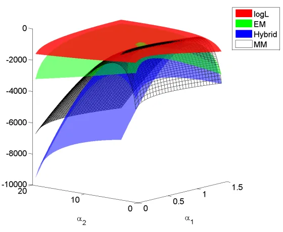
Figure 2.5: Log-likelihood surface and the minorizing functions of EM, MM, and the EM-MM hybrid algorithms at point (0.5,5) for the HS76-1 data set.

and three polynomials

PMM(λ) =

d Y j=1

(λ−bjc−j1) +a d X

j=1

c−_j1 Y

j0₆₌_j

(λ−bj0c−1

j0 )

Phybrid(λ) =

d Y j=1

(λ−bjd−j1) +a d X

j=1

d−_j1Y

j0₆₌_j

(λ−bj0d−1

j0 ) (2.14)

PEM(λ) =

d Y j=1

(λ−bjd−j1)− X

j

(bjd−j1e−ae X

j00

d−_j001−a)d

−1

j Y j0₆₌_j

(λ−bj0d−1

j0 ).

All roots of these polynomials are real and especially the smallest roots give the

informa-tion about the local convergence rates of the algorithms. Formally we have the following

result.

Selected Topics in Statistical Computing.

ABSTRACT

DEDICATION

BIOGRAPHY

ACKNOWLEDGEMENTS

TABLE OF CONTENTS

LIST OF TABLES

LIST OF FIGURES

Chapter 1

Introduction

1.1

Optimization Methods Overview

1.2

Multivariate Generalized Linear Models

1.3

Online Optimization

1.4

Plan of Dissertation

Chapter 2

EM vs MM Principles

2.1

Introduction

2.2

Problem Setup and a Running Example

2.3

EM Algorithm

2.4

MM Algorithm

2.5

An EM-MM Hybrid Algorithm

2.6

Convergence Rates