Copyright1998 by the Genetics Society of America
On the Sampling Variance of Intraclass Correlations and Genetic Correlations
Peter M. Visscher
University of Edinburgh, Institute of Ecology and Resource Management, Edinburgh EH9 3JG, Scotland Manuscript received February 3, 1997
Accepted for publication March 23, 1998
ABSTRACT
Widely used standard expressions for the sampling variance of intraclass correlations and genetic correlation coefficients were reviewed for small and large sample sizes. For the sampling variance of the intraclass correlation, it was shown by simulation that the commonly used expression, derived using a first-order Taylor series performs better than alternative expressions found in the literature, when the between-sire degrees of freedom were small. The expressions for the sampling variance of the genetic correlation are significantly biased for small sample sizes, in particular when the population values, or their estimates, are close to zero. It was shown, both analytically and by simulation, that this is because the estimate of the sampling variance becomes very large in these cases due to very small values of the denominator of the expressions. It was concluded, therefore, that for small samples, estimates of the heritabilities and genetic correlations should not be used in the expressions for the sampling variance of the genetic correlation. It was shown analytically that in cases where the population values of the heritabili-ties are known, using the estimated heritabiliheritabili-ties rather than their true values to estimate the genetic correlation results in a lower sampling variance for the genetic correlation. Therefore, for large samples, estimates of heritabilities, and not their true values, should be used.
T
HERE are three classic papers on the topic of sam- tions for beef cattle traits, argued that using the esti-pling variances of estimates of genetic correlations mates of heritabilities and genetic correlations in the in the 1950s: Reeve (1955), who derived expressions expressions ofReeve(1955) andRobertson (1959a),of the sampling variance for parent-offspring designs; rather than their true (population) values, appeared to
Robertson (1959a), who derived general expressions be closer to the observed empirical sampling variance
for balanced one-way ANOVA designs with equal popu- of the genetic correlation coefficient. This was corrobo-lation values for heritabilities; andTallis(1959), who rated by a small simulation study. Furthermore, these
derived general expressions for balanced and unbal- authors implied that the equations derived in Reeve
anced one-way designs. Although the latter article is, in (1955) and Robertson (1959a) were inaccurate,
be-a sense, the most generbe-al, it is not referred to frequently cause the empirical sampling variance of estimated ge-(it does not help that the reference added in the proof netic correlation coefficients was much larger than the of theRobertsonarticle points to the wrong journal). expected sampling variance, using both their data and
It could be argued that the expressions derived in simulations.
those articles are no longer relevant, since estimation Three areas of confusion can be identified: techniques have moved on from least-squares methods
1. Should the parameters in the expressions for the to likelihood-based methods [mainly r esidual maximum
sampling variance of the genetic correlation
coef-likelihood (REML);PattersonandThompson(1971)].
ficient inReeve(1955),Robertson(1959a), and
Using likelihood methods, sampling variances can be
Tallis (1959) be the population parameters or
approximated from likelihood profiles (Meyer and
the estimates of those parameters?
Hill 1991). However, numerous publications,
particu-2. How good are the expressions derived in the trio larly in the evolutionary genetics literature, still use the
of articles? expressions derived byReeve, Robertson, andTallis.
There appears to be some confusion about the use of 3. What is the impact of estimates that are outside expressions for the sampling variance of genetic correla- the parameter space, i.e., negative heritability esti-tions. For example, Koots and Gibson (1996), who mates and/or estimates of genetic correlations
performed a meta-analysis of an impressive number ,21 or.11? (1500) of estimates of heritabilities and genetic
correla-In this article I review the main expressions ofReeve,
Robertson, andTallisand clarify under what
circum-stances the expressions should be used. I also review Address for correspondence: University of Edinburgh, Institute of
Ecol-and evaluate the equations for the sampling variance
ogy and Resource Management, West Mains Rd., Edinburgh EH9
3JG, Scotland. E-mail: [email protected] of intraclass correlations as a paradigm, since these are
RobertsonandLerner(1949) quoted Fisher, but used
central to the understanding of the assumptions and
methods. c
251/[(s22)n (n21)] . (5)
Finally, followingZerbeandGoldgar(1980), an expression can be derived using
MATERIALS AND METHODS
y5B/W5[11(n21)tˆ]/[12tˆ ] To answer the above questions, we first look at the derivation
of the sampling variance of intraclass correlation coefficients z{[12t]/[11(n21)t]} Fs
21, s(n21).
because this serves as an appropriate paradigm for the
sam-pling variance of the genetic correlation coefficient. Subse- Hence, quently, expressions for the sampling variance of the genetic
var(tˆ)≈[d tˆ/dy]2var(y)5f (t) c 3
correlation are reviewed and evaluated.
with Sampling variance of intraclass correlation coefficients
c35[s(n21)]2[sn23]/[n2(s21)
Population parameters known:Consider a simple, balanced
(s (n21)22)2(s (n21)24)] . (6)
one-way design with s sires and n progeny per sire, and assume
that parameters are estimated using least-squares methods, Although this expression is trivial to derive, to my knowledge e.g., ANOVA. Observations are assumed to be normally distrib- this is the first time that it has been documented following a uted. The expectations and variances of the between- and first-order approximation using the F ratio.
within-sire mean squares (MS) are All the above expressions for ci reduce to the one most commonly used (i.e., c051/[n(s21)(n 21)]) for large s
E[B ]5[(12t)1nt]s2 p,
and n. However, even for large n, there are discrepancies E[W ]5[(12t)]s2
p, between the formulas depending on the use of s, (s21), or
(s22) in the denominator. It is likely that the form used by var(B)52{[(12t)1nt]s2
p}2/[s21] , RobertsonandLerneris incorrect and probably stems from
the use ofFisher’s z-transformation.Fishershowed that var(W )52{[(12t)]s2
p}2/[s(n21)] .
var(z)≈n/[2(n21)(s22)] , with B and W the between- and within-sire MS, t the
popula-tion intraclass correlapopula-tion, andsp the phenotypic standard
with deviation. The variance of the least-squares estimate of the
intra-class correlation, z51⁄
2log{[11(n21)tˆ]/[12tˆ]}.
tˆ5[(B2W )/n]/[(B2W )/n1W ]
Hence,
5[B2W ]/[B1(n21)W ]5A/C ,
var(tˆ )≈[dtˆ/dz]2var(z)5{4(12t)2[11(n21)t]2/n2]}
can be approximated using a first-order Taylor-series
expan-{n/[2(n21)(s22)]} sion about the expected mean squares,
5f (t)c2.
var(tˆ)≈var(A)/E2(C )1E2(A)var(C )/E4(C )
However, as pointed out byOsborneandPaterson(1952),
22E(A)cov(A,C )/E3(C )
this is a roundabout way of deriving the sampling variance of
52(12t)2[11(n21)t]2[(sn21)/
the estimated intraclass correlation, by first transforming to z and then back again.
(n2s(s21)(n21))]
Population values unknown:Except when doing power cal-culations and/or investigating the design of experiments
≈2(12t)2[11(n21)t]2/[(s21)n (n21)] . (1)
(Robertson1959b) or simulation studies, we do not know Equation 1 is well known (Robertson1959b;Falconerand
the population values and hence do not know the exact or Mackay1996). Its derivation, using means and variances of
approximate sampling variance of the intraclass correlation. mean squares, appears to be first given byOsborneand
Pat-The standard practice is to use the formulae derived in the erson(1952).
previous section and to substitute tˆ for t. This is essentially For large n, Equation 1 reduces to based upon the assumption that E (tˆ)5t. However, it should be obvious that if, by chance, the estimate of the intraclass var(tˆ)≈2t2(12t)2/(s21) . (2)
correlation is too high (or too low), the resulting estimate of A number of expressions similar to Equation 1, which all the sampling variance will be biased. Using
differ in the terms relating to the number of sires and progeny
d{f (t)}/dt54[12t][11(n21)t] per sire, can be found in the literature. They differ in
particu-lar in the degrees of freedom relating to the between-sire [(n21)(122t)21] (7) component of variance. The general expression is
gives a maximum estimate of the sampling variance of tˆ 5
var(tˆ)≈f (t) ci (3) 1/
2[(n22)/(n21)] (see alsoTaylor1976). The minimum
estimate of the sampling variance is found for tˆ 51 or tˆ5 with
21/(n21). Only when there is a scale on which the sampling f (t)52(12t)2[11(n21)t]2,
variance is (nearly) independent of the population values, for example, Fisher’s z-scale, will the estimate of the sampling Where ciis a function of s and n, from reference i . The original
variance be correct. expression was derived in a classical paper byFisher(1921),
pling variance of an estimate of the intraclass correlation, This is the scenario ofRobertson(1959a). The terms P and Q simplify to
since
var(MS)52E2(MS)/d.f., P (t
15t2)5(1/R2)[(11r2g)(11{rgR1rw(12R)}2)
24rg(rgR1rw(12R))] , (12)
E [2MS2/(d.f.12)]52[var(MS)1E2(MS)]/(d.f. 12)
52[E2(MS){2/d.f.11})/(d.f.12) Q(t
15t2)5[(12R]/R]2[(11r2g)(11r2w)24rgrw] (13)
52 E2(MS)/d.f.5var(MS) , with
where d.f. is degrees of freedom. This indicates an unbiased R5n/(n1(12t)/t) . estimate of the sampling variance as
These correspond to the equations given by Robertson (1959a, p. 473), although his P and Q were scaled by a factor vaˆr(tˆ)≈2(12tˆ)2(11(n21)tˆ )2 (sn23)
n2(s11)(s (n21)12) of (nt)2.
2. t15t25t and rg5rw5r .
5f (tˆ)c4. (8)
A further simplification is if the genetic and within-sire correla-Equation 8 reduces to the standard equation ofOsborneand
tion are the same. The expression for the sampling variance Paterson(1952) andRobertson(1959b) for large sn.
may be written as Simulation study:Simulations were performed to compare
the empirical standard deviation of heritability estimates, the var(rˆ
g)≈[(12r2)2/R2] [1/(s21)
predicted standard deviation using the true population values
1(12R)2/(s (n21))], (14)
(Equation 1), and the average estimated standard deviation (using Equations 1, 4, and 8, with tˆ substituted for t).
Indepen-which corresponds toRobertson’s formula on page 474. In dent between-sire and within-sire sums of squares were
sam-general, when t1≠t2, there is no simple form for the sampling
pled from centralx2distributions with (s21) and [s (n21)]
variance of the genetic correlation coefficient. degrees of freedom, respectively, and then scaled to the
appro-Finally, Robertson (1959a) suggested a very simple and priate mean squares using the population values of t andsp
general expression for the sampling variance of the genetic and the values of s and n. Without loss of generality, a
pheno-correlation coefficient by observing the similarity between ex-typic standard deviation of unity was used throughout.
pressions derived for special cases, Since the only difference between the various prediction
equations for the sampling variances are functions of s and var(rˆg)≈(12r2
g)2[var(hˆ21)var(hˆ22)]1/2 /[2h21h22] . (15)
n, only results for the Taylor series (OsborneandPaterson
This was the equation used byKootsandGibson(1996). 1952) are presented. The other equations for the sampling
vari-ance differ approximately by factors of (s21)/s (usingFisher’s
3. n→∞, i.e., Ri51. formula) and (s21)/(s11) (usingKempthorne1957).
For a large number of progeny per sire, Tallis’ equation reduces to a very simple form,
Sampling variance of genetic correlation coefficient
var(rˆg)≈(12r2g)2/(s21) . (16)
Expressions from literature:Tallis(1959) derived a
gen-This equation is equivalent to the approximation of the sam-eral expression for the approximate sampling variance of the
pling variance of a correlation coefficient in the bivariate estimated genetic correlation coefficient for a balanced
half-normal case with (s21) degrees of freedom. sib design. Population values for the intraclass correlations of
There are difficulties in using the approaches for the sam-the two traits are t1 and t2, and the genetic and within-sire
pling variance of the intraclass correlation to determine the correlation coefficients are rgand rw, respectively. The general
sampling variance of estimates of the genetic correlation coef-form ofTallis’ expression is
ficient: (1) The estimate of rgis unbounded in principle, so
var(rˆg)≈P /(s21)1Q/(s(n21)) , that large positive and negative values (outside the range21 to
11) are possible, and (2) the true heritability, or its estimate, for
appears in both the numerator and the denominator of the equation for the sampling variance of rg(see Equations 9 to
P5(11r2
g)[1/(R1R2)1A2]22rg(1/R111/R2)A
11). This means that in the vicinity of true or estimated h2
1r2
g(t12t2)2/[2(nt1t2)2] (9) being zero, the estimate of the sampling variance can become
very large because of a division by a small number. Also, if and
one or both of the estimated heritabilities is,0, the estimate Q5(1/R121)(1/R221)[(11r2g)(11rw2) of the genetic correlation coefficient is an imaginary number
(Reeve1955). Simulation results are less meaningful in these
22rg(A2rg)]1r2g(t12t2)2/[2(nt1t2)2] (10)
cases, because the estimate of the sampling variance may not have converged (or never will). For example, in the simulation with
study of parent-offspring regression in Koots and Gibson A5rg1rw[(1/R121)(1/R221)]1/2. (11) (1996), with true population parameters of h2
1 5h22 5 0.10
and rg50, the estimates of rgvaried from22.5 and14.18,
Ri5n/(n1(12ti)/ti), which is the general expression of
and the empirical variance of estimated genetic correlation the reliability of a progeny test based upon n progeny and a
coefficients was very large when both estimates of the heritabil-heritability of 4ti.Tallis(1959) used a different (but
equiva-ity were close to zero. lent) expression for P and Q, but we find it more convenient
Heritabilities known:KootsandGibson(1996) argued that to write the terms as presented here.
in some (rare) cases, the population heritabilities may be Special cases:
ture values. In that case, one could proceed with only estimat- products were used to calculate least-squares estimates of the two heritabilities and the genetic and within-sire correlation ing the between- and within-sire covariances, along with the
phenotypic variances, from the data. If the phenotypic vari- coefficients in the standard way (see, for example, Tallis 1959). For estimated sire variances that were positive, estimates ances are assumed to be estimated accurately, i.e., for large
sn, then of genetic correlations could be,21 or.1. A least-squares estimate of the genetic correlation coefficient was not possible rˆg≈[(B122W12)/n]/[t1t2s2p1s2p2]1/2, when one or both of the heritability estimates were negative.
Since most authors (e.g.,Fisher1921; Robertson1959a; with B12 and W12 the between-sire mean crossproduct and
Tallis 1959) have explicitly warned against the use of the within-sire mean crossproduct, respectively, and tiands2
pithe
“standard” equations when the true heritability, or its estimate, known intraclass correlations and phenotypic variances for
is close to zero, it seems more meaningful to force the estimate trait i. The means and variances of the crossproducts, using
of rg to be .21 and,1. Therefore, if the estimate of the
Wiiand Biito denote the within and between-sire MS for trait
genetic covariance matrix, i.e., (B2W)/n, with B and W the i, are
2 3 2 matrices of between- and within-sire mean squares, E (W12)5(rw[(12t1)(12t2)]1/2)sp1sp2, respectively, was not positive-definite, REML estimates were
calculated using the sampled between- and within-sire mean E (B12)5(rw[(12t1)(12t2)]1/21rg(t1t2)1/2)sp1sp2,
squares and crossproducts. To force the parameters in the parameter space, a form of “bending” the (least-squares) co-var(W12)5[E (W11)E(W22)1E (W12)2]/(s (n21)) ,
variance matrix was applied (e.g.,HayesandHill1981; Cal-var(B12)5[E (B11)E (B22)1E (B12)2]/(s21) , vin1993;Visscher1995). The form of bending applied was described as attenuating the covariance matrix by Visscher cov(W12, B12)50 .
(1995), and estimates of (co)variances are the same if a REML
Using analysis had been carried out on the original data. This was
done by calculating heritabilities on a canonical scale and var(rˆg)5[var(B12)1var(W12)]/(n2t1t2s2p1s2p2) setting negative heritabilities to a small positive value (1026)
and heritabilities larger than one to a value less than one
5P/(s21)1Q/(s (n21)) , (17)
(1–1026). FollowingKootsandGibson(1996), simulated data the sampling variance of the genetic correlation coefficient sets were summarized only if the geometric mean of the esti-can be calculated by substituting the expressions for E(B12), mated heritabilities was .0.01. For each set of parameters,
E (W12), var(B12), and var(W12) into Equation 17. In particular, simulation was stopped when 105 replicated samples of the
for t15t25t, estimated genetic correlation coefficient were obtained.
P (t15t2)5(1/R2)[11{rgR1(12R)rw}2] (18)
and RESULTS
Q (t15t2)5[(12R)/R]2(11r2w) . (19) Validation of expressions for sampling variances of
The values of P and Q are larger when the heritabilities are intraclass correlations:Predicted sampling variances of assumed known; i.e., the sampling variance of the genetic heritability estimates, observed sampling variances from correlation is larger when heritabilities are assumed known simulations, and the average estimated sampling vari-(cf. Equations 12 and 13). This is most clearly seen when the
ance from simulation are presented in Table 1. For the number of progeny are very large, because then
predicted and estimated sampling variances, only the var(rˆg)5(11r2g)/(s21) , (20) equation ofOsborneandPaterson(1952) was used.
To obtain other predictions, results for the standard which is always larger than the derivation for unknown
herita-bilities (Equation 16). These findings are in agreement with error of the heritability need to be multiplied by, ap-Kootsand Gibson (1996), who argued that the estimated
proximately, factors of [(s 2 1)/s]1/2 (using Fisher’s
heritabilities, and not the population values (if known), should
formula) and [(s21)/(s11)]1/2 (usingKempthorne
be used to estimate the sampling variance of the genetic
corre-1957). Results (Table 1) indicate that the approxima-lation coefficient. The results arise because of the positive
covariance between the estimated between-sire covariance tion ofOsborneandPaterson(1952) works very well,
(from B12) and between-sire variances (from B11 and B22). in that the predicted variation in estimated heritabilities
Hence, the absolute value of the genetic correlation coeffi- is close to the observed variation from simulation, in cient and the estimates of the heritabilities are positively
corre-particular for a small value of the heritability. For a large lated (unless rg50), which is taken into account by using the
heritability and a small number of sires, it appears that estimated rather than true values of the heritabilities in the
expressions to estimate the sampling variance of the genetic the approximation of Fisher is better. For example, for
correlation. s5 2, n51000, and h25 0.96, the predicted standard
Simulations:A simulation study was performed in which the error from Osborne and Paterson (1952) is 1.0353
empirical variance of the estimated rgand the average
esti-(Table 1) and from Fisher’s equation, is 0.7323 (not mated sampling variance using the estimates of heritabilities
shown in tables), while the observed standard error was and correlations was compared to the predicted sampling
variance [using equations from Tallis (1959); see above]. 0.7192. However, further simulations (not shown) with Independent 232 matrices of within-sire mean squares and different values of the heritability indicated that both mean crossproducts (W11, W12, and W22) and between-sire mean predictions deviate substantially from the observed
stan-squares and crossproducts (B11, B12, and B22) were sampled from
dard errors for large heritabilities and a small number a central Wishart distribution with (s (n 2 1)) and (s 2 1)
of sires. For example, for t50.95 (and hence a “herita-degrees of freedom, respectively (seeVisscher1995 for more
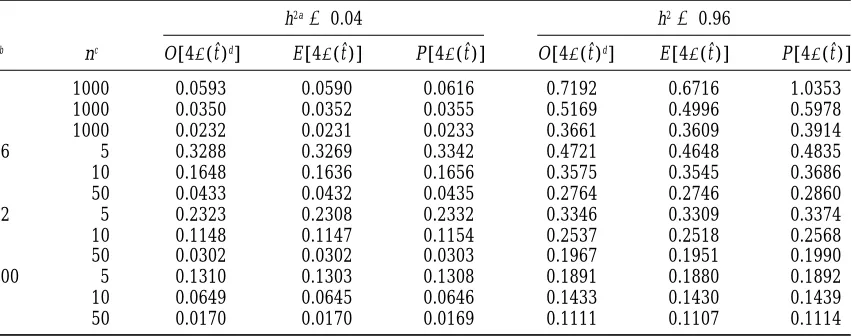
TABLE 1
Observed (O), estimated (E), and predicted (P) standard errors of intraclass correlations
h2a50.04 h250.96
sb nc O[4s(tˆ)d] E [4s(tˆ)] P [4s(tˆ)] O[4s(tˆ)d] E [4s(tˆ)] P [4s(tˆ)]
2 1000 0.0593 0.0590 0.0616 0.7192 0.6716 1.0353
4 1000 0.0350 0.0352 0.0355 0.5169 0.4996 0.5978
8 1000 0.0232 0.0231 0.0233 0.3661 0.3609 0.3914
16 5 0.3288 0.3269 0.3342 0.4721 0.4648 0.4835
10 0.1648 0.1636 0.1656 0.3575 0.3545 0.3686
50 0.0433 0.0432 0.0435 0.2764 0.2746 0.2860
32 5 0.2323 0.2308 0.2332 0.3346 0.3309 0.3374
10 0.1148 0.1147 0.1154 0.2537 0.2518 0.2568
50 0.0302 0.0302 0.0303 0.1967 0.1951 0.1990
100 5 0.1310 0.1303 0.1308 0.1891 0.1880 0.1892
10 0.0649 0.0645 0.0646 0.1433 0.1430 0.1439
50 0.0170 0.0170 0.0169 0.1111 0.1107 0.1114
Estimated standard errors of intraclass correlations were from theOsborneandPaterson(1952) approxima-tion based on 105replicated samples. Standard errors of mean estimates were,0.0002 (h250.04) and,0.002
(h250.96).
aHeritability (four times the intraclass correlation). bNumber of sires.
cNumber of progeny per sire.
dFour times the empirical standard error of the estimated intraclass correlation.
heritability was 1.2619, whereas the predictions from estimates of the heritabilities. Only for large designs are the average estimated and predicted standard errors
Osborne and Paterson (1952) and Fisher (1921)
were 0.2687 and 0.5183, respectively. similar. For powerful designs, i.e., for those designs with a small probability of obtaining least-squares estimates The average estimated standard errors of the
her-itability estimates are close to the observed standard that are out of bounds, the average estimated sampling variance appears to be closer to the observed sampling error from simulation. Clearly, the approximation of
OsborneandPaterson(1952), i.e., the substitution of variance than the predicted values (Table 2).
Relationship between heritability estimates and
sam-the estimated heritabilities into Equation 1, works very
well, and, therefore, using Fisher’s orKempthorne’s pling variance of rg:A more detailed investigation into
the relationship between estimated heritabilities, esti-formula will underestimate the true standard error by
factors of [(s 2 1)/s]1/2 and [(s 2 1)/(s 1 1)]1/2. It mated genetic correlation coefficients, and the
sam-pling variance of the genetic correlation estimate was appears that the average estimated standard error is
closer to the observed standard error than the predic- performed for s5100, n51000, h250.50 (both traits),
and rw5 rg50.75. One million replicated populations
tion using the population values of the heritability.
Sampling variances for genetic correlations: Results were simulated, and both the observed standard error
and the estimated standard error were summarized as are presented in Table 2. Clearly for small n, the
empiri-cal standard error of rg is usually larger than that pre- a function of the geometric mean of the heritability
estimates (i.e., {hˆ13hˆ2}). Simulation results are displayed
dicted under the unconstrained (least-squares) model.
For example, for s 5 100 and n 5 10, the empirical in Figure 1. The graph also includes a plot of the pre-dicted standard error, assuming that the values of the standard error is 0.833 for h250.10 and r
g50.0, whereas
the predicted value is 0.509. When the parameters are heritabilities on the x-axis are the population values. Since for a powerful design with many progeny per sire forced in the parameter space, the maximum empirical
standard error is 1.0, when half of the time an estimate the predicted sampling variance of the genetic correla-tion coefficient does not depend on the heritabilities of 11 is obtained, and half of the time an estimate of
21. For small s and n, the empirical standard error can (Equations 14 and 16), the corresponding line in Figure 1 appears to be horizontal. The prediction of the stan-then be smaller than that predicted. For example, for
s 5100 and n5 2, the empirical standard error from dard error using population values, i.e., h25 0.50 and
rg 5 rw5 0.75, is 0.0443 for this design. The observed
REML was 0.897 for h2 5 0.10 and r
g 5 0, whereas
the predicted value was 2.84. For large n (.10), the standard error of genetic correlation coefficients over all samples, hence also over all possible values of esti-equations perform well. Substituting the estimated
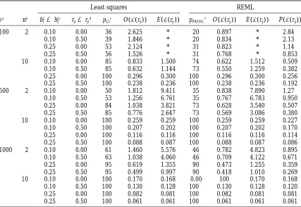
TABLE 2
Empirical (O), estimated (E), and predicted (P) standard errors of estimated genetic correlation coefficients
Least squares REML
sa nb h2
15h22c rg5rpd pLSe O(s(rg)) E (s(rg)) pPREMLf O (s(rg)) E (s(rg)) P (s(rg))
100 2 0.10 0.00 36 2.625 * 20 0.897 * 2.84
0.10 0.50 39 1.846 * 20 0.834 * 2.13
0.25 0.00 53 2.124 * 31 0.823 * 1.14
0.25 0.50 56 1.526 * 31 0.768 * 0.853
10 0.10 0.00 85 0.833 1.500 74 0.622 1.512 0.509
0.10 0.50 85 0.632 1.144 73 0.550 1.259 0.382
0.25 0.00 100 0.296 0.300 100 0.296 0.300 0.256
0.25 0.50 100 0.238 0.236 100 0.238 0.236 0.192
500 2 0.10 0.00 50 1.812 9.411 35 0.838 7.890 1.27
0.10 0.50 53 1.256 6.761 35 0.767 6.783 0.950
0.25 0.00 84 1.038 3.821 73 0.628 3.540 0.507
0.25 0.50 85 0.776 2.647 73 0.569 3.086 0.380
10 0.10 0.00 100 0.259 0.259 100 0.259 0.259 0.227
0.10 0.50 100 0.207 0.202 100 0.207 0.202 0.170
0.25 0.00 100 0.116 0.116 100 0.116 0.116 0.114
0.25 0.50 100 0.088 0.087 100 0.088 0.087 0.086
1000 2 0.10 0.00 61 1.460 5.576 46 0.782 4.823 0.895
0.10 0.50 63 1.038 4.060 46 0.709 4.122 0.671
0.25 0.00 95 0.619 1.355 90 0.473 1.255 0.359
0.25 0.50 95 0.499 0.997 90 0.418 1.010 0.269
10 0.10 0.00 100 0.170 0.168 0.00 100 0.170 0.168
0.10 0.50 100 0.130 0.128 100 0.130 0.128 0.120
0.25 0.00 100 0.082 0.081 100 0.082 0.081 0.081
0.25 0.50 100 0.061 0.061 100 0.061 0.061 0.061
Empirical and estimated standard errors of genetic correlations were estimated from 105replicate populations.
Predicted standard errors were calculated using equations fromTallis(1959) using the population values for the heritabilities and correlation coefficients. An asterisk (*) indicates that the estimate was.10.0.
aNumber of sires.
bNumber of progeny per sire. cHeritability for both traits.
dGenetic and phenotypic correlation coefficient
eProportion (3100) of replicates for which estimates of both sire variances were positive, and the geometric mean of the estimated heritabilities.0.01.
fProportion (3100) of replicates for which the estimated genetic covariance matrix was positive-definite.
ric mean of the heritability estimates was 0.59 (results prediction is very poor. The reason for this is that the distribution of the heritability estimate becomes very not shown).
skewed in these cases, and the Taylor series in Equation 1 ignores higher-order terms by implicitly assuming that DISCUSSION AND CONCLUSIONS both numerator and denominator in the series are nor-mally distributed. In fact, they are distributed
propor-Population or estimated values: It is clear that all
tionally tox2distributions, which are known to be highly
the expressions for the sampling variance of intraclass
skewed for a small number of degrees of freedom [the correlations or genetic correlation coefficients were
es-coefficient of skewness of a centralx2distribution with
sentially derived using a first-order Taylor series about
k degrees of freedom is 23/2/k1/2 (Lancaster 1969, p.
the true population values. Hence, these are the values
20)]. Higher-order Taylor series converged only slowly that should be used to study, for example, the power
(results not shown) and do not improve the prediction of various experimental designs, because they give the
of the sampling variance substantially. For the extreme best prediction of the sampling variance.
case of sires with many progeny it was shown (Equation
Sampling variance of intraclass correlation:The
pre-2) that the predicted standard error of the estimated diction of the sampling variance of the heritability
esti-heritability is proportional to t(1 2 t). However, the
mate based upon population values is accurate for small
observed standard error in this case is a function of t, heritabilities and/or a large number of sires. However,
for a small number of sires and a large heritability, the since (B/ns2
Figure 1.—Standard er-ror of the genetic correla-tion coefficient against the geometric mean of the esti-mated heritabilities, for a design of s5 100 and n5 1000. Population values were 0.50 for the two herita-bilities, and 0.75 for the phenotypic and genetic cor-relation coefficients. Simu-lated results based upon 106
samples. —, predicted val-ues using Equation 14, as-suming that the values on the x-axis are the popula-tion values; – – –, observed standard error; - - -, esti-mated standard error, using the estimated values of the heritabilities and correla-tion coefficients.
series. Hence, theOsborneandPaterson(1952) ap- tables). When this value is used for the standard
predic-tion equapredic-tion (Equapredic-tion 1), the predicted standard er-proximation is biased downward for large heritabilities
and a small number of sires. Although results were not ror of the heritability is 0.5532, which is closer to the observed standard error (0.5169, Table 1) than that shown, the estimate of the heritability is also biased
downward in these cases. However, heritabilities of predicted from the population value of the heritability (0.5978, Table 1).
quantitative traits are not often.0.5, and estimates are
usually based on a reasonable number of families, so Sampling variances of genetic correlations:The ex-pressions for var(rˆg) fromReeve,Tallis, and
Robert-that this problem of an underprediction of the sampling
variance is unlikely to occur. son perform poorly using small population sizes and
small heritabilities when the known population values Estimating the sampling variance of intraclass
correla-tions by substituting the estimates of the heritabilities are used to predict the sampling variance of the genetic correlation coefficient. This is because the estimates of into the standard expressions (OsborneandPaterson
1952) works remarkably well, in that the average esti- the genetic correlation coefficient can become very large (positive or negative) when using least-squares mated standard error is very close to that predicted. For
a large value of the heritability (h250.96) and a small methods. Using REML, the equations perform much
better, although the empirical standard errors are gen-number of sires (s52 or s54), the average estimated
standard error is smaller than the predicted standard erally larger than those predicted in Table 2. Substitut-ing the estimates of the heritabilities and genetic corre-error and appears to be close to the observed standard
error (Table 1). However, further simulations using lations into Equation 15 can result in a very large estimate of the sampling variance of the genetic correla-more extreme values of t showed that this is not a general
observation. For example, for t . 0.5 (corresponding tion when there is a real chance that the estimates of the heritabilities approach zero (the numerator of to “heritability”.2.0) the prediction using population
values is closer to the observed sampling variance than Equation 15 approaches 2/[n(s21)(n21)] for both intraclass correlations approaching zero, whereas the the average estimated sampling variation (results not
shown). Part of the reason why the average estimated denominator goes to zero).
Koots and Gibson (1996) showed in one of their
standard error of the heritability is closer to the observed
sampling variance than the prediction based upon t for simulation studies that the empirical sampling variance of the genetic correlation coefficient depended on the heritability values in the normal range is that it takes
account of the bias in the heritability estimate. Heritabil- estimates of the two heritabilities and concluded that, therefore, the estimates of the heritabilities should be ity estimates are biased downward, in particular for large
values of t and small values of s. For example, for h25 used in, for example, Equation 15, even if the
popula-tion values were known. Further simulapopula-tion results using 0.96, s 5 4, and n 5 1000, the average estimate for
Figure 2.—Standard er-ror of the genetic correla-tion coefficient against the geometric mean of the esti-mated heritabilities, for a design of s5500 and n510. Population values were 0.10 for the two heritabilities, and 0.0 for the phenotypic and genetic correlation co-efficients. —, predicted val-ues using Equation 14, as-suming that the values on the x-axis are the popula-tion values; – – –, observed standard error; - - -, esti-mated standard error, using the estimated values of the heritabilities and correla-tion coefficients.
personal communication) showed very clearly that the served. When the experiment was large and the popula-tion values of the correlapopula-tion coefficients zero, the ob-sampling variance of the genetic correlation coefficient,
conditional on the values of the estimated heritabilities, served and estimated sampling variances, as a function of the geometric mean of the estimated heritabilities, is accurately estimated by substituting the estimated
(and not the true) heritabilities into Equation 15, in were very similar. These additional results confirm the results ofKootsandGibson(1996) and reinforce their
the case of a parent-offspring design, heritabilities of
0.10, and environmental and genetic correlation coeffi- recommendation that the value estimated heritabilities should be used in calculating the sampling variance of cients of zero. This appears to contradict the simulation
results in Table 2, which show that the average sampling the genetic correlation coefficient, even in the rare cases when the population values of the heritabilities are variance is poorly estimated using estimated parameters.
However, the results in Table 2 indicate that the estima- known. From Table 2 it appears that the average esti-mated sampling variance of the genetic correlation coef-tion is poor only when the least-squares estimates are
likely to be outside the parameter space. In the cases ficient is closer to the observed sampling variance than the prediction using population parameters. For one where the least-squares and REML estimates are
identi-cal, both the prediction and average estimated sampling design, s5500, n510, h250.10, r
g5rw50, this was
further explored using the results from 106 replicated
variance are close to the observed one.
The relationship between estimated heritabilities and samples. Figure 2 shows that for hˆ1hˆ2 . 0.07, the
ob-served, estimated, and predicted sampling variance are the empirical sampling variance of the genetic
correla-tion was explored in Figure 1 for a powerful design. virtually identical. For each of the geometric mean classes, the mean estimate of the genetic correlation From these results we may conclude that (1) the
pre-dicted sampling variance accurately predicts the average was zero (results not shown), so that for a particular value of the estimated geometric mean of the heritabilit-observed sampling variance (0.0443), but not the
ob-served sampling variance for given values of the ies, the sampling variance of the genetic correlation coefficients reflects sampling from a population with the achieved estimates of the heritabilities; (2) for a given
value of the estimates of the heritabilities, the estimated true values of the heritabilities equal to those estimated. This is in contrast with the previous example, in which sampling variance follows a very similar pattern to that
of the observed sampling variance (as in Koots and the correlation between the estimated genetic
corre-lation and geometric mean of the heritabilities was
Gibson 1996); (3) for a given value of the estimates
of the heritabilities, the estimated sampling variance is positive (10.59). For smaller values of the estimated heritabilities, Figure 2 shows that the estimated sam-larger than the observed sampling variance; and (4)
when the estimated heritabilities are close to the true pling variance is much larger than either the predicted or observed sampling variance. The estimated sam-values, the predicted and estimated sampling variances
hˆ1hˆ2 5 0.01 was 9.9. It is not clear from these results be biased downward, because of the negative correlation
between the estimate of the heritability and its weight why the average estimated sampling variance is closer
to the observed sampling variance than the prediction (the inverse of the sampling variance). Furthermore, a downward-biased overall heritability estimate would be using population values.
van Vleck andHenderson(1961) investigated the obtained because the heritability estimate from smaller
experiments tends to be biased downward, and the cor-behavior of the expression derived byReeve(1955) for
the parent-offspring regression scenario by simulation. responding estimated sampling variance would be too small, giving too much weight to the smaller experi-They came to the same conclusion asKootsandGibson
(1996); i.e., in the case of a single progeny and one ments. A joint analysis of data, or an iterative procedure, in which the estimated sampling variance for each ex-parent, more than 1000 pairs were needed before
Reeve’s expression was reasonably accurate. periment is recalculated from the pooled heritability
estimate (W. G. Hill, personal communication) is to
Bias in estimate of sampling variance: It is usually
assumed that by substituting the estimates of population be preferred. However, a further complication arises because of a bias in the estimated sampling variance if parameters in the prediction equations for the sampling
variance of the heritability or genetic correlation, unbi- the standard prediction equations are used. This bias may be upward (as shown above) or downward de-ased estimates of those sampling variances are obtained.
However, this is not generally the case for small sample pending on the population parameters. To avoid strong biases in the pooled heritability estimates, a single data sizes. Furthermore, when comparing the average
sam-pling variation from simulation, it matters whether re- analysis should be carried out.
Conclusion:For the design of experimental
popula-sults are expressed in the average standard error (as in
this study) or in the average sampling variance. This is tions to estimate genetic parameters, the prediction of the sampling variance of heritabilities using Osborne
best illustrated using the example of a half-sib design
with large n and a small population value of t. Then andPaterson(1952) is accurate, unless the population
heritability is large and the number of family groups is var(tˆ)5 2t2/(s 21) and s(tˆ) ≈t
√
2/(s21),very small. For analysis of data, the estimate of the stan-dard error of the heritability obtained by substituting with corresponding estimates,
the estimated heritability for the true value in the stan-vaˆr(tˆ) ≈2tˆ2/(s21) and sˆ(tˆ)≈ tˆ
√
2/(s21).dard prediction formulas is almost unbiased for the range of heritabilities and sample sizes likely to be en-If expectations are taken over these estimates, then
countered in practice.
E[vaˆr(tˆ)] 5E[2tˆ2/(s21)]
For small experiments, estimates of heritability are biased downward, and estimates of sampling variances 5(2/(s21))[var(tˆ)1 E2(tˆ)]
are generally not unbiased. Combining results from 5(2/(s21))[2t2/(s2 1)1t2]
different experiments by weighting the heritability esti-mates by the inverse of their estiesti-mates-sampling vari-5var(tˆ)(s11)/(s21)
ances may result in a severely biased heritability
esti-E[sˆ(tˆ)]5E[tˆ ]
√
2/(s21) mate, because the smaller experiments tend to have estimates that are too low, and too much weight is given 5t√
2/(s2 1)5√
(var(tˆ)) .to these estimates if their sampling variances are biased downward too. A joint analysis of all data is to be pre-Hence, for small t and large n, the estimate of the
sam-pling variance can be severely biased upward for a small ferred.
The predicted sampling variance of the genetic corre-number of sires, whereas the estimate of the standard
error is unbiased. It follows that the adjustment of the lation usingReeve(1955) andTallis(1959) are
accu-rate only if the population heritabilities are not close degrees of freedom suggested byKempthorne (1957,
Equation 8) gives an unbiased estimate of the sampling to zero and if the number of families is large. Even if the population heritabilities are known, the estimated variance for small t, but a severely biased estimate of
the standard error. In practice one should therefore be heritabilities should be used in the estimation of the sampling variance of the genetic correlation coefficient. cautious when comparing or using estimated sampling
variances from different experiments. In particular, I thankNaomi WrayandBill Hill for helpful comments and
combining heritability estimates from different-sized ex- Ken KootsandJohn Gibsonfor many constructive discussions and the sharing of additional simulation results.
periments by weighting the estimates proportionally to the inverse of the estimated sampling variance should be avoided because of an induced positive correlation
between the estimate of the heritability and the estimate LITERATURE CITED of its sampling variance, following Equations 1 and 7
Calvin, J. A., 1993 REML estimation in unbalanced multivariate
(W. G. Hill, personal communication). This induced
variance components models using an EM algorithm. Biometrics 49:691–701.
Falconer, D. S., andT. F. C. Mackay, 1996 Introduction to Quantita- Reeve, E. C. R., 1955 The variance of the genetic correlation coeffi-cient. Biometrics 11: 357–374.
tive Genetics. Longman, Harlow, UK.
Fisher, R. A., 1921 On the probable error of a coefficient of correla- Robertson, A., 1959a The sampling variance of the genetic correla-tion coefficient. Biometrics 15: 469–485.
tion deduced from a small sample. Metron 1: 3–32.
Hayes, J. F., andW.G. Hill, 1981 Modification of estimates of Robertson, A., 1959b Experimental design in the evaluation of genetic parameters. Biometrics 15: 219–226.
parameters in the construction of genetic selection indices
(“bending”). Biometrics 34: 429–439. Robertson, A., andI. M. Lerner, 1949 The heritability of all-or-none traits: viability of poultry. Genetics 34: 395–411.
Kempthorne, O., 1957 An Introduction to Genetic Statistics. John
Wiley & Sons, New York. Tallis, G. M., 1959 Sampling errors of genetic correlation coeffi-cients calculated from analyses of variance and covariance. Aust. J. Koots, K. R., andJ. P. Gibson, 1996 Realized sampling variances
of estimates of genetic parameters and the difference between Stat. 1: 35–43.
genetic and phenotypic correlations. Genetics 143: 1409–1416. Taylor, S. C., 1976 Multibreed designs. 1. Variation between breeds. Lancaster, H. O., 1969 The Chi-Squared Distribution. John Wiley & Anim. Prod. 23: 133–144.
Sons, New York. van Vleck, L. D., andC. R. Henderson, 1961 Empirical sampling Meyer, K., andW. G. Hill, 1991 Approximation of sampling vari- estimates of genetic correlations. Biometrics 17: 359–371.
ances and confidence intervals for maximum likelihood estimates Visscher, P. M., 1995 Bias in genetic R2from halfsib designs. Genet. of variance components. J. Anim. Breed. Genet. 109: 264–280. Sel. Evol. 27: 335–345.
Osborne, R., andW. S. B. Paterson, 1952 On the sampling variance Zerbe, G. O., andD. E. Goldgar, 1980 Comparison of intraclass of heritability estimates derived from variance analyses. Proc. R. correlation coefficients with the ratio of two independent F-statis-Soc. Edinb. Sect. B 64: 456–461. tics. Commun. Stat. Theor. Meth. A9: 1641–1655.
Patterson, H. D., andR. Thompson, 1971 Recovery of inter-block