A random model approach to interval mapping of quantitative trait loci.

(1)

A Random

Model

Approach

to Interval

Mapping of

Quantitative

Trait Loci

Shizhong Xu*

and

William

R. Atchley'

*Department of Botany and Plant Sciences, University of California, Riverside, California 92521-0124 and tDepartment of Genetics, North Carolina State University, Raleigh, North Carolina 27695-7614

Manuscript received April 4, 1995 Accepted for publication August 2, 1995

ABSTRACT

Mapping quantitative trait loci in outbred populations is important because many populations of organisms are noninbred. Unfortunately, information about the genetic architecture of the trait may not be available in outbred populations. Thus, the allelic effects of genes can not be estimated with ease. In addition, under linkage equilibrium, marker genotypes provide no information about the genotype of a QTL (our terminology for a single quantitative trait locus is QTL while multiple loci are referred to as QTLs). To circumvent this problem, an interval mapping procedure based on a random model approach is described. Under a random model, instead of estimating the effects, segregating variances of QTLs are estimated by a maximum likelihood method. Estimation of the variance component of a QTL depends on the proportion of genes identical-by-descent (IBD) shared by relatives at the locus, which is predicted by the IBD of two markers flanking the QTL. The marker IBD shared by two relatives are inferred from the observed marker genotypes. The procedure offers an advantage over the regression interval mapping in terms of high power and small estimation errors and provides flexibility for large sibships, irregular pedigree relationships and incorporation of common environmental and fixed effects.

T

HERE are two primary types of data used for mapping a quantitative trait locus (QTL): data derived from inbred lines that include back cross, F2 or more derived populations and field collected data such as those sampled from human populations. With data from line crosses, the parental genotypes, the linkage phases of loci and the number of alleles of the putative QTL are known precisely. In addition, such data from designed experiments can be considered as being from one large family because all individuals share the same parental genotypes. As a result, the effect of QTL substitution and dominance are directly estimated (LANDER and BOSTEIN 1989; HALEY and KNOTT 1992; ZENC

1994). The linear model describing such data is a fixed model. With field data, however, the parental genotypes may not be known. In addition, there will be many different families and the probability of a QTL genotype conditional on a marker genotype will differ from family to family. The linkage phases of parents are usually not known. Although they can be inferred from genotypes of family members, the family size is usually not large enough to allow accurate estimation. As a result, one must try all possible linkage phases and choose the one with the greatest probability (KNOTT and HALEY 1992). Furthermore, the number of alleles of the putative QTL is never known if the origin of the population is unclear. Corresponding to the complicated situation with field data, robust methods, based on a random model approach, were developed (HASE-

Curresponding address Shizhong Xu, Department of Botany and Plant Sciences, University of California, Riverside, CA 925214124, E-mail: [email protected]

Grneticc 141: 1189-1197 (Novernbel-, 1995)

MAN and ELSTON 1972; AMOS and ELSTON 1989; A M O S et al. 1989) where knowledge of the actual genetic model of the QTL is not absolutely required.

Mapping quantitative trait loci with data derived from crosses between two outbred populations is occasionally possible, but these analyses are more difficult than those with other types of data. A population derived from such crosses is in linkage disequilibrium, which violates the assumption required by the random model approach. The uncertainty in the number of alleles and linkage phases of linked loci leads to serious difficulties when a fixed model approach is used. Assuming alterna- tive fixation for QTLs in two diverged outbred lines, the least squares approach (fixed model) of HALEY et al. (1994) for gene mapping can be used. Mapping QTLs in data from crosses between outbred lines has been carried out in pigs by ANDERSON et al. (1994).

(2)

1190 S. Xu and W. R. Atchley However, the genetic variance and linkage parame-

ter are confounded in the Haseman-Elston sib-pair method. A sib-pair interval mapping procedure was recently developed by FULKER and CARDON (1994) using two flanking markers simultaneously to separate these two terms and to locate the quantitative trait locus at a specific position on a chromosome. Although statistical power has been improved, it is still a least squares based method and therefore does not optimally utilize information from the data. GOLDGAR (1990) developed a

multipoint IBD method to estimate the total amount of genetic material shared by relatives in a given chromosomal region and eventually used a maximum likelihood (ML) approach to estimate the genetic variance explained by that particular region. GOLDGAR’S ML is a general method that can be used for any number of sibs or irregular pedigree relationships. This method was extended by SCHORK (1993) to simultaneously estimate variances of several chromosomal regions and the common environment shared by family members. The ML method takes advantage of the distributional property of the data and therefore is more efficient than the Haseman-Elston test (GOLDGAR 1990; GOLDGAR and

ONIKI 1992). Both regression (HASEMAN and ELSTON

1972; FULKER and CARDON 1994) and ML analyses (GOLDGAR 1990) estimate the variance associated with a QTL (or a chromosomal region). Therefore, the models used in these two methods are random models.

SCHORK (1993) and VAN ARENDONK et al. (1994) also

considered the same problem from a mixed model per- spective.

Although GOLDGAR (1990) used two flanking markers to define a chromosomal segment and a ML method to estimate the genetic variance, his method was not designed for interval mapping. Rather, it is intended to test whether at least one QTL is located somewhere in the region. It has been suggested that GOLDGAR’S ML method can be used as a first step in mapping QTLs

(GOLDGAR and ONIKI 1992). When significant variation due to a particular region is detected by GOLDGAR’S method, other approaches could be used to character- ize the specific position of the QTL. If there are large numbers of markers covering the whole genome, the interval flanked by two adjacent markers is expected to be small, e.g., 10 or 15 cM. With a sparse distribution of QTL positions, i.e., there are only a few QTLs randomly distributed along a chromosome, the chance of two QTLs occurring in the same interval may be negligible. In this case, i t is feasible to use GOLDCAR’S ML method for interval mapping. Interval mapping using the ML method will be more efficient than the sib-pair regression method if the distributional properties of the data are known.

The aim of this study is to develop a general QTL mapping procedure using a random model approach (estimating variance) for outbred (random) populations. We extend GOLDGAR’S (1990) ML method to in-

terval mapping and use Monte Carlo simulation to compare the efficiency and statistical power of this new interval mapping procedure with the existing regression mapping (FULKER and CARDON 1994).

THEORY AND METHODS

Herein, we introduce two models: a single QTL model where one QTL is assumed on a tested chromosome and a multiple QTL model where more than one QTLs exist on the tested chromosome.

Single QTL model: The random model is defined

by GOLDGAR (1990) as

= Y

+

g ,

+

( ~ t ,

+

e,, (1)

where yjj is the phenotypic value of the jth member in the zth family, p is the population mean,

g,,

-

N(0, of) is the additive genetic effect (random) of the QTL to be tested on a chromosome, ai,

-

N ( 0 , o:) is the polygenic additive effect (random) and et,

-

N ( 0 , a:) is the environmental deviation. The polygenic term is the summation of effects of all trait loci located on other chromosomes (excluding the putative QTL). Domi- nance effects are ignored here for simplicity. Note that other random effects, such as common environmental effect, can be easily incorporated into the model, but we have chosen this simple model solely to demonstrate the maximum likelihood interval mapping procedure.

The random model is generalized for any pedigree relationship within a family, but to diminish the confu- sion caused by complicated notation for arbitrary pedigree relationships, only full-sibs are considered in this presentation. Under the random model, E(yrj) = 1-1.

Assuming linkage equilibrium, the variance of y4 is Var(y,) =

2

= a%

+

of

+

a: (2)

The coviariance between two noninbred sibs is

Cov(y,,, y $ ) = 7rL7c7;

+

( 3 )

where 7 r i g is the proportion of alleles IBD shared by

family member

j

and

j’

at the putative QTL. The coefficient of the polygenic variance in ( 3 ) is )$ because, by expectation, two noninbred sibs share genes IBD. The IBD of the QTL, 7r+ will be different from one sib-pair to another. This is fundamentally different from the polygenic treatment of a quantitative trait where the IBD value always takes

)$.

If we do not observe or do not have any information about the genotypes of the two sibs for the trait locus, it is natural to replace 7 r j g by its expectation, Le.,

x.

However, the actual 7rz,, is a variable that ranges from 0 to 1.

Let us consider the genotypic configurations of

progenies from the mating type, X AsA4. There are four possible types of progeny, each with an equal frequency. The four possible genotypes are ~ A I A ~ ,

%A,A4, I/4A2A3 and I/4A2A4. If two sibs are sampled from

(3)

possible sib pairs. Suppose we observe two sibs with

AlA3-A1A3. We know they have received exactly the

same alleles from their parents and the IBD is 1. The two sibs behave just like identical twins for this locus. If we observe AIA3-A2&, then we know they do not share any IBD alleles, thus behave like two unrelated individuals. This means that if we happen to know the genotypes of two sibs at a particular locus, the covariance between sibs at this locus conditional on the genotypes may be different from what is expected. For example, Cov(yjf,yg,) = 1 of

+

%a: for a pair of sibs with genotypic configuration of A,A3-A1A, at the QTL and Cov(y,,yj,,) = 0 uf

+

xoz with A1A3-A2A4. It is incorrect to use Cov(yg,yqr ) = &uf

+

xo; if we already know that

j and j ' share no IBD at the QTL.

In practice, genotypes of QTL are not observable. However, we can observe the genotypes of markers linked to the QTLs. HASEMAN and ELSTON (1972) developed the joint probability for two linked loci and showed that the expected IBD of one locus is a linear function of the IBD of another locus. FULKER and CAR-

DON (1994) proposed IBD of two flanking markers to calculate the conditional mean of rj7. The conditional mean of rjq is also a linear function of r s of the two flanking markers (FULKER and CARDON 1994). Let OI2

be the recombination fraction between the flanking markers while

8,q

and 8q2 are recombination fractions between the trait locus and marker 1 and marker 2, respectively. Then

* ; q = E(rqIri1 = a

+

P1rt1

+

P p r z x (4) where 7 r z l and rL2 are the IBD values of the two flanking

markers. FULKER and CARDON (1994) showed

p1

= [ ( I - 28J -

( I

- 28,)*(1 -

2e,,)*i/

[ ( I - ( I -

2&2)41;

p2 = [ ( l - 28f# - (1 - 2O1,)*(1 - 281,)*]1/

[ ( I - ( I - 2012)41;

The term

rj7

in the covariance given in Equation

3 is substituted by this conditional mean

(ei7)

when estimation of variances is performed.

With two sibs in the ith family, for example, the covariance matrix is

where

r; =

*&

+

'/&E

Here we define hf = a$'02 as the heritability of the putative QTL and h: = oE/u2 the heritability of the polygenic effect. Let us first define C, as

If there are k sibs in each family,

C i

is simply a k

x

12 matrix. If normal distribution of the data (y) is assumed, we have the following joint density function of observ- ing a particular vector of data,

where

yi

= [ y i l ,

. . .

,

yEk] 'is a k X 1 vector of phenotypes of the zth sibship and k is the family size, and 1 is a k

x

1 vector with all entries equal to 1. In fact, normal distribution of the QTL effect is not absolutely required as long as the QTL variance is small compared with the sum of the polygenic and environmental variances, but normality of ug and ezI is required to make

yi

normal. The overall log likelihood for n independent families is

n

L =

c

log[f(y,)

1

(8)

i= 1

This likelihood function relates to the position of the trait locus flanked by the two markers through ri. The unknown parameters are p, 0 2 , hi, h: and

el,

Common practice of interval mapping is not maximizing L with respect to all the parameters but first treating B1, as a known constant, then varying

el,

throughout the entire interval, and eventually every interval in the whole genome. The maximum likelihood estimate of the QTL position takes the value of &,in the appropriate interval that maximizes L throughout the entire chromosome. At any particular position in an interval, the algorithm employed here does the following: first, for given prior hi and h:, the maximum likelihood estimates (MLEs) of p and o2 can be expressed as functions of

hi and ht

,

i.e.,

and

If family size varies, nk should be replaced by nkz.

These two equations are obtained by setting the partial derivatives of L with respect to p and o2 equal to zeros, respectively.

(4)

1192 S. Xu and W. R. Atchley

1 1 " 2

L = - - nk lOg(P) - - log( ICil) (11)

2

t = l

Note that after the substitution, p and 0' are absorbed in the likelihood function. We do not treat p and 0' as fixed, rather, we replace them by (9) and

(lo),

respectively. Here we directly maximize (11) with respect to

hi and h: via the simplex algorithm (NELDER and MEAD

1965). It should be noted that substitution of p and 0' by u and u implies that when hi and h: are updated, the two functions, jl = u(hE, h:) and b' = u(hi, h:),

are also updated.

In fact, we can directly use the simplex algorithm to maximize the likelihood function given in (8) with respect to all four parameters ( p , o', hi and h:) simultaneously, but it is computationally inferior because the dimensionality of unknowns will be four instead of two.

Symbolically, let us express Equations 8 and 11 by

L, = function(p, 0 2 , hi, h:) @a) and

&

= function[u(hi, h:), u(hi, h:), h:, h:], ( l l a )

respectively. The algorithm presented here is to maximize

LL

with respect to two parameters ( h i and hz),

which is equivalent to maximizing Ll with respect to four parameters ( p , o', hi and h:)

.

A similar dimension- reduction technique has been used by GRASER et al.

(1987).

The null hypothesis is

H,:hi

= 0, i e . , there is no QTL segregating in the tested interval. The ML under the null hypothesis is denoted by

L.

The likelihood ratio (LR) test statistic is

LR = -2(Lo - L l ) (12)

which follows a chi-square distribution with 2 2 d.f.

>

1 under H , . One degree of freedom is due to fitting

hi and the remaining degree of freedom is for fitting the QTL position (HALEY and KNOTT 1992). For a given interval, the remaining degree of freedom depends on the size of the interval

(el2)

and it is less than one because we only search the QTL within the tested interval, rather than the entire genome. If the null hypothe-

sis is no QTL in the whole genome (notjust one interval) covered by the markers, then df

=

2

under the null hypothesis. With many markers on a long chromosome, the number of degrees could be greater than two

(ZENG 1994) for a chromosomal wise test.

Multiple QTL model: The above model assumes

there is only one QTL in the linkage group where the tested interval is located. If there are multiple QTLs in the same linkage group, the estimation tends to be bi- ased because of interference caused by QTLs located on the same chromosome but outside the tested interval (HALEY and KNOTT 1992; MARTINEZ and CURNOW 1992;

JANSEN 1993, 1994; ZENG 1993, 1994). The multiple QTL model is described by

S W

yq = p

+

aij

+

ut.+

g;,

+

u;

+

e,j (13)

where ut and ub are the kth QTL effect on the left side and the 7th QTL effect on the right side of the putative QTL, 5' and Ware the numbers of trait loci in the left and right sides of the current QTL. Under the assumption of linkage equilibrium, the variance of ye is

k= I F l

Y W

Var(y,) = 0' =

CT:

+

x

0:

+

ui

+

CT:

+

a: (14)

k= 1

and the covariance between noninbred sibs is

r - l

r W

cov(yj/j ri/') =

&

0:

+

Tiq0:

+

Tj,a: (15)

k= 1 ,= I

Note that these 7rs are the IBD proportions of the QTLs, and they are not observable.

SCHORK (1993) proposed a similar model and suggested to include more chromosomal regions into the conditional covariance for purpose other than interval mapping. Theoretically, we can define the conditional covariance given the 7rs of all markers in the linkage group and include all variance components explained by each marker into the likelihood function to control other QTL effects. However, technically this is not feasible because of so many variance components and also it is not necessary. The IBD variable has the same property as the indicator variables ( ZENG 1993) in that conditional on the 7r of a marker locus, the 7r of a QTL on one side of the marker is not correlated to that of a QTL on the other side. This will become evident when we reexamine Equation 5 by treating the QTL as a neutral marker. Let us define the two flanking markers and the QTL by i,

j

and k, respectively. Equation 5 is then rewritten as

pl

ZZ [ ( I - 28jk)2 - (1 - 28kj)'(1 - 28,)2]/

[ ( I - (1 - 28tj)41;

p2 = [ ( I - 28,)' - (1 - 28jk)*(1 - 28,)2]/

[ ( I - (1 - 2 0 4 ~ 1

This equation holds regardless of the order the three loci are arranged on the chromosome. If the order is i

<

k

<

j , this equation is required to predict T k . How-

ever, if the order is k

<

i

<

j ,

then (1 - 28jk)' = (1 -

28jk)'(1 - 28,)', which leads to

p1

= (1 - 28,k)' and

p2

= 0. On the other hand, if i

<

j

<

k, then (1 - 2 8 i k ) ' = (1 - 28,,)'(1 - 28,)' leading to = O and

(5)

ZENG (1994) for the indicator variables. The only difference is that the indicator variables are observed without error while the IBD proportions are estimated with some uncertainty if the mating type is not fully informative.

These properties are the bases of the composite interval mapping of ZENG (1993, 1994) and JANSEN (1993, 1994) for line cross populations, which will be directly adopted here for the random model approach. Theo- retically, one marker is enough to block correlation between a locus on the left and a locus on the right. Therefore, we only need two additional markers flanking the current interval to block interference caused by outside QTLs. Here we still use markers 1 and 2 to denote the two flanking markers that define the tested interval, but use L and R to denote the next-to-flanking markers. Now the four markers have the order: L

-

1

-

2

-

R

The tested QTL is between markers 1 and 2. Let T ~and riIt ~ , be the IBD values of the left ( L ) and right (R) additional markers, respectively, and Okl. and

OrR be the recombination fractions of the kth QTL with locus L and the rth QTL with locus

R

Given the four markers the conditional covariance between sibs is

COv(yi1, JB

I

T l l . * i v r d

= a2[[nll.H;,

+

?tiqh:

+

T R H ; ~

+

%hz] (16)

where H;- =

E;==,,

(1

-

2O&)'hi, H;, =

E

:

,

(1 -

20:R)2h:, hi =

a:/a'

and h: =

o:/a'.

At a particular position, the parameters in the likelihood function are

p, a2, H;., hi, HYt and hz, but only h: is tested.

The computing algorithm follows that for single QTL model, but now there are more unknown variance components. The solutions of the unknowns must be searched within the appropriate solution space, other- wise the covariance matrix is not assured to be positive definite. A method of reparameterization described in the APPENDIX is used to obtain a positive definite covariance matrix and thus guarantee convergence to a solution.

There will be some interference if QTLs exist between markers L and l or Rand 2. However, under the assumption of a dense marker map and a few QTLs randomly distributed along a chromosome, there may be small chance of two QTLs existing in two adjacent intervals. Theoretically, the tests of different intervals are independent

(ZENC

1993), though independence may not be guaranteed with small population sizes.

The multiple QTL method has both advantages and disadvantages when compared with the single QTL one. The advantage is when the other intervals do contain QTLs whose effects can then be absorbed by the next- to-flanking markers. The disadvantage is when there is no QTL in the other intervals, in which case we loose power because the next-to-flanking markers will pick up random noise instead of QTL effects. In other words,

v

x:

-

x;

-

LR5 -

LR3

-

95 percentile

, , , , , , , ( , , Lu

100

80

60

40

20

0

- 0 1 2 3 4 5 6 7 8 9 f O 1 1 1 2 1 3 -

LR

test

statistc

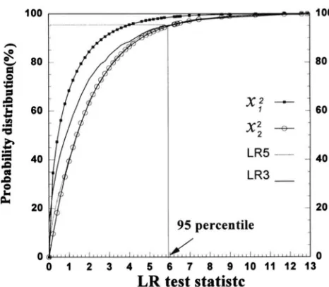
FIGURE 1.-Empirical cumulative distributions of the likelihood ratio (LR) test statistic. The curve is compared with the distributions of

x&=,

and

x.$=2.

by using the multiple QTL model we may gain accuracy at the price of loosing power.

SIMULATION STUDIES

Test statistic under the null hypothesis: To further

investigate the behavior and the threshold value of the test statistic of the ML method, we simulated data under the null hypothesis of no QTL on the tested chromosome. Under the null hypothesis, we simulated the polygenic effect with a heritability of 0.5. Six codominant markers each with six equally frequent alleles were simulated. The six markers were linked 20 cM apart and covered a linkage group of 100 cM length. The IBD values of markers were calculated using the method of HASEMAN and ELSTON (1972). Five hundred independent full-sib families, each with two sibs, were simulated in each experiment. The simulation experiment was repeated 1000 times. In each experiment, the maximum LR of the single QTL model was recorded throughout the entire chromosomal segment. The empirical distribution of the LR test statistic over 1000 replicates was examined and shown in Figure 1. The 95th percentile of the empirical distribution was 5.85. This figure also gives two chi-square distributions with 1 and 2 d.f., respectively. The empirical LR test statistic has a distribution almost indistinguishable from the distribution. Therefore, the critical value of 5.99

(=

x : . ~ ~ ( ~ ) )

was used to determine the level of signifi-

cance in subsequent simulation studies.

To compare our method with FULKER and CARDON'S

(6)

1194 S. Xu and W. R. Atchley

FULKER and CARDON (1994) was -1.856 for an inter- valwise test. Because we were interested in chromo- somewise test, the critical value -2.448 was used in this study. Note that the t statistic is approximately the square root of

x&=‘

under the null hypothesis. This becomes obvious by looking at (-2.448)‘ = 5.993, which is virtually identical to the critical value of distribution. Therefore, instead of t, the

t2

test statistic was used for the sib-pair regression analysis. Before con- verting t into t‘ statistic, we replaced any positive value of t by 0 so that the t‘ test is still a one-tail test. In subsequent analyses, the threshold value of 5.99 was used for both the LR and t‘ tests.

Experimental design: Extensive simulation was done

on the single QTL model. The genetic model is as follows: there was one QTL with either two or six allelic states of equal frequency. The allelic effects were set such that the additive variance explained by the QTL was 12.5 squared units. Dominance effect was assumed to be absent. No polygenic effect was simulated, but t.he polygenic term was fitted in the model when the ML method was used. Heritability was set at 0.25 and 0.50 by adjusting the amount of random environmental deviation assigned to the phenotype. Six codominant markers each with six alleles of equal frequency were simulated. The six markers were linked 20 cM apart and covered a linkage group of 100 cM length. The simulated QTL was located in the middle of the chromosome segment, i.e., 50 cM. Two sibs in each family were simulated, and the number of families (sample size) varied at 250, 500 and 1000. In each set of parameter combination, the simulation was repeated 100 times.

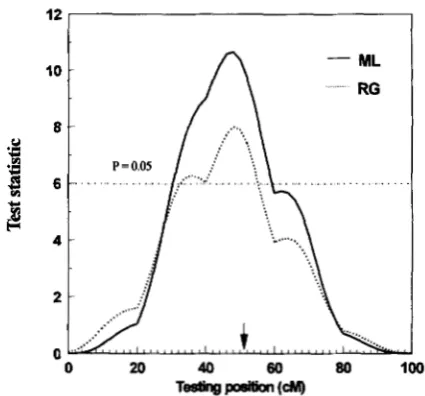
Results: Result from a single replicate of simulation

was depicted in Figure 2, where the parameters were: heritability = 0.50, number of alleles = 2, sample size

= 500. The test statistic of the ML method was compared with that of the regression (RG) method, showing that the LR profile had a higher peak than the t2 profile. Mean estimates and standard deviations (over 100 replicates) of the QTI, location (cMA), variance explained by the QTL

(ai)

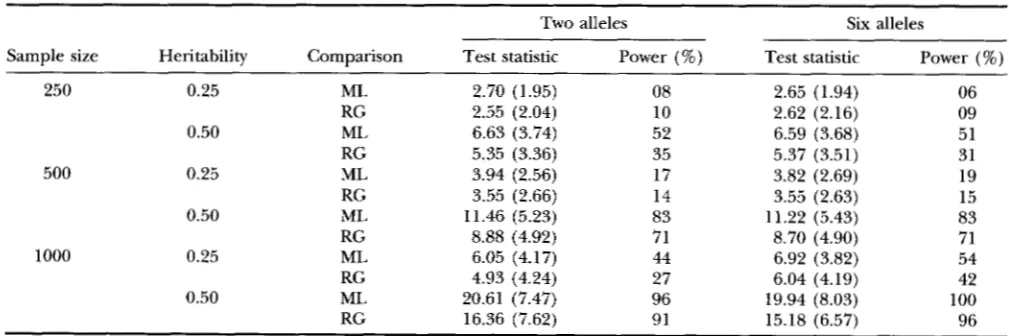
and the polygenic variance

(a:) are summarized in Table 1, which demonstrates:

(1) the number of alleles in the QTL had little influ- ence on estimation of both methods; (2) standard deviations of parameter estimates in ML were smaller than those in the regression method, ie., ML had smaller estimation errors than RG; and (3) QTL variance was overestimated by the regression method, especially when heritability and sample size were small.

Clearly, the maximum likelihood method performs much better that the regression method.

It is well known that the regression method generates unbiased estimates of regression coefficients. At first glance it might seem that estimation of the QTL variance should be unbiased with the regression method because it is estimated by a term proportional to the

12 _I

I

Y

0 20 40 60 80 loo

T d w (CM)

FIGURE 2.-Comparison of the LR profile of maximum likelihood (ML, -) with the ? statistic profile of regression (RG, *

.

*

.

) drawn from a single simulation experiment of

500 full-sib families each with two members. The QTL is lo-

cated at 50 cM, has two alleles and explains 50% of the total phenotypic variation.

regression coefficient. However, the property of unbi- asedness only holds when the QTL position is fixed. If the QTL location varies, then the variance associated with the QTL tends to be overestimated because the method always chooses a location with the highest t’

that is proportional to the squared QTL variance. The average test statistics and power estimates (at a

= 0.05) over 100 replicates are summarized in Table 2.

The test statistics were likelihood ratio (LR) for the ML method and

?

for RG method, both having a critical value of 5.99 under the null hypothesis. The ML method in general has a higher statistical power than the regression method.

Multiple QTL model: Because intensive computa-

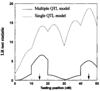
tion is involved for the multiple QTL model, we only simulated one sample of 1000 sib-pairs for the multiple QTL model to demonstrate the behavior of the LR profile. More extensive simulation is left for a later paper. In this paper, we simulated two QTLs located in the 15 and 45 cM positions on a linkage group of size 50 cM. The two QTLs have an equal effect on the trait with a total heritability of 0.5. The result from the multiple QTL model was compared with that of the single QTL model. These LR profiles are shown in Figure 3.

The multiple QTL model clearly indicates two QTLs at the correct positions while the single QTL model shows two major peaks, but each with two subpeaks. The two subpeaks in the middle are the “ghost images” (HALEY

(7)

TABLE 1

Comparison of maximum likelihood and regression analyses of simulated data

Sample Two alleles Six alleles

size Heritability Comparison CMA

e;

8

CMA

e:, e:

250 0.25 ML 49.66 (26.61) 12.64 (5.39) 1.61 (4.16) 49.90 (27.02) 12.54 (5.19) 1.63 (3.88) RG 49.84 (28.48) 21.36 (11.09)

-

52.00 (28.16) 21.56 (11.71)

0.50 ML 49.44 (19.15) 11.56 (2.97) 1.99 (3.09) 50.98 (19.08) 11.69 (2.91) 1.36 (2.74) RG 49.10 (19.58) 14.35 (5.65)

-

52.74 (19.62) 14.63 (5.66)

500 0.25 ML 46.12 (24.53) 12.05 (4.25) 1.53 (3.33) 48.46 (23.43) 11.78 (4.34) 1.54 (3.43) RG 45.02 (26.85) 18.04 (8.41)

-

46.18 (26.43) 17.94 (8.52)

0.50 ML 49.32 (12.64) 11.67 (2.45) 1.20 (2.23) 51.94 (14.42) 11.55 (2.49) 1.12 (2.17) RG 50.74 (14.04) 13.75 (4.33)

-

49.18 (15.30) 13.69 (4.43)

RG 45.92 (24.04) 15.48 (7.29)

-

51.80 (23.19) 17.91 (6.94) -

RG 49.42 (8.15) 13.60 (3.55)

-

46.86 (11.80) 13.49 (3.33)

-

1000 0.25 ML 46.62 (23.77) 11.34 (3.57) 1.74 (3.18) 53.28 (20.28) 12.26 (3.37) 1.27 (2.94)

-

0.50 ML 49.26 (6.36) 11.83 (1.85) 0.68 (1.44) 48.60 (8.68) 11.59 (1.76) 0.94 (1.68)

ML, maximum likelihood; RG, regression; cM,, QTL location; 6:; variance explained by the QTL;

e:,

polygenic variance. The standard deviations of the estimates over 100 replicates are given In parentheses. The true location (cMA) and QTL variance

(ai)

are 50 cM and 12.5 squared units, respectively, while the true polygenic variance is zero.

If we had used the critical value from the single QTL rectly estimates the QTL effect. The ML and regression model, the power would have been reduced with the compared in this study deal with a random model that multiple QTL model. By using the multiple QTL estimates the QTL variance. Under some circum- model, we may gain accuracy at the cost of power. Simi- stances, e.g., the QTL being at one flanking marker, lar results are present in the composite interval map- estimates of the QTL effect by the regression and ML ping procedures of ZENG (1994). are equivalent under the fixed model. If the QTL is not at a flanking marker, the difference is expected to be

DISCUSSION negligible if the QTL effect is small relative to the residual standard deviation. Therefore, regression mapping Recent studies that compare ML with regression in _{is an}_{approx~mat~on}_of_ML_{mapping under} _{a fixed}

line find no difference between the _{model. In contrast to the fixed model, random model} methods

(mEY

and

lg92;

and _{regression mapping is not an approximation}_of_{ML un-}

cumow

1992). At first glance it might Seem that Our _{der any circumstances. The two methods may generate} ML should not be significantly different from F U L m R _{similar results if sample sizes are large, but there} _is

and CARDON'S (1994) regression. However, the ML and no mathematical basis for any equivalence. The higher regression compared by HALEY and K N O n (1992) and power of ML compared with regression is probably due others are based on a fixed model approach that di- to the fact that ML uses the phenotypic values as the

TABLE 2

Comparison of statistical powers between maximum likelihood and regression analyses of simulated data

Two alleles Six alleles

Sample size Heritability Comparison Test statistic Power (%) Test statistic Power (%)

250 0.25 ML _{2.70 (1.95)} 08 2.65 (1.94) 06

RG _{2.55 (2.04)} 10 2.62 (2.16) 09

0.50 ML _{6.63 (3.74)} 52 6.59 (3.68) 51

RG _{5.35 (3.36)} 35 5.37 (3.51) 31

500 0.25 ML _{3.94 (2.56)} 17 3.82 (2.69) 19

RG 3.55 (2.66) 14 3.55 (2.63) 15

0.50 ML _{11.46 (5.23)} ₈₃ _{11.22 (5.43)} ₈₃

RG 8.88 (4.92) 71 8.70 (4.90) 71

RG _{4.93 (4.24)} 27 6.04 (4.19) 42

0.50 ML _{20.61 (7.47)} 96 19.94 (8.03) 100

RG _{16.36 (7.62)} 91 15.18 (6.57) 96

1000 0.25 ML 6.05 (4.17) 44 6.92 (3.82) 54

(8)

1196 S. Xu and W. R. Atchley

Multiple QTL model

. . Single QTL model

15 _.... : .

.

. . . . ::

....

0 10 20 30 40 50

TesUng position

(a)

FIGURE S.-Comparison of the LR profile of the multiple QTL model (-) with that of the single QTL one ( *

-

* ).

Results were drawn from a single simulation experiment of

1000 full-sib families each with two members. The two QTLs,

accounting for 50% of the total phenotypic variation, are located at 15 cM and 45 cM positions with an equal effect.

raw data and takes advantage of the property of normal distribution, whereas the regression uses the squared phenotypic differences as the raw data. As a conse- quence, property of normal distribution is not utilized and also some information may have been lost.

The question now is how to calculate the proportion of genes shared IBD. If the parental mating type of the sibs are known, it is relatively easy to obtain the T S for all possible sib-pairs. However, this is difficult if the parental genotypes are unknown. However, given the allelic frequencies of the marker locus and assuming H-W equilibrium, the T S can be estimated. In both situa- tions, the proportions of genes shared IBD between sibs are given in HASEMAN and ELSTON (1972). The proportions of genes IBD shared by half-sibs and other types of relatives in a complicated pedigree are usually estimated using a maximum likelihood approach (see

A M O S et al. 1990). In this paper, we do not attempt to estimate the m , rather we assume that the n-s are known

and thus focus on mapping procedures using these T values.

We have borrowed ZENG'S (1994) idea of composite interval mapping for the multiple QTL model where we can treat genotypes of other markers outside the tested interval as fixed effects to control the genetic background. The problem here is that at linkage equilibrium the conditional probability of a QTL genotype given a marker genotype will remain unchanged in the whole population, leading to zero regression coefficients for all the marker genotypes. In fact, we must treat marker genotypes as nested within each family, which will increase the levels of the fixed effect. For instance, if all markers are fully informative, potentially there will be four genotypes per marker within each

family. In the whole population, the number of levels for each marker may be up to 4n, where n is the number of families. Unless there are a few families and each has large number of members, we can not simultaneously put all marker genotypes into the model. There- fore, the four marker approach in our multiple QTL model is appropriate.

The regression interval mapping of FULKER and CAR-

DON (1994) still offers an advantage over the ML method in terms of computing speed. Hypothesis testing with a computationally fast algorithm can be easily accomplished by a recently developed permutation test method (CHURCHILL and DOERGE 1994) when an exact test is not available. In addition, the idea of composite interval mapping of ZENC (1994) and JANSEN (1994) can be directly adopted to FULKER and CARDON'S (1994) mapping procedure by simply incorporating the IBD values of other important markers to control the genetic background and reduce the residual variance. To select important markers, one should ConsultJANsEN

(1994).

One major advantage of using ML over regression is that the ML presents no difficulty for large sibships and irregular pedigree relationships. Although extension has been made to include large and complicated pedigrees by using weighted or generalized least squares methods (BLACKWELDER and ELSTON 1982; OLSON and WIJSMAN 1993), the methods still represent ad hoc approaches in terms of statistical testing, because the data (squared differences) are not normally distributed. In addition, the ML method presents no problem in incorporating fixed effects into the model to control the residual variance (SCHORK 1993). For such a mixed model, variance components are easily estimated using the well developed restricted maximum likelihood (REML) programs (e.g., MEYER 1988). Upon incorporation of the interval mapping procedure into REML programs, QTL mapping in livestock and human populations will become routine. It is not feasible to use the ML method for extensive simulation studies due to pro- hibited computing load, but it can be widely used in real data analyses.

We are deeply indebted to Professors WII.I.IAM M. MUIR and ZHAO- BANG ZENC for helpful comments on an earlier version of the manuscript. We also want to acknowledge Professor SURIR GHOSH for evalu- ating the ML algorithm presented in the manuscript. The current work was supported by National Institutes of' Health grant GM-45344 and National Science Foundation grant BSR-910718.

LITERATURE CITED

A M O S , C. I., and R. C. ELSTON, 1989 Robust methods for the detec-

tion of genetic linkage for quantitative data from pedigrees. Genet. Epidemiol. 6 349-360.

A M O S , C. I., R. C. EISTON, A. F. WILSON and J. E. VNLEYWII.SON,

1989 A more powerful robust sib-pair test of linkage for quanti-

A M O S , C. I., D. V. DAWSON and R. C. ELSTON, 1990 The probabilistic

tative traits. Genet. Epidemiol. 6: 435-449.

(9)

ANDERSON, L., C. S. HALEY, H. ELLEGREN, S. A. KNOW, M. JOHANSSON

et aZ., 1994 Genetic mapping of quantitative trait loci for growth and fatness in pigs. Science 2 6 3 1771-1774.

BLACKWEI.DER, W. C., and R. C. ELSTON, 1982 Power and robustness of sibpair linkage tests and extension to larger sibships. Com- mun. Statist. Theor. Methods 11: 449-484.

BISHOP, D. T., and J. A. WILLIAMSON, 1990 The power of identity- by-state methods for linkage analysis. Am. J. Hum. Genet. 4 6 CHURCHIIL, G . A., and R. W. DOERGE, 1994 Empirical threshold

values for quantitative trait mapping. Genetics 138: 963-971. DEGROOT, M. H., 1986 Probability and Statistics, Ed. 2. Addison-Wes-

ley Publishing Company, Reading, MA.

FUI.KER, D. W., and L. R. CARDON, 1994 A sib-pair approach to interval mapping of quantitative trait loci. Am. J. Hum. Genet. 5 4 : 1092-1103.

GOLDGAR, D. E., 1990 Multipoint analysis of human quantitative genetic variation. Am. J. Hum. Genet. 47: 957-967.

GOIDGAR, D. E., and R. S. ONIKI, 1992 Comparison of a multipoint identity-by-state method with parametric multipoint linkage analysis for mapping quantitative traits. Am. J. Hum. Genet. 5 0 598-606. GRMER, H.-U., S. P. SMITH and B. TIER, 1987 A derivative-free a p

proach for estimating variance components in animal models by restricted maximum likelihood. J. h i m . Sci. 64: 1363-1370. HALEY, C. S., and S. A. W o n , 1992 A simple regression method

for mapping quantitative trait loci in line crosses using flanking markers. Heredity 69: 315-324.

HALEY, C. S, S. A. KNOTT and J.-M. ELSEN, 1994 Mapping quantitative trait loci in crosses between outbred lines using least squares. Genetics 136: 1195-1207.

HASEMAN, J. K., and R. C. ELSTON, 1972 The investigation of linkage between a quantitative trait and a marker locus. Behav. Genet.

2 3-19.

JANSEN, R. C., 1993 Interval mapping of multiple quantitative trait loci. Genetics 135: 205-211.

JANSEN, R. C., 1994 Controlling the Type I and Type I1 errors in mapping quantitative trait loci. Genetics 138: 871-881.

KNOTT, S. A, and C. S. HALEY, 1992 Maximum likelihood mapping of quantitative trait loci using fullsib families. Genetics 132: 1211-1222.

LANDER, E. S., and D. BOSTEIN, 1989 Mapping Mendelian factors underlying quantitative traits using RFLP linkage maps. Genetics 121: 185-199.

MARTINEZ, O., and R. N. CURNOW, 1992 Estimating the locations and the sizes of the effects of quantitative trait loci using flanking markers. Theor. Appl. Genet. 85: 480-488.

MEYER, R, 1988 DFREML-a set of programs to estimate variance components under an individual animal model. J. Dairy Sci. 71: 33-34.

NELDER, J. A,, and R. MEAD, 1965 A simplex method for function minimization. Comput. J. 7: 308-313.

OLSON, J. M., and E. M. WIJSMAN, 1993 Linkage between quantitative trait and markers loci: methods using all relative pairs. Genet. Epidemiol. 1 0 87-102.

SAS Institute Inc., 1988 SAS/STAT User’s G u i d e , Release 6.03. SAS Institute Inc., Cary, NC.

SCHORK, N. J., 1993 Extended multipoint identity-bydescent analysis of human quantitative traits: efficiency, power, and modeling considerations. A m . J. Hum. Genet. 53: 1306-1393.

VAN ARENDONK, J. A. M., B. TIER and B. P. KINGHORN, 1994 Use of multiple genetic markers in prediction of breeding values. Genetics 137: 319-329.

ZENG, Z.-B., 1993 Theoretical basis for separation of multiple linked gene effects in mapping quantitative trait loci. Proc. Natl. Acad. Sci. USA. 90: 10972-10976.

ZENG, Z.-B., 1994 Precision mapping of quantitative trait loci. Genet- ics 136 1457-1468.

254-265.

Communicating editor: P. D. KEICHTLEY

APPENDIX

A method of reparameterization is described here to ensure the simplex algorithm to search the unknowns

in the appropriate solution space. Recall that the conditional covariance is Cov(yil,yi21 7 r & i g 7 r i K ) = a‘r,, where

r, =

TLG,

+

T,,hi

+

T ; E P R

+

xh: The permissible space of the heritabilities is

l r H ~ ~ O , l r h ~ ~ O , l ~ ~ K r O , l ~ h ~ ~ O ,

and 1 z h2 2 0

where h2 =

#,

+

hi

+

PR

+

hi is the overall heritability. These various heritabilities have to be searched within this space to guarantee a positive definite covariance matrix. Although we could borrow a technique of non- linear programming from operations research that maximizes the likelihood function subject to these con- straints, in this particular situation, we found that it is easier to use a method of reparameterization. The method of reparameterization is justified by the invari- ance property of the maximum likelihood estimators

(DEGROOT 1986, p. 348). Defining y1 = @,/h2, y 2 =

hi/h2 and yy =

pR/

h2 and y 4 = h:/h2, we have

ri = [TzLyl

+

f i z q 7 2

+

‘ I T i R 7 3

+

%y41h2

We now have five unknowns with a permissible space defined by

1 z h 2 z 0 , ~ y z = 1 and y i r O f o r i = l ,

. . . ,

4

i= 1

These newly defined terms can be reparameterized as

h2 = e x p b ) _and y i =

1

+

exp(z) Zf= exp ( x,)

exp ( xi)

f o r i = 1,

. . . ,

4

where z and x, are any real numerals without any con- straints. Instead of maximizing the likelihood function

( L ) with respect to ys and h2, we will maximize L with respect to these xs and z. Let gi and i denote the ML

estimates of xi and z, then the ML estimates of the original heritabilities are

p

= exp(8 fi;, =

p

exp ( 21

1

+

exp(2) ’

Z f z l

exp(2,) ’