A Two-Channel Training Algorithm for Hidden Markov Model and Its Application to Lip Reading

A Two-Channel Training Algorithm for Hidden Markov

Model and Its Application to Lip Reading

Liang Dong

Department of Electrical and Computer Engineering, National University of Singapore, Singapore 119260 Email:[email protected]

Say Wei Foo

School of Electrical and Electronic Engineering, Nanyang Technological University, 50 Nanyang Avenue, Singapore 639798 Email:[email protected]

Yong Lian

Department of Electrical and Computer Engineering, National University of Singapore, Singapore 119260 Email:[email protected]

Received 1 November 2003; Revised 12 May 2004

Hidden Markov model (HMM) has been a popular mathematical approach for sequence classification such as speech recognition since 1980s. In this paper, a novel two-channel training strategy is proposed for discriminative training of HMM. For the proposed training strategy, a novel separable-distance function that measures the difference between a pair of training samples is adopted as the criterion function. The symbol emission matrix of an HMM is split into two channels: a static channel to maintain the validity of the HMM and a dynamic channel that is modified to maximize the separable distance. The parameters of the two-channel HMM are estimated by iterative application of expectation-maximization (EM) operations. As an example of the application of the novel approach, a hierarchical speaker-dependent visual speech recognition system is trained using the two-channel HMMs. Results of experiments on identifying a group of confusable visemes indicate that the proposed approach is able to increase the recognition accuracy by an average of 20% compared with the conventional HMMs that are trained with the Baum-Welch estimation.

Keywords and phrases:viseme recognition, two-channel hidden Markov model, discriminative training, separable-distance func-tion.

1. INTRODUCTION

The focus of most automatic speech recognition techniques is on the spoken sounds alone. If the speaking environment is noise free and the recognition engine is well configured, high recognition rate is attainable for most speakers. How-ever, in real-world environments such as office, bus station, shop, and factory, the speech captured may be greatly pol-luted by background noise and cross-speaker noise. Present-ing such a signal to a sound-based speech recognition sys-tem, the recognition accuracy may drop dramatically. One solution to enhance the speech recognition accuracy under noisy conditions is to jointly process information from mul-tiple modalities of speech. Automatic lip reading is one mode in which the visual aspect of speech is considered for speech recognition.

It has long been observed that the presence of visual cues such as the movement of lips, facial muscles, teeth, and tongue may enhance human speech perception. Systematic studies on lip reading have been carried out since 1950s [1,2,

3,4,5,6,7,8,9,10,11,12,13,14,15,16,17]. Sumby and Pol-lack [1] showed that the incorporation of visual information added an equivalent 12 dB gain in signal-to-noise ratio.

Among the various techniques for visual speech recog-nition, hidden Markov model (HMM) holds the greatest promise due to its capabilities in modeling and analyzing temporal processes as reported in [9,18,19,20,21,22,23,

24,25,26,27,28,29]. Most of the HMM-based visual speech processing systems reported take an individual word as the basic recognition unit and an HMM is trained to model it. Such an approach works well with limited vocabulary such as digit set [15,30], a small number ofAVletters[31], and isolated words or nonsense words [32], but it is difficult to

The smallest visibly distinguishable unit of visual speech is commonly referred to as viseme [33]. Like phonemes that are the basic building blocks of sound of a language, visemes are the basic constituents for the visual representa-tion of words. The time variarepresenta-tion of mouth shape in speech is small compared with the corresponding variation of acoustic waveform. Some previous experiments indicate that the tra-ditional HMM classifiers, which are trained with the Baum-Welch algorithm, are sometimes incompetent to separate mouth shapes with small difference [34]. Such small dif-ference has prompted some researchers to regard the rela-tionship between phonemes and visemes as many-to-one mapping. For example, although phonemes /b/, /m/, /p/ are acoustically distinguishable, the sequence of mouth shape for the three sounds are not readily distinguishable, hence the three phonemes are grouped into one viseme category. An early viseme grouping was suggested by Binnie et al. [35]. The MPEG-4 multimedia standard adopted the same viseme grouping strategy for face animation, in which four-teen viseme groups are included [36]. However, different

groupings are adopted by different researchers to fulfill spe-cific requirements [37,38].

Motivated by the need to find an approach to diff erenti-ate visemes that are only slightly different, we propose a novel approach to improve the discriminative power of the HMM classifiers. The approach aims at amplifying the separable-distance between a pair of training samples. A two-channel HMM is developed, one channel, called the static channel, is kept fixed to maintain the validity of the probabilistic frame-work, and the other channel, called the dynamic channel, is modified to amplify the difference between the training pair. A hierarchical classifier is also proposed based on the two-channel training strategy. At the top level, broad identi-fication is performed and fine identiidenti-fication is subsequently carried out within the broad category identified. Experi-mental results indicate that the proposed classifier excels the traditional ML HMM classifier in identifying the mouth shapes.

Although the proposed method is developed for the recognition of visemes, it can also be applied to any sequence classification problem. As such, the theoretical background and the training strategy of the two-channel discriminative training method are introduced first in Sections 2,3, and

4. This is followed by discussion of the general properties and extensions of the training strategy in Sections 5 and

6, respectively. Details of the application of the method to viseme recognition and the experimental results obtained are given inSection 7. The concluding remarks are presented in

Section 8.

2. REVIEW OF HIDDEN MARKOV MODEL

Hidden Markov model is also referred to as hidden Markov process (HMP) as the latter emphasizes the stochastic process rather than the model itself. HMP was first introduced by Baum and Petrie [39] in 1966. The basic theories/properties of HMP were introduced in full generality in a series of pa-pers by Baum and his colleagues [40, 41, 42, 43], which

include the convergence of the entropy function of an HMP, the computation of the conditional probability, and the local convergence of the maximal likelihood (ML) parameter esti-mation of HMM. Application of HMM to speech processing took place in the mid-1970s. A phonetic speech recognition system that adopts HMM-based classifier was first developed in IBM [44,45]. Applications of HMM for speech processing were further explored by Rabiner and Juang [46,47].

The beauty of HMM is that it is able to reveal the under-lying process of signal generation even though the properties of the signal source remain greatly unknown. Assume that

OM _{= {O}

1,O2,. . .,OM}is the discrete set of observed

sym-bols andSN_{= {S}

1,S2,. . .,SN}is the set of states; anN -state-M-symbol discrete HMMθ(π,A,B) consists of the following three components.

(1) The probability array of the initial state:π = [πi] =

[P(s1 =Si)]1×N, wheres1is the first state in the state chain.

(2) The state-transition matrix:A = [ai j] = [P(st+1 =

Sj|st =Si)]N×N, wherest+1 andst denote thet+ 1th

state and thetth state in the state chain.

(3) The symbol emission probability matrix:B =[bi j]=

[P(ot =Oj|st =Si)]N×M, whereot is thetth observed

symbol in the observation sequence.

In a K-class identification problem, assume thatxT ₌

(x1,x2,. . .,xT) is a sample of a particular class, say class di. The probability of occurrence of the sample xT given

the HMMθ(π,A,B), denoted byP(xT_{|θ), is computed}

us-ing either the forward or backward process and the optimal hidden-state chain is revealed using Viterbi matching [46]. Training of the HMM is the process of determining the pa-rameters setθ(π,A,B) to fulfill a certain criterion function such as P(xT_{|θ) or the mutual information [46, 48]. For}

training of the HMM, the Baum-Welch training algorithm is popularly adopted. The Baum-Welch algorithm is an ML estimation; thus the HMM so obtained,θML, is one that max-imizes the probabilityP(xT_{|θ). Mathematically,}

θML=arg max

θ

PxT_{|θ. (1)}

The Baum-Welch training can be realized at a relatively high speed as the expectation-maximization (EM) estima-tion is adopted in the training process.

However, the parameters of the HMM are solely deter-mined by the correct samples while the relationship between the correct samples and incorrect ones is not taken into con-sideration. The method, in its original form, is thus not de-veloped for fine recognition. If another sample yT _{of class} dj (j = i) is similar toxT, the scored probabilityP(yT|θ)

may be close toP(xT_{|θ), andθ}

MLmay not be able to distin-guish xT _andyT_{. One solution to this problem is to adopt}

a training strategy that maximizes the mutual information

IM(θ,xT) defined as

IM

θ,xT_=logPxT_|θ−log θ_=θ

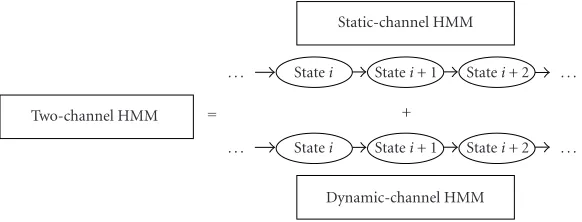
Two-channel HMM = . . .

Static-channel HMM

Statei Statei+ 1 Statei+ 2 . . . +

. . . Statei Statei+ 1 Statei+ 2 . . . Dynamic-channel HMM

Figure1: The block diagram of a two-channel HMM.

This method is referred to as maximum mutual infor-mation (MMI) estiinfor-mation [48]. It increases the a posteriori probability of the model corresponding to the training data, and thus the overall discriminative power of the HMM ob-tained is guaranteed. However, analytical solutions to (2) are difficult to realize and implementation of MMI estimation is tedious. A computationally less intensive approach is desir-able.

3. PRINCIPLES OF TWO-CHANNEL HMM

To improve the discriminative ability of HMM and at the same time, to facilitate the process of parameter tuning, the following two-channel training method is proposed, where the HMM is specially tailored to amplify the difference be-tween two similar samples.

The block diagram of the two-channel HMM is given in

Figure 1. It consists of a static-channel HMM and a dynamic-channel HMM. For the static dynamic-channel, a normal HMM de-rived from a parameter-smoothed ML approach is used. A new HMM for the dynamic channel is to be derived. De-tails of the derivation of the dynamic-channel HMM are de-scribed in the following paragraphs.

Assume that in a two-class identification problem,{xT _: d1} and {yT : d2} are a pair of training samples, where

xT _{= (x}T

1,x2T,. . .,xTT) andyT =(yT1,yT2,. . .,yTT) are

obser-vation sequences of lengthT andd1andd2are the class la-bels. The observed symbols inxT_andyT_{are from the symbol}

setOM_.P(xT_{|θ) andP(y}T_{|θ) are the scored probabilities for} xT _{and y}T _{given HMMθ, respectively. The pair of training}

samplesxT _andyT _{must be of the same length so that their}

probabilitiesP(xT_{|θ) andP(y}T_{|θ) can be suitably compared.}

Such a comparison is meaningless if the samples are of differ-ent lengths; the shorter sequence may give larger probability than the longer one even if it is not the true sample ofθ.

Define a new functionI(xT_,yT_{,θ), called the}

separable-distance function, as follows:

IxT_,yT_,θ=logPxT_|θ−logPyT_{|θ. (3)}

A large value of I(xT_,yT_{,θ) would mean that x}T _and yT _{are more distinct and separable. The strategy then is to}

determine the HMM θMSD (MSD for maximum separable distance) that maximizesI(xT_,yT_{,θ). Mathematically,}

θMSD=arg max

θ

IxT_,yT_{,θ. (4)}

For the proposed training strategy, the parameter set for the static-channel HMM is determined in the normal way such as the ML approach. For the dynamic-channel HMM, to maintain synchronization of the duration and transition of states, the same set of values forπandAas derived for the static-channel HMM is used; only the parameters of matrix

Bare adjusted.

As a first step towards the maximization of the separable-distance function I(xT_,yT_{,θ), an auxiliary}

func-tionF(xT_,yT_{,θ,λ) involvingI(x}T_,yT_{,θ) and the parameters}

ofBis defined as

FxT,yT,θ,λ=IxT,yT,θ+

N

i=1

λi

1− M

j=1

bi j

, (5)

where λi is the Lagrange multiplier for the ith state and

_M

j=1bi j=1 (i=1, 2,. . .,N). By maximizingF(xT,yT,θ,λ), I(xT_,yT_{,θ) is also maximized. DifferentiatingF(x}T_,yT_,θ,λ)

with respect tobi jand setting the result to 0, we have

∂logPxT_|θ ∂bi j −

∂logPyT_|θ

∂bi j =λi. (6)

Since λi is positive, the optimum value obtained for I(xT_,yT_{,θ) is a maximum as solutions forb}

i jmust be

pos-itive. In (6), logP(xT_{|θ) and logP(y}T_{|θ) may be computed}

by summing up all the probabilities over timeT:

logPxT_|θ= T

τ=1 log

N

i=1

PsT τ =Si

bi

xT

τ

. (7)

Note that the state-transition coefficientsai j do not

ap-pear explicitly in (7); they are included in the termP(sT

τ =

The two partial derivatives in (6) may be evaluated sepa-rately as follows:

∂logPxT_|θ ∂bi j =

T

τ=1

xT τ=Oj

PsT

τ =Si|θ,xT

=b−1

i j T

τ=1

PsT

τ =Si,xTτ =Oj|θ,xT

,

∂logPyT_|θ ∂bi j =

T

τ=1

yT τ=Oj

PsT

τ =Si|θ,yT

=b−1

i j T

τ=1

PsT

τ =Si,yTτ =Oj|θ,yT

.

(8)

By defining

ESi,Oj|θ,xT

= T

τ=1

PsT

τ =Si,xτT=Oj|θ,xT

,

ESi,Oj|θ,yT

= T

τ=1

PsT

τ =Si,yTτ =Oj|θ,yT

,

Di j

xT_,yT_,θ=ES

i,Oj|θ,xT

−ESi,Oj|θ,yT

, (9)

equation (6) can be written as

ESi,Oj|θ,xT

−ESi,Oj|θ,yT

bi j

= Di j

xT_,yT_,θ

bi j =λi, 1≤j≤M.

(10)

By making use of the fact thatM_j=1bi j = 1, it can be

shown that

bi j= Di j

xT_,yT_,θ

_M

j=1Di j

xT_,yT_,θ, i=1, 2,. . .,N, j=1, 2,. . .,M.

(11)

The set{bi j}(i = 1, 2,. . .,N, j = 1, 2,. . .,M) so

ob-tained gives the maximum value ofI(xT_,yT_,θ).

An algorithm for the computation of the values may be developed by using standard expectation-maximization (EM) technique. By considering xT _{and y}T _{as the}

ob-served data and the state sequence sT _{= (s}T

1,sT2,. . .,sTT) as

the hidden or unobserved data, the estimation of Eθ(I) = E[I(xT_,yT_,sT_|θ)|xT_,yT_{,θ] from incomplete datax}T _andyT

is then given by [49]

Eθ(I)=

sT_∈S

IxT,yT,sT|θPxT,yT,sT|θ

=

sT_∈S

logPxT_,sT_|θ−logPyT_,sT_|θ

×PxT_,yT_,sT_|θ,

(12)

whereθandθare the HMM before training and the HMM after training, respectively, andSdenotes all the state combi-nations with lengthT. The purpose of the E-step of the EM estimation is to calculateEθ(I). By using the auxiliary

func-tionQx(θ,θ) proposed in [48] and defined as follows:

Qx(θ,θ)=

sT_∈S

logPxT_,sT_|θPxT_,sT_{|θ, (13)}

equation (12) can be written as

Eθ(I)=Qx(θ,θ)P

yT_|sT_,θ−Q y(θ,θ)P

xT_|sT_{,θ. (14)}

Qx(θ,θ) andQy(θ,θ) may be further analyzed by

break-ing up the probabilityP(xT_,sT_{|θ) as follows:}

PxT_,sT_|θ=πs

0

T

τ=1

asτ−1,sτbsτ

xτ

, (15)

whereπ,a, andbare the parameters ofθ. Here, we assume that the initial distribution starts atτ =0 instead ofτ =1 for notational convenience. TheQfunction then becomes

Qx(θ,θ)=

sT_∈S logπs0

PxT_,sT_|θ

+

sT_∈S

_T

τ=1

logaτ−1,τ

PxT_,sT_|θ

+

sT_∈S

_T

τ=1 logbτ

xτ

PxT_,sT_|θ.

(16)

The parameters to be optimized are now separated into three independent terms.

From (14) and (16),Eθ(I) can also be divided into the

following three terms:

Eθ(I)=Eθ(π,I) +Eθ(a,I) +Eθ(b,I), (17)

where

Eθ(π,I)=

sT_∈S logπs0

×PxT_,yT_,sT_|θ−PxT_,yT_,sT_|θ=0,

Eθ(a,I)=

sT_∈S

T

τ=1

logaτ−1,τ

×PxT_,yT_,sT_|θ−PxT_,yT_,sT_|θ=0,

Eθ(b,I)=

sT_∈S

_T

τ=1 logbτ

xτ − T

τ=1 logbτ

yτ

×PxT,yT,sT|θ.

Statei−1 Statei Statei+ 1

[bsi j]

[bdi j]

Weightage=1−ωi Static channel

Weightage=ωi Dynamic channel

Figure2: The two-channel structure of theith state of a left-right HMM.

Eθ(π,I) andEθ(a,I) are associated with the hidden-state

sequencesT_{. It is assumed thatx}T_andyT_{are drawn}

indepen-dently and emitted from the same state sequence sT_{, hence}

both Eθ(π,I) and Eθ(a,I) become 0.Eθ(b,I), on the other

hand, is related to the symbols that appear inxT_andyT_and

contributes toEθ(I). By enumerating all the state

combina-tions, we have

Eθ(b,I)= N

i=1

T

τ=1

logbi

xτT

−logbi

yτT

×PxT,yT,sTτ =Si|θ

.

(19)

IfT_τ=1[logbi(xTτ)−logbi(yτT)] is arranged according to

the order of appearance of the symbols (Oj) withinxT and yT_{, we have}

Eθ(b,I)

= N

i=1

M

j=1 logbi j

T

τ=1

xT τ=yτT=Oj

×PxTτ =Oj,sTτ =Si|θ,xT

−PyτT=Oj,sTτ =Si|θ,yT

×PxT_,yT_|θ

(20)

or

Eθ(b,I)

= N

i=1

M

j=1 logbi j

ESi,Oj|θ,xT

−ESi,Oj|θ,yT

×PxT_,yT_|θ.

(21)

In the M-step of the EM estimation,bi j is adjusted to

maximize Eθ(b,I) or Eθ(I). Since

_M

j=1bi j = 1 and (21)

has the formKMj=1wjlogvj, which attains a global

maxi-mum at the pointvj=wj/

_M

j=1wj(j=1, 2,. . .,M), the

re-estimated value ofbi jofθthat lead to the maximumEθ(I) is

given by

bi j= E

Si,Oj|θ,xT

−ESi,Oj|θ,yT

_M

j=1

ESi,Oj|θ,xT

−ESi,Oj|θ,yT

= Di j

xT_,yT_,θ

_M

j=1Di j

xT_,yT_,θ.

(22)

This equation, compared with (11), enables the re-estimation of the symbol emission coefficientsbi j from

ex-pectations of the existing HMM. The above derivations strictly observe the standard optimization strategy [49], where the expectation of the value of the separable-distance function, Eθ(I), is computed in the E-step and the

coef-ficients bi j are adjusted to maximize Eθ(I) in the M-step.

The convergence of the method is therefore guaranteed. However,bi j may not be estimated by applying (22) alone;

other considerations will be taken into account such as when

Di j(xT,yT,θ) is less than or equal to 0. Further discussion on

the determination of values ofbi jis given in the subsequent

sections.

To modify the parameters according to (22) and simul-taneously ensure the validity of the model, a two-channel structure as depicted inFigure 2is proposed. The elements (bi j) of matrixBof the two-channel HMM are decomposed

into two parts as

bi j=bsi j+bdi j (∀i=1, 2,. . .,N, j=1, 2,. . .,M), (23)

bsi j for the static channel andbi jd for the dynamic channel.

The dynamic-channel coefficientsbd

i j are the key source of

the discriminative power.bsi jare computed using

parameter-smoothed ML HMM and weighted. As long asbi jcomputed

from (22) is greater thanbs

i j,bdi j is determined as the

differ-ence betweenbi j andbsi j according to (23); otherwisebi jd is

set to be 0.

To avoid the occurrence of zero or negative probabil-ity,bi js (∀i=1, 2,. . .,N, ∀j =1, 2,. . .,M) should be kept

the dynamic-channel coefficientbd

i j(∀i=1, 2,. . .,N, ∀j=

1, 2,. . .,M) should be nonnegative. Thus the probability constraintbi j=bsi j+bi jd ≥bsi j>0 is met.

In addition, the relative weightage of the static channel and the dynamic channel may be controlled by the credibility weighing factorωi(i=1, 2,. . .,N) (different states may have

different values). If the weightage of the dynamic channel is set to beωiby scaling of the coefficients

N

j=1

bdi j=ωi, 0≤ωi<1∀i=1, 2,. . .,N, (24)

then the weightage of the static channel has to be set as fol-lows:

N

j=1

bs

i j=1−ωi, 0≤ωi<1∀i=1, 2,. . .,N. (25)

4. TWO-CHANNEL TRAINING STRATEGY

4.1. Parameter initialization

The parameter-smoothed ML HMM of xT_{, θ}x

ML, which is trained using the Baum-Welch estimation, is referred to as the base HMM. The static-channel HMM is derived from the base HMM after applying the scaling factor. Parameter smoothing is carried out forθx

MLto prevent the occurrence of zero probability. Parameter smoothing is the simple man-agement thatbi j is set to some minimum value, for

exam-ple,ε=10−3_{, if the estimated conditional probabilityb}

i j=0

[46]. As a result, even though symbolOjnever appears in the

training set, there is still a nonzero probability of its occur-rence inθxML. Parameter smoothing is a posttraining adjust-ment to decrease error rate because the training set, which is usually limited by its size, may not cover erratic samples.

Before carrying out discriminative training,ωi

(credibil-ity weighing factor of theith state),bsi j(static-channel

coef-ficients), and bdi j (dynamic-channel coefficients) are

initial-ized.

The static-channel coefficientsbi js are given by

bs

i1bsi2· · ·biMs

=1−ωi bi1bi2· · ·biM

, 1≤i≤N, 0≤ωi<1,

(26)

wherebi jis the symbol emission probability ofθMLx . As for the dynamic-channel coefficientsbd

i j, a random or

uniform initial distribution usually works well. In the experi-ments conducted in this paper, uniform values equal toωi/M

are assigned tobdi j’s as initial values.

The selection of ωi is flexible and largely

problem-dependent. A large value ofωimeans large weightage is

as-signed to the dynamic channel and the discriminative power is enhanced. However, as we adjustbd

i j toward the direction

of increasing I(xT_,yT_{,θ), the probability of the correct}

ob-servation P(xT_{|θ) will normally decrease. This situation is}

undesirable because the two-channel HMM obtained is un-likely to generate even the correct samples.

A guideline for the determination of the value ofωiis as

follows. If the training pairs are very similar to each other such thatP(xT_|θx

ML)≈P(yT|θxML),ωishould be set to a large

value to guarantee good discrimination; on the other hand, ifP(xT_|θx

ML)P(yT|θMLx ),ωishould be set to a small value

to makeP(xT_{|θ) reasonably large. In addition, different}

val-ues will be used for different states because they contribute differently to the scored probabilities. However, the values of

ωifor the different states should not differ greatly.

Based on the above considerations, the following proce-dures are taken to determineωi. Given the base HMMθMLx and the training pairxT_andyT_{, the optimal state chains are}

searched using the Viterbi algorithm. If θMLx is a left-right model and the expected (optimal) duration of theith state (i=1, 2,. . .,N) ofxT _{is fromt}

itoti+τi,P(xT|θMLx ) is then written as follows:

PxT|θMLx

=PxTt1,. . .,xt1T+τ1|θxML

Pxt2T,. . .,xTt2+τ2|θMLx

· · ·PxTtN,. . .,x

T tN+τN|θ

x

ML

;

(27)

P(yT_|θx

ML) is decomposed in the same way. LetPdur(xT,Si|θMLx )=P(xTti,. . .,x

T ti+τi|θ

x

ML). This proba-bility may be computed as follows:

Pdur

xT_,S

i|θMLx

= ti+τi

t=ti

_N

j=1

PsT t =Sj

bj

xT

t

. (28)

Pdur(xT,Si|θMLx ) may also be computed using the for-ward variablesαxt(i)=P(xTti+1,. . .,x

T

ti+t,sTti+t=Si|θMLx ) or/and the backward variables βxt(i) = P(xTti+t+1,. . .,xtTi+τi+1|sTti+t =

Si,θMLx ) [46].

However, ifθMLx is not a left-right model but an ergodic model, the expected duration of a state will consist of a num-ber of separated time slices, for example,kslices such asti1 toti1+τi1,ti2toti2+τi2, andtiktotik+τik.Pdur(xT,Si|θxML) is then computed by multiplying them together as shown:

Pdur

xT_,S

i|θMLx

=PxTti1,. . .,x T ti1+τi1|θ

x

ML

PxtTi2,. . .,x T ti2+τi2|θ

x

ML

· · ·PxT tik,. . .,x

T tik+τik|θ

x

ML

.

(29)

The value of ωi is derived by comparing the

corre-sponding Pdur(xT,Si|θxML) and Pdur(yT,Si|θMLx ). IfPdur(xT,

Si|θMLx ) Pdur(yT,Si|θxML), this indicates that the coeffi-cients of the ith state of the base model are good enough for discrimination,ωishould be set to a small value to

pre-serve the original ML configurations. If Pdur(xT,Si|θMLx ) <

Pdur(yT,Si|θxML) orPdur(xT,Si|θxML) ≈Pdur(yT,Si|θMLx ), this indicates that stateSiis not able to distinguish betweenxT

andyT_{, thusω}

HMM. In practice,ωican be manually selected according to

the conditions mentioned above (which is preferred), or they can be computed using the following expression:

ωi= 1

1 +CvD, (30)

wherev=Pdur(xT,Si|θMLx )/Pdur(yT,Si|θMLx ).C(C >0) and

Dare constants that jointly control the smoothness ofωiwith

respect tov. SinceC >0 andv >0,ωi<1, by using suitable

values ofCandD, a set of credibility factorsωiare computed

for the states of the target HMM. For example, if the range of

vis 10−3_∼105_{, a typical setting isC=1.0 andD=0.1.} Once the values ofωi(i = 1, 2,. . .,N) are determined,

they will not be changed in the training process.

4.2. Partition of the observation symbol set

Letθdenote the HMM with the above initial configurations. The coefficients of the dynamic channel are adjusted accord-ing to the followaccord-ing procedures. First, E(Si,Oj|θ,xT) and E(Si,Oj|θ,yT) are computed through the counting process.

Using the forward variablesαx

τ(i)=P(xT1,. . .,xTτ,sTτ =Si|θ)

and backward variables βx

τ(i) = P(xTτ+1,. . .,xTT|sTτ = Si,θ)

[46], the following two probabilities are computed:

ξτx(i,j)=P

sTτ =Si,sτT+1=Sj|xT,θ

= αxτ(i)ai jbj

xTτ+1

βxτ+1(j)

N

i=1

N

j=1αxτ(i)ai jbj

xT τ+1

βx

τ+1(j) ,

γτx(i)=P

sTτ =Si|xT,θ

= N

j=1

ξτx(i,j);

(31)

ξτy(i,j) andγτy(i) are obtained in the same manner. By

count-ing the state, we have

ESi,Oj|θ,xT

= T

τ=1

xT τ=Oj

γx τ(i),

ESi,Oj|θ,yT

= T

τ=1

yT τ=Oj

γτy(i).

(32)

It is shown in (22) that to maximize I(xT_,yT_,θ), bi j should be set proportional to Di j(xT,yT,θ).

How-ever, for certain symbols, for example, Op, the expectation Dip(xT,yT,θ) may be less than 0. Since the symbol

emis-sion coefficients cannot take negative values, these symbols have to be specially treated. For this reason, the symbol set OM _{= {O}

1,O2,. . .,OM} is partitioned into the

sub-set V = {V1,V2,. . .,VK} and its complement set U = {U1,U2,. . .,UM−K}(OM =U∪V) according to the

follow-ing criterion:

V1,V2,. . .,VK

=arg

Oj

ESi,Oj|θ,xT

ESi,Oj|θ,yT > η

(η≥1),

(33)

Symbol label

20 40 60 80 100 120

E

0 5 10 15 20 25

xT yT

(a)

Symbol label

20 40 60 80 100 120

E

0 5 10 15 20 25

xT yT

(b)

Figure3: (a) Distributions ofE(Si,Oj|θ,xT) andE(Si,Oj|θ,yT) for various symbols. (b) Distribution ofE(Si,Oj|θ,xT) for the symbols inV.

whereηis the threshold with a typical value of 1.ηwill be set to a larger value if it is required that the setV will con-tain fewer dominant symbols. Withη≥1,E(Si,Vj|θ,yT)− E(Si,Vj|θ,xT) > 0. As an illustration, the distributions of

the values ofE(Si,Oj|θ,xT) andE(Si,Oj|θ,yT) for different

symbol labels are shown inFigure 3a. The filtered symbols in setVwhenηis set l are shown inFigure 3b.

4.3. Modification to the dynamic channel

For each state, the symbol set is partitioned according to the procedures described inSection 4.2. As an example, consider theith state. For symbols in the setU, the symbol emission coefficientbi(Uj) (Uj∈U) should be set as small as possible.

Letbdi(Uj)=0, and sobi(Uj)=bsi(Uj). For symbols in the

setV, the corresponding dynamic-channel coefficientbd i(Vk)

is computed according to (34), which is derived from (22):

bdi

Vk

=PD

Si,Vk,xT,yT

×

ωi+

K

j=1

bsi

Vj

−bsi

Vk

, k=1, 2,. . .,K,

(34)

where

PD

Si,Vk,xT,yT

= E

Si,Vk|θ,xT

−ESi,Vk|θ,yT

_K

j=1

ESi,Vj|θ,xT

−ESi,Vj|θ,yT

bi2=bsi2

bi1 θt

θt+1

bdi1+bdi2=ωi I=I(xT_,yT_,θ

t+1) I=I(xT_,yT_,θ

t) bil=bsi1

bi2

(a)

bi3=bsi3

bi1 θt θt+1

d d I=I(xT_,yT_,θ

t+1) I=I(xT_,yT_,θt) bil=bsi1

bi3

(b) Figure4: The surface ofIand the direction of parameter adjustment.

However, some coefficients obtained may still be negative, for example,bd

i(Vl)<0 because of large value ofbsi(Vl). In which

case, it indicates thatbs

i(Vl) alone is large enough for

sepa-ration. To prevent negative values appearing in the dynamic channel, the symbolVlis transferred fromVtoUandbdi(Vl)

is set to 0. The coefficients of the remaining symbols inVare reestimated using (34) until allbd

i(Vk)’s are greater than 0.

This situation (somebd

i(Vl)<0) usually happens at the first

few epochs of training and it is not conducive to convergence because there is a steep jump in the surface ofI(xT_,yT_{,θ). To}

relieve this problem, a larger value ofηin (33) will be used.

4.4. Termination

Optimization is done through iteratively calling the training epoch described in Sections 4.2and4.3. After each epoch, the separable-distanceI(xT_,yT_{,θ) of the HMMθobtained,}

is calculated and compared with that obtained in the last epoch. If I(xT_,yT_{,θ) does not change more than a}

prede-fined value, training is terminated and the target two-channel HMM is established.

5. PROPERTIES OF THE TWO-CHANNEL TRAINING STRATEGY

5.1. State alignment

One of the requirements for the proposed training strategy is that the state durations of the training pair, say xT _and yT_{, are comparable. This is a requirement for (22). If the}

state durations, for example,E(Si|θ,xT) andE(Si|θ,yT),

dif-fer too much, Di j(xT,yT,θ) will become meaningless. For

example, ifE(Si|θ,xT) E(Si|θ,yT), the symbolOj takes

much greater portion inE(Si|θ,xT) than inE(Si|θ,yT), the

computedDi j(xT,yT,θ) may also be less than 0. The

out-come is thatbi j is always set tobsi j rather than adjusted to

increaseI(xT_,yT_{,θ). Fortunately, if the corresponding state}

durations of the training pair are very different, the normal ML HMMs are usually adequate to distinguish the states.

The following state-duration validation procedure is added to make the training strategy complete. After each training epoch,E(Si|θ,xT) andE(Si|θ,yT) are computed and

compared with each other. Using the forward variables and backward variables, the state duration of xT _{is obtained as}

follows:

ESi|θ,xT

= T

τ=1

αx τ(i)βxτ(i)

_N

i=1αxτ(i)βτx(i)

, i=1, 2,. . .,N, (36)

andE(Si|θ,yT) is computed in the same way. IfE(Si|θ,xT)≈ E(Si|θ,yT) (not necessary to be the same), for example,

1.2E(Si|θ,yT)> E(Si|θ,xT) > 0.8E(Si|θ,yT), training

con-tinues; otherwise, training stops even ifI(xT_,yT_{,θ) keeps on}

increasing.

If theI(xT_,yT_{,θ) of the final HMMθdoes not meet}

cer-tain discriminative requirement, for example,I(xT_,yT_{,θ) is}

less than a desired value, a new base HMM or a smaller ωi

should be used instead.

5.2. Speed of convergence

As discussed inSection 3, the convergence of the parameter-estimation strategy proposed in (22) is guaranteed accord-ing to the EM optimization principles. In the implemen-tation of discriminative training, only some of the symbol emission coefficients in the dynamic channel are modified according to (22) while the others remain unchanged. How-ever, the convergence is still assured because firstly the surface ofI(xT_,yT_{,θ) with respect tob}

i jis continuous, and also

ad-justing the dynamic-channel elements according to the two-channel training strategy leads to increasedEθ(I). A

concep-tual illustration is given inFigure 4on howbi j is modified

for stateSi. Letθtdenote the HMM trained at thetth round

and letθt+1denote the HMM obtained at thet+ 1th round. The surface of the separable distance (I surface) is denoted asI = I(xT_,yT_,θ

t+1) forθt+1 andI = I(xT,yT,θt) forθt.

ClearlyI > I. TheI surface is mapped to thebi1-bi2plane (Figure 4a) and thebi1-bi3plane (Figure 4b). In the training phase,bi1andbi2are modified along the linebid1+bdi2=ωito

reach a better estimationθt+1, which is shown inFigure 4a. In thebi1-bi3plane,bi3is set to the constantbsi3whilebi1is mod-ified along the linebi3 = bsi3with the direction

das shown in Figure 4b. The direction of parameter adjustment given by (22) is denoted byd. In the two-channel approach, since onlybi1andbi2are modified according to (22) whilebi3 re-mains unchanged,_dmay lead to lower speed of convergence thanddoes.

5.3. Improvement to the discriminative power

The improvement to the discriminative power is estimated as follows. Assume thatθ is the two-channel HMM obtained. The lower bound of the probabilityP(yT_{|θ) is given by}

PyT|θ≥1−ωmax

T

PyT|θMLx

, (37)

whereωmax=max(ω1,ω2,. . .,ωN).

Because the base HMM is the parameter-smoothed ML HMM of xT_{, it is natural to assume that P(x}T_|θx

ML) ≥

P(xT_{|θ). The upper bound of the separable distance is given}

by the following expression:

IxT_,yT_,θ≤log P

xT_|θx

ML

1−ωmax

T

PyT_|θx

ML

= −Tlog1−ωmax

+IxT_,yT_,θx

ML

.

(38)

In practice, the gain ofI(xT_,yT_{,θ) is much smaller than}

the theoretical upper bound. It depends on the resemblance betweenxT_andyT_{, and the setting ofω}

i.

6. EXTENSIONS OF THE TWO-CHANNEL TRAINING ALGORITHM

6.1. Training samples with different lengths

Up to this point, the training sequences are assumed to be of equal length. This is necessary as we cannot properly compare the probability scores of two sequences of different lengths. To extend the training strategy to sequences of differ-ent lengths, linear adjustmdiffer-ent is first carried out as follows. Given the training pairxTx_{of lengthTxandy}Ty_{of lengthTy,}

the objective function (10) is modified as follows:

λi=

Tx

τ=1P

sTx

τ =Si,xTτx=Oj|θ,xTx

bi j

−

Tx/Ty Tτ=y1P

sTy

τ =Si,yτTy =Oj|θ,yTy

bi j

∀j=1, 2. . .,M.

(39)

Parameter estimation is then carried out as follows:

bi j= E

Si,Oj|θ,xTx

−Tx/Ty

ESi,Oj|θ,yTy

_M

j=1

ESi,Oj|θ,xTx−T_x/T_yES_i,O_j|θ,yTy. (40)

The expectations of different states of yTy _are normal-ized using the scale factor Tx/Ty. This approach is easy to

implement; however, it does not consider the nonlinear vari-ance of signal such as local stretch or squash. If the train-ing sequences demonstrate obvious nonlinear variance, some nonlinear processing such as sequence truncation or symbol prune may be carried out to adjust the training sequences to the same length [50].

6.2. Multiple training samples

In order to obtain a reliable model, multiple observations must be used to train the HMM. The extension of the pro-posed method to include multiple training samples may be carried out as follows. Consider two labeled sets X = {x(1)_,x(2)_{,. . .,x}(k) _{: d}

1} andY = {y(1),y(2),. . .,y(l) : d2} of samples, where X has k number of samples andY has

l number of samples. The separable-distance function that takes care of all these samples is given by

I(X,Y,θ)=1 k

k

m=1

logPx(m)|θ−1 l

k

n=1

logPy(n)|θ.

(41)

For simplicity, if we assume that the observation se-quences inXandY have the same lengthT, then (10) may be rewritten as

(1/k)k_m=1E

Si,Oj|θ,x(m)

−(1/l)l_n=1E

Si,Oj|θ,y(n)

bi j =λi, 1≤j≤M.

(42)

The probability coefficients are then estimated using the following:

bi j=

(1/k)k_m=1E

Si,Oj|θ,x(m)

−(1/l)l_n=1E

Si,Oj|θ,y(n)

_M

j=1

(1/k)k_m=1E

Si,Oj|θ,x(m)

−(1/l)l_n=1E

Si,Oj|θ,y(n)

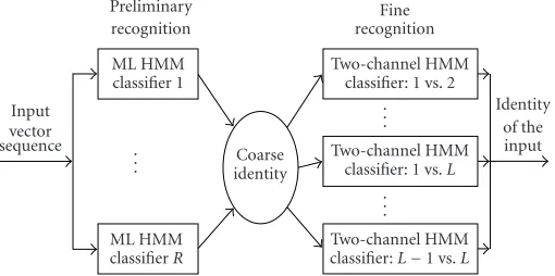
ML HMM classifierR

. . . ML HMM classifier 1 Preliminary recognition

Two-channel HMM classifier:L−1 vs.L

. . .

Two-channel HMM classifier: 1 vs.L

. . .

Two-channel HMM classifier: 1 vs. 2

Fine recognition

Coarse identity Input

vector sequence

Identity of the input

Figure5: Block diagram of the viseme recognition system.

Table1: The 18 visemes selected for the experiments.

/a:/, /ai/, /æ/, /ei/, /i/, /j/, /ie/, /o/, /oi/, /th/, /sh/, /tZ/, /dZ/, /eu/, /au/, /p/, /m/, /b/

7. APPLICATION TO LIP READING

The proposed two-channel HMM method is applied to speaker-dependent lip reading for modeling and recogniz-ing the basic visual speech elements of the English language. For the experiments reported in this paper, the visemes are treated as having a one-to-one mapping with the phonemes in order to test the discriminative power of the proposed method. As there are 48 phonemes in the English language [47], 48 visemes are considered.

The block diagram of the viseme recognition system is given inFigure 5. The lip movement is captured with a video camera and the sequence of images is processed to extract the essential features relevant to the lip movement. For each frame of image, a feature vector is extracted. The sequence of feature vectors thus represents the movement of lips during viseme production. This vector sequence is then presented as input to the proposed classifier. A hierarchical structure is adopted such that for a system withKvisemes to be recog-nized,R(usuallyR < K) ML HMM classifiers are employed for preliminary recognition. The output of the preliminary recognition is a coarse identity, which may includeL (usu-ally 1< L < K) viseme classes. Fine recognition is then per-formed using a bank of two-channel HMMs. The most prob-able viseme is then chosen as the identity of the input. Details of the various steps involved are given in the following sec-tions.

7.1. Data acquisition

For our experiments, a professional English speaker is en-gaged. The speaker is asked to articulate every phone me of the 18 phonemes inTable 1 one hundred times. The 18 visemes are chosen as some of them bear close similarity to others. The lip movements of the speakers are captured at 50 frames per second. Each pronunciation starts from a closed mouth and ends with a closed mouth. This type of samples is

referred to as text-independent viseme samples, which is dif-ferent from the type of samples extracted from various con-texts, for example, from different words. The video clips that indicate the productions of context-independent visemes are normalized such that all the visemes have uniform duration of 0.5 second, or equivalently 25 frames.

7.2. Feature extraction

Each frame of the video clip reveals the lip area of the speaker during articulation (Figure 6a). To eliminate the ef-fect caused by changes in the brightness, the RGB (red, green, blue) factors of the image are converted into HSV (hue, sat-uration, value) factors. The RGB to HSV conversion algo-rithm proposed in [51,52] is adopted in our experiments. As illustrated in the histograms of distribution of the hue com-ponent shown inFigure 7, the hue factors of the lip region and the remaining lip-excluded image occupy different re-gions of the histogram. A threshold may be manually selected to segment the lip region from the entire image as shown in

Figure 6b. This threshold usually corresponds to a local min-imum point (valley) in the histogram as shown inFigure 7a. Note that for different speakers and lighting conditions, the threshold may be different.

50 100 150 140

120 100 80 60 40 20

(a)

50 100 150 140

120 100 80 60 40 20

(b)

R1

R2 R3

C1

C2 C3

(c)

1

2

3

4 5 6 7

8 9

10 11

(d)

Figure6: (a) Original image. (b) Segmented lip area. (c) Parameterized lip template. (d) Geometric measures extracted from the lip template. (1) Thickness of the upper bow. (2) Thickness of the lower bow. (3) Thickness of the lip corner. (4) Position of the lip corner. (5) Position of the upper lip. (6) Position of the lower bow. (7) Curvature of the upper-exterior boundary. (8) Curvature of the lower-exterior boundary. (9) Curvature of the upper-interior boundary. (10) Curvature of the lower-interior boundary. (11) Width of the tongue (when it is visible).

following four terms:

Elip= −1

R1

R1H(x)dx,

Eedge= − 1

C1+C2

C1+C2

_H+_(x)−H(x)

+H−(x)−H(x)dx,

Ehole= − 1

R2−R3

R2−R3H(x)dx, Einertia=Γt+1−Γt

2 ,

(44)

whereR1,R2,R3,C1, andC2are areas and contours as illus-trated inFigure 6c.H(x) is a function of the hue of a given pixel;H+_{(x) is the hue function of the closest right-hand side} pixel and H−(x) is that of the closest left-hand side pixel.

Γt+1 andΓt are the matched templates at timet+ 1 and t. Γt+1−Γtindicates the Euclidean distance between the two

templates (further details may be found in [55]). The over-all energy of the templateEis the linear combination of the components defined as

E=c1Elip+c2Eedge+c3Ehole+c4Einertia. (45)

Similarly, the energy terms for the tongue template in-clude

Etongue-area= − 1

R3

R3H(x)dx ifR3>0,

Etongue-edge= − 1

C3

C3

_H+_(x)−H(x)

+H−(x)−H(x)dx ifC3>0,

Etongue-inertia=Ttongue,t+1−Ttongue,t2,

(46)

and the overall energy is

Etongue=c5Etongue-area+c6Etongue-edge+c7Etongue-inertia. (47)

Initially, the dynamic contours are configured to provide a crude match to the lips. This can be done via comparing the enclosed region of the template and the segmented lip re-gion as depicted inFigure 6b. Following that, the template is matched to the image sequence by adopting different values of the parameters{ci}(i=1, 2,. . ., 7) in a number of

search-ing epochs (a detailed discussion is given in [53,54,55]). The matched template is pictured inFigure 6d. It can be seen that the matched template is symmetric and smooth, and is there-fore easy to process.

Eleven geometric parameters as shown inFigure 6dare extracted to form a feature vector from the matched tem-plate. These features indicate the thickness of various parts of the lips, the positions of some key points, and the curvatures of the bows. They are chosen as they uniquely determine the shape of the lips and they best characterize the movement of the lips.

Principal components analysis (PCA) is carried out to reduce the dimension of the feature vectors from eleven to seven. The resulting feature vectors are clustered into groups usingK-means algorithm. In the experiments con-ducted, 128 clusters are created for the vector database. The means of the 128 clusters form the symbol set O128 ₌ (O1,O2,. . .,O128) of the HMM. They are used to encode the vector sequences presented to the system.

7.3. Configuration of the viseme model

Investigation on the lip dynamics reveals that the movement of the lips can be partitioned into three phases during the production of a text-independent viseme. The initial phase begins with a closed mouth and ends with the start of sound production. The intermediate phase is the articulation phase, which is the period when sound is produced. The third phase is the end phase when the mouth restores to the relaxed state.Figure 8illustrates the change of the lips in the three phases and the corresponding acoustic waveform when the phoneme /u/ is uttered.

0 0.2 0.4 0.6 0.8 1 0

50 100 150 200 250 300 350 400 450

Threshold

(a)

0 0.2 0.4 0.6 0.8 1

0 50 100 150 200 250 300 350 400

(b)

0 0.2 0.4 0.6 0.8 1

0 50 100 150 200 250 300 350 400 450

(c)

Figure7: Isolation of the lip region from the entire image using hue distribution. (a) Histogram of the hue component for the entire image. (b) Histogram of the hue component for the actual lip region. (c) Histogram of the hue component for the actual lip-excluded image.

Using this structure, the state-transition matrixAhas the form

A=

    

a1,1 a1,2 0 0 0 a2,2 a2,3 0 0 0 a3,3 a3,4

0 0 0 1

   

, (48)

where the 4th state is a null state that indicates the end of viseme production. The initial values of the coefficients in matrices A andB are set according to the statistics of the three phases. Given a viseme sample, the approximate ini-tial phase, articulation phase, and end phase are segmented from the image sequence and the acoustic signal (an illus-tration is given inFigure 8), and the duration of each phase

is counted. The coefficientsai,iandai,i+1are initialized with these durations. For example, if the duration of stateSiisTi,

the initial value ofai,iis set to beTi/(Ti+ 1) and the initial

value ofai,i+1is set to be 1/(Ti+ 1) as they maximizeaTi,iiai,i+1. MatrixBis initialized in a similar manner. If symbolOj

ap-pearsT(Oj) times in stateSi, the initial value ofbi jis set to

beT(Oj)/Ti. For such arrangement, the states of the HMM

are aligned with the three phases of viseme production and hence are referred to as the initial state, articulation state, and end state.

0 500 1000 1500 2000 2500 3000 3500 4000 −2

−1 0 1 2

(a) (b) (c)

1 2 3

· · · · · ·

Figure8: The three phases of viseme production. (a) Initial phase. (b) Articulation phase. (c) End phase.

Initial Articulation End

Figure9: Three-state left-right viseme model.

7.4. Viseme classifier

The block diagram of the proposed hierarchical viseme clas-sifier is given inFigure 10. For visemes that are too similar to be separated by the normal ML HMMs, they are clustered into one macro class. In the figure,θMac1,θMac2,. . .,θMacRare

the Rnumber of ML HMMs for theRmacro classes. The similarity between the visemes is measured as follows.

Assume thatXi= {xi1,x2i,. . .,xili :di}is the training sam-ples of visemedi(i=1, 2,. . ., 18, as 18 visemes are involved),

wherexi

jis thejth training sample andliis the number of the

samples. An ML HMM is trained for each of the 18 visemes using the Baum-Welch estimation. Letθ1,θ2,. . .,θ18denote the 18 ML HMMs. For{xi1,xi2,. . .,xlii :di}, the joint proba-bility scored byθjis computed as follows:

PXi|θj

= li

n=1

Pxni|θj

. (49)

A viseme modelθiis able to separate visemesdianddjif

the following condition applies:

logPXi|θi

−logPXi|θj

≥Kli ∀j=1, 2,. . ., 18, j=i,

(50)

where K is a positive constant that is set according to the length of the training samples. For long training samples, a large value ofKis desired. For the 25-length samples adopted in our experiments,Kis set to be equal to 2. If the condition stated in (50) is not met, visemesdianddj are categorized

into the same macro class. The training samples ofdianddj

are jointly used to train the ML HMM of the macro class.

θMac1,θMac2,. . .,θMacRare obtained in this way.

For an input visemezT_{to be identified, the probabilities} P(zT_|θ

Mac1),P(zT|θMac2),. . .,P(zT|θMacR) are computed and

compared with one another. The macro identity ofzT _is

de-termined by the HMM that gives the largest probability.

A macro class may consist of several similar visemes. Fine recognition within a macro class is carried out at the sec-ond layer. Assume that Macro ClassicomprisesLvisemes:

V1,V2,. . .,VL. A number of two-channel HMMs are trained

with the proposed discriminative training strategy. ForV1,

L−1HMMs,θ1∧2,θ1∧3,. . .,θ1∧L, are trained to separate the

samples ofV1from those ofV2,V3,. . .,VL, respectively. Take θ1∧2 as an example, the parameter-smoothed ML HMM of

V1,θ1ML, is adopted as the base HMM. The samples ofV1are used as the correct samples (xT _{in (3)) and the samples of} V2are used as the incorrect samples (yT in (3)) while train-ingθ1∧2. There is a total ofL(L−1) two-channel HMMs in Macro Classi.

For an input visemezT_{to be identified, the following}

hy-pothesis is made:

Hi∧j=     

i if logPzT_|θ i∧j

−logPzT_|θ j∧i

> K,

0 otherwise, (51)

whereK is the positive constant as defined in (47). For the 25-frame sequence input to the system, K is chosen to be equal to 2. Hi∧j = i indicates a vote forVi. The decision

about the identity ofzT _{is made by a majority vote of all the}

two-channel HMMs. The viseme class that has the maximum number of votes is chosen as the identity ofzT_{, denoted by}

ID(zT_{). Mathematically,}

IDzT_=max i

Number ofHi∧j=i

∀i,j=1, 2,. . .,L,i=j.

(52)

If two viseme classes, say Vi and Vj, receive the same