Joint Source-Channel Decoding of Variable-Length
Codes with Soft Information: A Survey
Christine Guillemot
IRISA-INRIA, Campus de Beaulieu, 35042 Rennes Cedex, France Email:[email protected]
Pierre Siohan
R&D Division, France Telecom, 35512 Rennes Cedex, France Email:[email protected]
Received 13 October 2003; Revised 27 August 2004
Multimedia transmission over time-varying wireless channels presents a number of challenges beyond existing capabilities con-ceived so far for third-generation networks. Efficient quality-of-service (QoS) provisioning for multimedia on these channels may in particular require a loosening and a rethinking of the layer separation principle. In that context, joint source-channel decod-ing (JSCD) strategies have gained attention as viable alternatives to separate decoddecod-ing of source and channel codes. A statistical framework based on hidden Markov models (HMMs) capturing dependencies between the source and channel coding compo-nents sets the foundation for optimal design of techniques of joint decoding of source and channel codes. The problem has been largely addressed in the research community, by considering both fixed-length codes (FLC) and variable-length source codes (VLC) widely used in compression standards. Joint source-channel decoding of VLC raises specific difficulties due to the fact that the segmentation of the received bitstream into source symbols is random. This paper makes a survey of recent theoretical and practical advances in the area of JSCD with soft information of VLC-encoded sources. It first describes the main paths followed for designing efficient estimators for VLC-encoded sources, the key component of the JSCD iterative structure. It then presents the main issues involved in the application of the turbo principle to JSCD of VLC-encoded sources as well as the main approaches to source-controlled channel decoding. This survey terminates by performance illustrations with real image and video decoding systems.
Keywords and phrases:joint source-channel decoding, source-controlled decoding, turbo principle, variable-length codes.
1. INTRODUCTION
The advent of wireless communications, ultimately in a global mobility context with highly varying channel char-acteristics, is creating challenging problems in the area of coding. Design principles prevailing so far and stemming from Shannon’s source and channel separation theorem are being reconsidered. The separation theorem, stating that source and channel optimum performance bounds can be approached as close as desired by designing independently source and channel coding strategies, holds only under asymptotic conditions where both codes are allowed infinite length and complexity, and under conditions of source sta-tionarity. If the design of the system is heavily constrained in terms of complexity or delay, source and channel coders can be largely suboptimal, leading to residual channel error rates, which can be large and lead to dramatic source symbol error rates. The assumption prevailing so far was essentially that the lower layers would offer a guaranteed delivery
ser-vice, with a null residual bit error rate: for example, the error detection mechanism supported by the user datagram proto-col (UDP) discards all UDP packets corrupted by bit errors, even if those errors are occurring in the packet payload. The specification of a version of UDP, called UDP-Lite [1], that would allow to pass erroneous data to the application layer (i.e., to the source decoder) to make the best use of error-resilient decoding systems is under study within the Internet Engineering Task Force (IETF).
at decorrelating the signal followed by a channel coder that aims at reaugmenting the redundancy in the transmitted stream in order to cope with transmission errors. The key idea of JSCD is to exploit jointly the residual redundancy of the source-coded stream (i.e., exploiting the sub-optimality of the source coder) and the redundancy introduced by the channel code in order to correct bit errors, and find the best source-symbols estimates.
Early work reported in the literature assumed fixed-length representations (FLC) for the quantized-source in-dexes [7,8,9,10]. Correlation between successive indexes in a Markovian framework is exploited to find maximum a posteriori (MAP) or minimum mean square error (MMSE) estimates. The applications targeted by research on error-resilient FLC decoding and JSCD of FLC are essentially speech applications making use for instance of CELP codecs. However, the wide use of VLC in data compression, in partic-ular for compressing images and video signals, has motivated more recent consideration of variable-length coded streams. As in the case of FLC, VLC decoding with soft information amounts to capitalize on source coder suboptimality, by ex-ploiting residual source redundancy (the so-called “excess-rate”) [11,12,13,14,15]. However, VLC decoding raises extra difficulties resulting from the lack of synchronization between the symbol and bit instants in presence of bit er-rors. In other words, the position of the symbol boundaries in the sequence of noisy bits (or measurements) is not known with certainty. This position is indeed a random variable, the value of which depends on the realization of all the previous symbols in the sequence. Hence, the segmentation of the bit-stream into codewords is random, which is not the case for FLCs. The problem becomes a joint problem of segmentation and estimation which is best solved by exploiting both inter-symbol correlation (when the source is not white) as well as inner-codeword redundancy resulting from the entropy code suboptimality.
This problem has first been addressed by considering tree-based codes such as Huffman codes [11, 16, 17]. In this case, the entropy-coded bitstream can be modelled as a semi-Markov process, that is, as a function of a hidden Markov process. The resulting dependency structures are well adapted for MAP (maximum a posteriori) and MPM (maximum of posterior marginals) estimation, making use of soft-input soft-output dynamic decoding algorithms such as the soft-output Viterbi algorithm (SOVA) [18] or the BCJR algorithm [19]. To solve this problem, various trel-lis representations have been proposed, either assuming the source to be i.i.d. as in [20,21], or also taking into account the intersymbol dependencies. In source coding, the mean square error (MSE) being a privileged performance measure, a conditional mean or MMSE criterion can also be used, possibly with approximations to maintain the computational complexity within a tractable range [22].
The introduction of arithmetic codes in practical systems (e.g., JPEG-2000, H.264) has then moved the effort towards the design of robust decoding techniques of arithmetic codes. Sequential decoding of arithmetic codes is investigated in [23] for supporting error correction capabilities. Sequential
decoding with soft output and different paths pruning tech-niques are described in [24,25]. Additional error detection and correction capabilities are obtained in [26] by reintro-ducing redundancy in the form of parity-check bits embed-ded in the arithmetic coding procedure. A probability inter-val not assigned to a symbol of the source alphabet or mark-ers inserted at known positions in the sequence of symbols to be encoded is exploited for error detection in [27,28,29]. The authors in [30] consider quasiarithmetic codes which, in contrast with optimal arithmetic codes, can be modelled as finite-state automata (FSA).
When an error-correcting code (ECC) is present in the communication chain, optimum decoding can be achieved by making joint use of both forms of redundancy: the source “excess-rate” and the redundancy introduced by the ECC. This is the key idea underlying all joint source-channel de-coding strategies. Joint use of correlation between quantized indexes (i.e., using fixed-length representations of the in-dexes) and of redundancy introduced by a channel turbo coder is proposed in [31]. The approach combines the Markovian source model with a parallel turbo coder model in a product model. In order to reduce the complexity, an it-erative structure, in the spirit of serial turbo codes where the source coder is separated from the channel coder by an in-terleaver, is described in [32]. The convergence behavior of iterative source-channel decoding with fixed-length source codes and a serial structure is studied in [33] using EXIT charts [34]. The gain brought by the iterations is obviously very much dependent on the amount of correlation present on both sides of the interleaver.
Models incorporating both VLC-encoded sources and channel codes have been considered in [16,17,35,36]. The authors in [16] derive a global stochastic automaton model of the transmitted bitstream by computing the product of the separate models for the Markov source, the source coder, and the channel coder. The resulting automaton is used to per-form a MAP decoding with the Viterbi algorithm. The ap-proach provides optimal joint decoding of the chain, but re-mains untractable for realistic applications because of state explosion. In [35,36,37], the authors remove the memory assumption for the source. They propose a turbo-like itera-tive decoder for estimating the transmitted symbol stream, which alternates channel decoding and VLC decoding. This solution has the advantage of using one model at a time, thus avoiding the state explosion phenomenon. The authors in [14] push further the above idea by designing an iterative es-timation technique alternating the use of the three models (Markov source, source coder, and channel coder). A parallel iterative joint source-channel decoding structure is also pro-posed in [38].
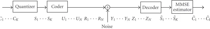
Quantizer Coder + Decoder estimatorMMSE C1· · ·CK S1· · ·SK U1· · ·UN R1· · ·RN Y1· · ·YNZ1· · ·ZN S1· · ·SK C1· · ·CK
Noise
Figure1: Overview of the source-channel coding chain.
cover the case of VLC used in conjunction with convolutional and turbo codes [42,43].
The rest of the paper is organized as follows.Section 2 describes part of the notations used and briefly revisits es-timation criteria (MAP, MPM, MMSE) and algorithms on which we rely in the sequel. Section 3 presents models of dependencies and corresponding graph representations for source coders which can be modelled as FSA. Estimation us-ing trellis decodus-ing algorithms can be run on the resultus-ing dependency graphs. When the coder cannot be modelled as a finite-state automaton, sequential decoding with soft out-put can be applied as explained inSection 3.5. The problem of complexity resulting from large state-space dimensions for realistic sources is addressed inSection 3.6where the graph of dependencies of the source coder is separated into two separate graphs exchanging information along a dependency tree-structure. Mechanisms to improve the decoder’s resyn-chronization capability are described inSection 4.Section 5 presents joint source-channel decoding principles placing the above material in an iterative decoding structure in the spirit of serial and parallel turbo codes. Section 6gives an overview of channel decoding with the help of a priori source information. InSection 7, we present the estimation prob-lem of the source statistics from noisy information. Finally, Section 8, in light of performance illustrations with real im-age and video coding/decoding systems, discusses the poten-tial of JSCD strategies.
2. BACKGROUND
In order to introduce the notations and the background of estimation techniques, we first consider the simple coding and transmission chain depicted inFigure 1. We reserve cap-ital letters to random variables, and small letters to values of these variables. LetCK1 =C1· · ·CK be a sequence of source symbols to be quantized and coded and letSK1 =S1· · ·SK be the corresponding sequence of quantized symbols tak-ing their values in a finite alphabetAcomposed ofQ=2q symbols,A= {a1,a2,. . .,ai,. . .,aQ}. The sequenceSis then
coded into a sequence of bitsU1N =U1· · ·UN, by means of a coder, that can encompass a source or/and a channel coder as we will see later.
The lengthNof the useful bitstream is a random variable, a function ofSK1 and of the coding processes involved in the
chain. However, in most transmission systems, the encoded version ofSK1 is delimited by a prefix and a suffix that allow
a reliable isolation of U1N. Therefore, one can assume that
Nis perfectly observed. A sequence of redundant bitsRN1 =
R1· · ·RNmay be added toU1Nby means of a correcting code
(Figure 1and the notationRN1 correspond to the case where
a systematic rate 1/2 code is used).
The bitstream U1N is sent over a memoryless channel and received as measurementsY1N (seeFigure 1). LetY1N =
Y1· · ·YN be pointwise (noisy) measurements on the se-quence of bitsU1N. The sequenceY1N models the output of
the discrete channel, the quantities yN1 = y1· · ·yN denot-ing the particular values ofY1Nobserved at the output of the channel. The decoding problem consists in finding an esti-mateSK1 of the sequenceSK1, and ultimately reconstructing
CK
1, given the observed values yN1 on the useful bits andz1N
on the redundant bits.
Assuming thatCK1 andSK1 are standard Markov processes, the problem becomes a classical hidden Markov inference problem for which efficient algorithms, known under a va-riety of names (e.g., Kalman smoother, Raugh-Tung-Striebel algorithm, BCJR algorithm, belief propagation, sum-product algorithm, etc.), exist. The problem is indeed to estimate the sequence of hidden states of a Markovian source through observations of the output of a memoryless channel. The estimation algorithms often differ by the estimation crite-ria (MAP, maximum likelihood (ML), MPM, and minimum mean square error (MMSE)) and the way the computations are organized. The decision rules can be either optimum with respect to a sequence of symbols or with respect to individual symbols.
2.1. MAP estimates (or “sequence” MAP decoding) The MAP estimate of the whole processSK1 based on all
avail-able measurementsY1Ncan be expressed as1
SK
1 =S1· · ·SK=arg max s1···sKP
s1· · ·sK|y1· · ·yN
. (1)
The optimization is thus made over all possible sequences realizations sK1 of bit length N. Assuming that the sym-bolsSk are converted into a fixed number of bits (using a FLC), when the a priori information is equally distributed, it can be shown easily that, using the Bayes formula, the “se-quence” MAP (P(SK1|Y1N)) is equivalent to the ML estimate
(P(Y1N|SK1)). The ML estimate can be computed with the
Viterbi algorithm (VA). When the a priori information is not equally distributed, the “sequence” MAP can still be derived from the ML estimate, as a subproduct of the VA, if the met-ric incorporates the a priori probabilitiesP(Sk+1|Sk). If the
1For notational convenience, in the sections where a channel coder is
symbolsSkare converted into variable numbers of bits, one has to use instead the generalized Viterbi algorithm [44].
In ML and MAP estimations, the ratios of probabili-ties of trellis paths leading to a given stateX to the sum of probabilities of all possible paths terminated atX are often computed as likelihood ratiosor in the logarithmic domain as log-likelihood ratios (LLRs). Modifications have been in-troduced in the VA in order to obtain at the decoder output, in addition to the “hard”-decoded symbols, reliability infor-mation, leading to the soft-output Viterbi algorithm (SOVA) [18]. The ML or sequence MAP estimation algorithms do supply sequence a posteriori probabilities but not actual a posteriori symbol probabilities, hence are not optimal in the sense of symbol error probability.
2.2. MPM estimation (or “symbol-by-symbol” MAP decoding)
The symbol-by-symbol MAP decoding algorithms search for the MPM estimates, that is, estimate each hidden state of the Markov chain individually according to
Sk=arg maxs
k P
Sk=sk|Y1N =y1N
. (2)
Assuming that the symbols Sk are converted into a fixed number of bits (using a FLC), computations can be orga-nized around the factorization
PSk|YN 1
∝PSk,Y1n
·PYN n+1|Sk
, (3)
where∝denotes a renormalization. The measuresYnon bits
Uncan indeed be converted into measures on symbols in a very straightforward manner. In the case of VLC encoding of the symbolsSk, the conversion brings some slight technical difficulty (we return to this point inSection 3).
First “symbol-by-symbol” MAP decoding algorithms have been known from the late sixties [45], early seventies [19,46]. The Markov property allows a recursive computa-tion of both terms of the right-hand side organized in a for-ward and backfor-ward recursion. The BCJR algorithm is a two-recursion algorithm involving soft decisions and estimating per-symbol a posteriori probabilities. To reconstruct the data sequence, the soft output of the BCJR algorithm are hard lim-ited. The estimates need not form a connected path in the estimation trellis.
Because of its complexity, the implementation of the MAP estimation has been proposed in the logarithmic do-main leading to a log-MAP algorithm [47,48]. In its log-arithmic form, exponentials related to the classical additive white Gaussian noise (AWGN) channel disappear, and mul-tiplications become additions. Further simplifications and approximations to the log-MAP algorithm have been pro-posed in order to avoid calculating the actual probabili-ties. These simplifications consist in replacing the additions by some sort of MAX operations plus a logarithmic term (ln(1 + exp(−|a−b|))). Ignoring the logarithmic term leads to the suboptimal variant known as the Max-Log-MAP algo-rithm [48].
2.3. MMSE decoding
The performance measure of source coding-decoding sys-tems is traditionally the MSE between the reconstructed and the original signal. In that case, the MAP criterion is sub-optimal. Optimal decoding is given instead by conditional mean or MMSE estimators. The decoder seeks the sequence of reconstruction values (a1· · ·ak· · ·aK), ak ∈ R, k = 1,. . .,K, for the sequence C1K. The values ak may not be-long to the alphabet used initially to quantize the sequence of symbolsC1K. This sequence of reconstruction values should
be such that the expected distortion on the reconstructed se-quenceCK1, given the sequence of observationsY1N, and
de-noted byE[D(CK1,C1K)|Y1N], is minimized. This expected
dis-tortion can be computed from the a posteriori probabilities (APPs) of the estimated quantized sequenceSK1, given the se-quence of measurements, obtained as a result of the sese-quence MAP estimation described above.
However, minimizing E[D(C1K,CK1)|Y1N], that is, given
the entire sequence of measurements, becomes rapidly untractable except in trivial cases. Approximate solutions (approximate MMSE estimators (AMMSE)) considering the expected distortion for each reconstructed symbol
E[D(Ck,Ck)|YN
1] are used instead [22]. The problem then
amounts to minimizing
D=K k=1
M
l=1
al−ak2
PSk=al|Y1N =y1N
, (4)
whereMis the size of the reconstruction alphabet, and the reconstruction valuesakare centroids computed as
ak= M
l=1
alPSk=al|Y1N =yN1
. (5)
The termP[Sk =al| Y1N = y1N] turns out to be the
poste-rior marginals computed with the MPM strategy described above, that is, with the forward/backward recursion as in [19].
3. SOFT-INPUT SOFT-OUTPUT SOURCE DECODING
The application of the turbo principle to JSCD, according to serial or parallel structures, as we will see in Section 5, re-quires first to design soft-input soft-output source decoding algorithm. The problem is, given the sequence of observa-tionsY1N (sequence of noisy bits received by the source de-coder), to estimate the sequence of symbols SK1. The term
“soft” here means that the decoder takes in input, and sup-plies, not only binary (“hard”) decisions, but also a mea-sure of confidence (i.e., a probability) on the bits. The de-pendencies between the quantized indexes are assumed to be Markovian, that is, the sequence of quantized indexes
SK
1 is assumed to be a first-order Markov chain driven by
conditional probabilities P(Sk|Sk−1) and by initial
S1 S2 Sk SK
M1 M2 Mk MK
· · · · · ·
(a)
a2
a3
1/3 1/2 2/3
1/2 a1
Kn=Kn−1+ 1
Xn,Kn
Bit clock n
(b)
S1,N1 S2,N2 Sk,Nk SK,SK
U1
Y1 U2
Y2
Uk
Yk
UK
YK
· · · · · ·
(c)
X0,K0 X1,K1 Xn−1,Kn−1 Xn,Kn XN,KN
Termination constraint: KN=K
U1 Y1
Un
Yn
UN
YN
· · · · · ·
(d)
Figure2: Graphical representation of source and of source-coder dependencies: (a) Markov source; (b) source HMM augmented with a counterNkof the number of bits emitted at the symbol instantk; (c) example of codetree, the transition probabilities are written next to the
branches; (d) coder HMM augmented with a counterKnof the number of symbols encoded at instantn.
represented by nodesSk, while transitions between states are represented by directed edges. In this general statement of the problem, we denote byMkthe set of observations on the hidden statesSk.
The design of soft-input soft-output source decoding al-gorithms requires first to construct models capturing the de-pendencies between the different variables representing the source of symbols and the coding process. The modelling of the dependencies between the variables involved in the cod-ing chain can be performed by means of the Bayesian net-work formalism [49]. Bayesian networks are a natural tool to analyze the structure of stochastic dependencies and of con-straints between variables, through graphical representations which provide the structures on which can be run the MAP or MMSE estimators.
3.1. Sources coded with fixed-length codes
The use of fixed-length source representations makes the problem much simpler: in the case of FLC, the segmenta-tion of the received bitstream into symbol measurements is known. SymbolsSkare indeed translated into codewords
U(kqk−1)q+1, whereqis the length of the quantized source
code-words, by a deterministic function. The set of observations
Mk (see Figure 2a) is thus obtained by gathering the mea-surementsY(kqk−1)q+1. Estimation algorithms on the resulting symbol-trellis representation are thus readily available with complexity inO(K× |Q|2), whereQis the size of the source
alphabet. This approach has been followed in [7,8,9,10] for source symbol estimation. One can alternatively consider a bit-trellis representation of the dependencies between the different variables, by noticing that estimatingSK1 is equiv-alent to estimating U1N and by regarding the decision tree
generating the fixed length codewords U(kqk−1)q+1 as a finite-state stochastic automaton. Although, this bit-trellis repre-sentation is not of strong interest in the case of FLC, it is very useful for VLC to help with the bitstream segmentation prob-lem. The approach is detailed below.
3.2. Sources coded with variable-length codes
corresponding to a probability vector P = [1/3 1/3 1/3] and to the code (00, 01, 1) for (a1,a2,a3).
We first assume that the input of the coder is a white source. For this type of code, the encoding of a symbol2
de-termines the choice of vertices in the binary decision tree. The decision tree can be regarded as a stochastic automaton that models the bitstream distribution. Each node νof the tree identifies a state of the coder. Leaves of the tree represent terminated symbols, and are thus identified with the root of the tree, to prepare the production of another symbol code. The coder/decoder states can thus be defined by variables
Xn=(ν), whereνis the index of an internal node of the tree. Successive branchings in the tree, hence transitions on the automaton, follow the source stationary distributionPand trigger the emission of the bits. This model leads naturally to abit-trellisstructure such as that used in [20,21,52,53].
We now assume that the input of the coder is a Markov process. Optimal decoding requires to capture both inner codeword and intersymbol correlation, that is, the depen-dencies introduced by both the symbol source and the coder. In order to do so, in the model described above, one must in addition keep track of the last symbol produced, that is, connect the “local” models for the conditional distribution
P(Sk|Sk−1). In the case of an optimal coder, the value of the
last symbol produced determines which codetree to use to code the next symbol. In practice, the same codetree is used for the subsequent symbols and the value of the last symbol produced thus determines which probabilities to use on the tree. The state of the automaton thus becomes Xn =(ν,s), where s is the memory of the last symbol produced. This connection oflocalautomata to model the entire bitstream distribution amounts to identifying leaves of the tree with the root of the next tree as shown in Figure 2b. Successive branchings on the resulting tree thus follow the distribution of the sourceP(Sk|Sk−1). LetXndenote the state of the
result-ing automaton afternbits have been produced. The sequence
X0,. . .,XN is therefore a Markov chain, and the output of the coder, function of transitions of this chain, that is,Un=
φ(Xn−1,Xn) can also be modelled as a function of a HMM
graphically depicted inFigure 2d. The a posteriori probabil-ities on the bitsUn =φ(Xn−1,Xn) can thus be obtained by
running a sequence MAP estimation (e.g., with a SOVA) or a symbol-by-symbol MAP estimation (e.g., with a BCJR al-gorithm) on the HMM defined by the pair (Xn−1,Xn). This
model once more leads naturally to abit-trellisstructure [14], but in comparison with the case of memoryless sources, the state-space dimension is multiplied by the size of the source alphabet (corresponding to the number of leaves in the code-tree), hence can be very high. The authors in [54] extend the bit trellis described in [21] to correlated sources and in-troduce a reduced structure with complete and incomplete states corresponding to leaf and intermediate nodes in the codetree. The corresponding complexity reduction induces some suboptimality.
2This can be extended in a straightforward way to blocks oflsymbols
taking their values in the product alphabetAl.
To help in selecting the right transition probability on symbols, that is, in segmenting the bitstream into code-words, the state variable can be augmented with a random variable Kn defined as a symbol counter Kn = l. Transi-tions on ν follow the branches of the tree determined by
s, ands,lchange each time one new symbol is produced. Since the transitions probabilities on the tree depend ons, one has to mapP(s|s) on the corresponding tree to deter-mine P(ν,s,l|ν,s,l). This leads to the augmented HMM defined by the pair of variables (Xn,Kn) and depicted in Figure 2d. Note that the symbol counterKnhelps selecting the right transition probability on symbols. So, when the source is a stationary Markov source, Kn becomes useless and can be removed. If the length of the symbol sequence is known, this information can be incorporated as a termi-nation constraint (constraining the value of KN) in order to help the decoder to resynchronize at the end of the se-quence. All paths which do not correspond to the right num-ber of symbols can then be eliminated. The use of the symbol counter leads to optimum decoding, however at the expense of a significant increase of the state-space dimension and of complexity.
Intersymbol correlation can also be naturally captured on asymbol-trellisstructure [14,35,37]. A state in this model corresponds to a symbolSkand to a random number of bits
Nkproduced at the symbol instantk, as shown inFigure 2c. If the number of transmitted symbols is known, an estima-tion algorithm based on this symbol clock model would yield an optimal sequence of pairs (Sk,Nk), that is, the best se-quence ofK symbols regardless of its length in number of bits. Knowledge on the number of bits can be incorporated as a constraint on the last pair (SK,NK), stating thatNKequals the required number of bitsN. When the number of bits is known, and the number of symbols is left free, the Markov model on process (Sk,Nk)k=1,...,K must be modified. First,K
must be large enough to allow all symbol sequences ofNbits. Then, onceNkreaches the required length, the model must enter and remain in a special state for which all future mea-surements are noninformative.
3.3. Sources coded with (quasi-) arithmetic codes
Soft-input soft-output decoding of arithmetically coded sources brings additional difficulties. An optimal arith-metic coder operates fractional subdivisions of the interval [low, up) (with low and up initialized to 0 and 1, resp.) ac-cording to the probabilities and cumulative probabilities of the source [55]. The coding process follows aQ-ary decision tree (for an alphabet of dimensionQ) which can still be re-garded as an automaton, however with a number of states growing exponentially with the number of symbols to be en-coded. In addition, transitions to a given state depend on all the previous states. In the case of arithmetic coding, a direct application of the SOVA and BCJR algorithms would then be untractable. One has to rely instead on sequential decoding applied on the corresponding decision trees. We come back to this point inSection 3.5.
Let us for the time being consider a reduced precision implementation of arithmetic coding, also referred to as quasiarithmetic (QA) coding [56], which can be modelled as FSA. The QA coder operates integer subdivisions of an integer interval [0,T). These integer interval subdivisions lead obviously to an approximation of the source distribu-tion. The tradeoffbetween the state-space dimension and the source distribution approximation is controlled by the pa-rameterT. It has been shown in [57] that, for a binary source, the variableTcan be limited to a small value (down to 4) at a small cost in terms of compression. The strong advantage of quasiarithmetic coding versus arithmetic coding is that all states, state transitions, and outputs can be precomputed, thus allowing to first decouple the coding process from the source model, and second to construct a finite-state automa-ton. Hence, the models turn out to be naturally a product of the source and of the coder/decoder models. Details can be found in [30].
The QA decoding process can then be seen as following a binary decision tree, on which transitions are triggered by the received QA-coded bits. The states of the correspond-ing automaton are defined by two intervals: [lowUn, upUn) and [lowSKn, upSKn). The interval [lowUn, upUn) defines
the segment of the interval [0,T) selected by a given input bit sequenceU1n. The interval [lowSKn, upSKn) relates to the
subdivision obtained when the symbol SKn can be decoded without ambiguity,Knis a counter representing the number of symbols that has been completely decoded at the bit in-stantn. Both intervals must be scaled appropriately in order to avoid numerical precision problems.
Note also that, in practical applications, the sources to be encoded areQ-ary sources. The use of a quasiarithmetic coder, if one desires to keep high compression efficiency properties as well as a tractable computational complexity, requires to first convert theQ-ary source into a binary source. This conversion amounts to consider a fixed-length binary representation of the source, as already performed in the EBCOT [58] or CABAC [59] algorithms used in the JPEG-2000 [60] and H.264 [61] standards, respectively. The full exploitation of all dependencies in the stream then requires to consider an automaton that is the product of the
automa-ton corresponding to the source conversion and to the QA-coder/decoder automaton [30].
3.4. MAP estimation or finite-state trellis decoding When the coder can be modelled as a finite-state automa-ton, MAP, MPM, or MMSE estimation of the sequence of hidden states X0N can be performed on the trellis
repre-sentation of the automaton, using, for example, BCJR [19] and SOVA [18] algorithms. We consider as an example the product model described inSection 3.2(seeFigure 2d), with
Xn = (ν,s). The symbol-by-symbol MAP estimation using the BCJR algorithm will search for the best estimate of each stateXnby computing the a posteriori probabilities (APPs)
P(Xn|YN
1). The computation of the APPP(Xn|Y1N) is
orga-nized around the factorization
PXn|Y1N
∝PXn,Y1n
·PYN n+1|Xn
. (6) Assuming the lengthNof the bit sequence to be known, and the lengthKof the sequence of symbols to be unknown, the Markov property of the chainX0N allows a recursive
compu-tation of both terms of the right-hand side. A forward recur-sion computes
αn=PXn,Y1n
=
xn−1
PXn−1=xn−1,Y1n−1
·PYn|Xn−1=xn−1,Xn
·PXn|Xn−1=xn−1
.
(7)
The summation onxn−1denotes all the possible realizations
that can be taken by the random variableXn−1denoting the
state at instantn−1 of the FSA considered. The quantityYnis a measurement on the bitUncorresponding to the transition (Xn−1,Xn) on the FSA. The backward recursion computes
βn=PYnN+1|Xn
∝
xn+1
PXn+1=xn+1|Xn ·PYN
n+2|Xn+1=xn+1
·PYn+1|Xn,Xn+1=xn+1
,
(8)
whereP(Xn+1 =xn+1|Xn) andP(Yn+1|Xn,Xn+1=xn+1)
de-note the transition probability on the source coder automa-ton and the channel transition probability, respectively. The posterior marginal on each emitted bitUncan in turn be ob-tained from the posterior marginalP(Xn,Xn+1|Y) on
transi-tions ofX. Variants of the above algorithm exist: for example, the log-MAP procedure performs the computation in the log domain of the probabilities, the overall metric being formed as sums rather than products of independent components.
all paths up to that state, with the branch metric defined as the log-likelihood function
MnXn−1=xn−1,Xn=xn
=lnPYn|Xn−1=xn−1,Xn=xn + lnPXn=xn|Xn−1=xn−1
.
(9)
For two states (xn−1,xn) for which a branch transition does not exist, the metric is negative infinity. The soft output on the transition symbol is obtained by combining the forward metric at instantn−1, the backward metric at instantn, and the metrics for branches connecting the two sets. This soft output is either expressed as the likelihood ratio, that is, as the APP ratio of a symbol to the sum of APPs of all the other symbols or as a log-likelihood ratio. The algorithm produc-ing a log-likelihood ratio as soft output is equivalent to a Max-Log-MAP algorithm [65], where the logarithm of the exponentials of the branch metrics is approximated by the Max. Note that MMSE estimators can also be applied pro-vided that the bit-level APPs are converted into symbol-level APP or by directly considering a symbol-level trellis repre-sentation of the source coder. For the bit-symbol conversion of APP, one can rely on the symbol counterlinside theXn state vector to isolate states that are involved in a given sym-bol.
3.5. Soft-input soft-output sequential decoding
Some variable-length source coding processes, for example, optimal arithmetic coding, cannot be modelled as automata with a realistic state-space dimension. Indeed, the number of states grows exponentially with the number of symbols be-ing encoded. In addition, in the case of arithmetic codbe-ing, the state value is dependent on all the previous states. In this case, sequential decoding techniques such as the Fano algo-rithm [66] and the stack algorithm [67], initially introduced for convolutional codes, can be applied. Sequential decoding has been introduced as a method of ML sequence estimation with typically lower computation requirements than those of the Viterbi decoding algorithm, hence allowing for codes with large constraint lengths. The decoding algorithm fol-lows directly the coder/decoder decision tree structure. Any set of connected branches through the tree, starting from the root, is termed a path. The decoder examines the tree, mov-ing forward and backward along a given path accordmov-ing to variations of a given metric. The Fano algorithm and met-ric, initially introduced for decoding channel codes of both fixed and variable length [68], without and with [69] a pri-ori information, is used in [70] for error-resilient decoding of MPEG-4 header information, in [71] for sequential soft decoding of Huffman codes, and in [72] for JSCD.
Sequential decoding has been applied to the decoding of arithmetic codes in [23], assuming the source to be white. A priori source information can in addition be exploited by modifying the metric on the branches. A MAP metric, sim-ilar to the Fano metric, can be considered and defined as the APP of each branch of the tree, given the
correspond-ing set of observations, leadcorrespond-ing to sequential decodcorrespond-ing with soft output. This principle has been applied in [24,25] for error-resilient decoding of arithmetic codes, with two ways of formalizing the MAP metric. Given thatSK1 uniquely
de-termines U1N and vice-versa, the problem of estimating the
sequenceSK1 given the observationsY1Ncan be written as [24]
PSK
1|Y1N
=PUN
1|Y1N
∝PSK 1
·PYN
1 |SK1
=PSK 1
·PYN
1 |U1N
.
(10)
The quantityP(SK1|Y1N) can be computed recursively as
PSk
1|Y1Nk
∝PSk−1
1 |Y1Nk−1
·PSk|Sk−1
·PYNk
Nk−1+1|Y Nk−1
1 ,U1Nk
, (11)
whereNk is the number of bits that have been transmitted when arriving at the stateXk. AssumingSK1 to be a first-order
Markov chain and considering a memoryless channel, this APP can be rewritten as
PSk
1|Y1Nk
∝PSk−1
1 |Y1Nk−1
·PSk|Sk−1
·PYNk
Nk−1+1|UNNkk−1+1
. (12)
Different strategies for scanning the branches and searching for the optimal branch of the tree can be considered. In [23], the authors consider a depth-first tree searching approach close to a Fano decoder [66] and a breadth-first strategy close to theM-algorithm, retaining the bestM paths at each in-stant in order to decrease the complexity. In [25], the authors consider thestack algorithm(SA) [73].
Figure 3illustrates the symbol error rate (SER) perfor-mance obtained with a first-order Gauss-Markov source with zero-mean, unit variance, and correlation factors ρ = 0.9 andρ =0.5. The source is quantized on 8 levels. The chan-nel is an AWGN chanchan-nel with a signal-to-noise ratio varying fromEb/N0=0 dB toEb/N0=6 dB.Figure 3shows a
signifi-cant SER performance gap between Huffman and arithmetic codes when using decoding with soft information. The per-formance gap between Huffman codes and arithmetic codes decreases with decreasing correlation, however remains at the advantage of arithmetic codes. The gain in compression performance of arithmetic codes gives extra freedom to add some controlled redundancy, for example, in the form of soft synchronization patterns (see Section 4), that can be dedi-cated to fight against the desynchronization problem. This problem indeed turns out to be the most crucial problem in decoding VLC-coded sources.
The sequential decoding algorithm presented above has been used in an iterative structure following the turbo principle in [24] for JSCD of arithmetic codes. The APP
P(SK1,NK = N|Y1N) (the quantityNK = N meaning that
100
10−1
10−2
10−3
0 1 2 3 4 5 6
Eb/N0
SER
Soft Huffman, 2.53 bps Soft arithmetic, 2.43 bps
Soft arithmetic, 1.60 bps Hard arithmetic, 1.60 bps (a)
100
10−1
10−2
0 1 2 3 4 5 6
Eb/N0
SER
Soft Huffman, 2.53 bps Soft arithmetic, 2.53 bps
Soft arithmetic, 2.31 bps Hard arithmetic, 2.31 bps (b)
Figure 3: SER performances of soft arithmetic decoding, hard arithmetic decoding, and soft Huffman decoding (for (a)ρ = 0.9 and (b)ρ=0.5, 200 symbols, 100 channel realizations, courtesy of [24]).
equation
PUn=i|Y|i=0,1
∝
all surviving pathssK
1:Un=i PsK
1,NK|Y
, (13)
where ∝denotes an obvious renormalization. The tilde in the termPdenotes the fact that these probability values are only approximations of the real APP on the bits Un, since only the surviving paths are considered in their computation. However, the gain brought by the iterations is small. This is explained both by the pruning needed to maintain the de-coding complexity within a realistic range, and by the fact that the information returned to the channel decoder is ap-proximated by keeping only the surviving paths.
Remark1. Quasiarithmetic coding can be regarded as a re-duced precision implementation of arithmetic coding. Re-ducing the precision of the coding process amounts to ap-proximate the source distribution, hence in a way to leave some redundancy in the compressed stream. A key advan-tage of quasiarithmetic versus arithmetic codes comes from the fact that the coding/decoding processes can be modelled as FSA. Thus, efficient trellis decoding techniques, such as the BCJR algorithm, with tractable complexity can be used. In presence of transmission errors, QA codes turn out to out-perform arithmetic codes for sources with low to medium (ρ≤0.5) correlation. However, for highly correlated sources, the gain in compression brought by optimal arithmetic cod-ing can be efficiently exploited by inserting, up to a compa-rable overall rate, redundancy dedicated to fight against the critical desynchronization problem, leading to higher SER and SNR performance.
3.6. A variant of soft-input soft-output VLC source decoding with factored models
To reduce the state-space dimension of the model or trellis on which the estimation is run, one can consider separate mod-els for the Markov source and the source coder. It is shown in [14] that a soft source decoding followed by a symbol stream estimation is an optimal strategy. Notice that this is possible only if the model of dependencies (hence the automaton) of the decoder is not a function of previous source symbol re-alizations. For example, we consider a Huffman coder with a unique tree constructed according to stationary probabili-ties. As explained above, to take into account the intersymbol correlation, one changes the transition probabilities on this unique tree according to the previous symbol realization (for first-order Markov sources), however, the automaton struc-ture remains the same. One can hence consider separately the automaton corresponding to the codetree structure and the automaton corresponding to the Markov source. The result-ing network of dependencies followresult-ing a tree-structure, the Markov source, and the source coder need not be separated by another interleaver to design an optimum estimator.
To separate the two models, one must however be able to translate pointwise measurementsY1N on the useful bitsU1N into measurements on symbols. This translation is then han-dled via the two augmented Markov processes: (S,N) com-posed of pairs (Sk,Nk) which represents the Markov source and (X,K) composed of pairs (Xn,Kn) representing the cod-ing process described inSection 3[14]. The estimation can actually be run in two steps as follows.
on K; this amounts to computing the probabilities
P(Xn,Kn|Y), which can be done by a standard BCJR algorithm.
(ii) The symbol stream is in turn estimated using the symbol-clock HMM to exploit the intersymbol cor-relation. This second step, being performed on the symbol clock model of the source, requires as inputs the posterior marginalsP(Sk,Nk|Yk), hence requires a translation of the distributions P(Xn,Kn|Y) into symbol-level posterior marginalsP(Sk,Nk|Yk), where
Ykrepresents the variable length set of measurements on the codewordUkassociated to the symbolSk. This conversion is made possible with the presence of the countersNkandKn.
Now, we assume that an optimal Huffman coder is con-sidered for the first-order Markov source. This requires to use multiple codetrees according to the last symbol realiza-tion, and this in order to follow the source conditional prob-ability. In that case, the structure of the decoder automa-ton changes at each symbol instant, impeding the separation of the two models. This is the case of quasiarithmetic and arithmetic coders and decoders. The corresponding coding processes indeed follow the conditional distribution of the source. Hence, at a given symbol instant, the decoding au-tomaton is dependent on the last decoded symbol realization. This is also the case for optimal arithmetic coding and decod-ing for which a state (defined by the bounds of probability intervals) depends on all the previous symbol realizations.
4. SYNCHRONIZATION AND ERROR DETECTION
IN SOFT DECODING OF VLCs
We have seen in Section 3 that if the number of symbols and/or bits transmitted are known by the decoder, termina-tion constraints can be incorporated in the decoding process: for example, one can ensure that the decoder produces the right number of symbols (KN =K) (if known). All the paths in the trellis which do not lead to a valid sequence length are suppressed. The termination constraints mentioned above allow to synchronize the decoding at both ends of the se-quence but however do not guarantee synchronous decod-ing of the middle of the sequence. Extra synchronization and error detection mechanisms can be added as follows.
(i)Soft synchronization. One can incorporate extra bits at some known positions Is = {i1,. . .,is} in the symbol stream to precisely help achieving a proper segmentation of the received noisy bitstream into segments that will corre-spond to the symbols that have been encoded. This extra information can take the form of dummy symbols (in the spirit of the techniques described in [23,26,27,29,74]), or of dummy bit patterns which are inserted in the symbol or bitstream, respectively, at some known symbol clock posi-tions. Bit patterns can have arbitrary length and frequency, depending on the degree of redundancy desired. The proce-dure amounts to extending symbols at known positions with a suffixUKn⇒UKnB1· · ·Bls, of a given lengthls. Transitions
are deterministic in this extra part of the tree. These suffixes
favor the likelihood of correctly synchronized sequences (i.e., paths in the trellis), and penalize the others.
(ii) Error detection and correction based on a forbidden symbol. To detect and prune erroneous paths in soft arith-metic decoding, the authors in [23,25] use a reserved inter-val corresponding to a so-calledforbidden symbol. All paths hitting this interval are considered erroneous and pruned.
(iii)Error detection and correction based on a CRC.The suffixes described for soft synchronization can also take the form of a cyclic redundancy check (CRC) code. The CRC code will then allow to detect an error in the sequence, hence pruning the corresponding erroneous path.
The termination constraints do not induce any redun-dancy (if the numbers of bits and symbols transmitted are known; otherwise, the missing information has to be trans-mitted) and can be used by any VLC soft decoder to resyn-chronize at both ends of the sequence, whatever the chan-nel characteristics. The other approaches, that is, soft syn-chronization, forbidden symbol, or CRC help the decoder to resynchronize at intermediate points in the sequence, at the expense of controlled redundancy. A complete investiga-tion of the respective advantages and drawbacks of the dif-ferent techniques for different VLCs (e.g., Huffman, arith-metic codes) and channel characteristics (e.g., random ver-sus bursty errors, low verver-sus high channel SNR) is still to be carried out.
5. JOINT SOURCE-CHANNEL DECODING
WITH SOFT INFORMATION
In this section, we consider the case where there is a recur-sive systematic convolutional (RSC) coder in the transmis-sion chain. The channel coder produces the redundant bit-streamRby filtering useful bitsUaccording to
R(z)= FG(z)
(z)U(z), (14)
whereF(z) andG(z) are binary polynomials of maximal de-gree δ,z denoting the delay operator. Once again, this fil-tering can be put into state-space form by taking the RSC memory contentmas a state vector. This makes the coder state a Markov chain, with states denotedXn=m, when the coder is driven by a white noise sequence of input bits. Op-timal decoding requires to make use of both forms of redun-dancy, that is, of the redundancy introduced by the channel code and of the redundancy present in the source-coded bit-stream. This requires to provide a model of the dependencies present in the complete source-channel coding chain.
5.1. Product model of dependencies
To get an exact model of dependencies amenable to opti-mal estimation, one can build a product of the three mod-els (source, source coder, channel coder) with state vectors
Q Sourcecoder I Channelcoder CK
1 SK1 U1N UN
∗
1 RN1 UN∗
1
Useful bits
Useful bits + redundant bits (a)
Q Source
coder I
S/B VM
1 RN
1 P Channel
coder CK
1 SK1 U1N
UN
1 RN
1
Useful bits +redundant bits
M
ultiple
xer
(b)
Figure4: (a) Serial and (b) parallel joint source-channel coding structures.Idenotes an interleaver,Pan optional puncturing mechanism, andS/Ba symbol-to-bit conversion. The example depicted in the serial structure assumes a systematic channel coder of rate 1/2. In the parallel structure,V1Mdenotes the binary representation of the quantized source symbol indexes. To have an overall rate equivalent to the
one given by the serial structure, the code rate and puncturing matrix can be chosen so thatN=N.
model gathering state representations of the three elements of the chain has been proposed in [16]. The set of nodes is thus the product of the nodes in the constituent graphs, each node of the joint decoder graph containing state informa-tion about the source, the source code, and the channel code. The resulting automaton can then be used to perform a MAP, MPM, or MMSE decoding. The approach allows for optimal joint decoding, however, its complexity remains untractable for realistic applications. The state-space dimension of the product modelexplodesin most practical cases, so that a di-rect application of usual techniques is unaffordable, except in trivial cases. Instead of building the Markov chain of the product model, one can consider the serial or parallel con-nection of two HMMs, one for the source + source coder (or separately for the source and source coder as described above) and one for the channel coder, in the spirit of serial and parallel turbo codes. The dimension of the state space for each model is then reduced.
The direct connection of the two HMMs (the source coder HMM and the channel coder HMM) would result in a complex dependency (Bayesian) network with a high num-ber of short cycles, which is, as such, not amenable to fast estimation algorithms. However, it has been observed with turbo codes [75,76,77] that efficient approximate estima-tion could be obtained by proceeding with the probabilis-tic inference in an iterative way, making use of part of the global model at each time, provided the cycles in the net-work of dependencies are long enough. It was also observed that the simple introduction of an interleaver between two models can make short cycles become long. The adoption of this principle, known as theturboprinciple [78], led to the design of iterative estimators working alternatively on each factor of the product model. The estimation performance obtained is close to the optimal performance given by the product model.
5.2. Serially concatenated joint source-channel (de-) coding
This principle has been applied to the problem of joint source-channel decoding by first considering a serial
con-I
Channel decoder APPCU∗
X SISO
1/X X
I∗ I∗ SISO ExtCU∗
X 1/X
X Ext
V U
Source decoder Symbol a priori
APPVU APPVS
Hard symbol output (Y1N)∗
(Z1N)∗ (Y1N)∗
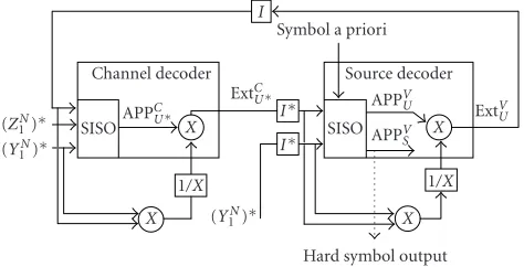
Figure 5: Joint source-channel decoding structure for a serial source-channel encoder (courtesy of [79]).
catenation of a source and a channel coder, as shown in Figure 4a.Figure 5shows the structure of the correspond-ing iterative decoder. InFigure 5, it is assumed that the chan-nel encoder is a systematic convolutional code with rate 1/2 that provides systematic bits, denoted byU1N, and redundant
bitsRN1. However, the principle applies similarly to channel
codes of different rates. Based on the schematic represen-tations given in Figure 4a, it has to be noted thatU1N
de-notes an interleaved sequence. After transmission through a noisy channel, the decoder receives the corresponding ob-servations, denoted byY1N andZ1N, respectively. InFigure 5,
the channel and source decoders are composed of soft-input soft-output (SISO) decoding components.3The SISO
com-ponents for the source decoder can be either a trellis decoder (e.g., using BCJR or SOVA algorithms) or a sequential de-coder, as described in Section 3.5. The two decoding com-ponents are separated by an interleaverIand a deinterleaver
I∗.4
3Note that additional bits can be used for terminating the trellis, but
this is not absolutely necessary. For instance, the results reported inFigure 9
are obtained considering uniform probabilities for initializing the different states of the RSC encoder in the BCJR backward recursion.
A first estimation (BCJR or SOVA) is run on the chan-nel decoder HMM with measuresY1N∗on the interleaved
se-quence of useful bits and the sese-quence of measures Z1N on
the redundant bits as inputs. It involves the computation of a sequence of APPs for the interleaved sequenceU1N∗ denoted
by APPCU∗. Then, the extrinsic information ExtCU∗
n relative to
each bitUn∗of the interleaved sequenceU1N∗ of useful bits is
computed from its posterior distribution obtained as a result of the channel decoding. The extrinsic information can be regarded as the modification induced by a new measurement (here all the measuresY1∗· · ·Y∗
N except for thelocaloneYn∗) on the APPs on the interleaved useful bitsUn∗conditioned by thelocalmeasurementYn∗. It can also be regarded as the in-cremental information on a current decoder state through the estimation of all the other decoder states. This extrinsic information is computed as
ExtCUn∗
Y∗=y∗|Y∗ n =yn∗
= P
U∗
n |Y∗=y∗
PU∗
n |Yn∗=y∗nExtVUn∗
Y∗=y∗|Y∗ n =y∗n,
(15)
where ExtVU∗ represents the interleaved sequence of the ex-trinsic information produced by the VLC decoder. Note that, when running the first channel SISO decoder (i.e., at itera-tion 0), this term simplifies as
ExtCUn∗
Y∗=y∗|Y∗
n =y∗n=P
U∗
n |Y∗=y∗
PU∗
n |Yn∗=y∗n
. (16)
If the estimation is run in a logarithmic domain, the extrinsic information is computed by subtracting the logarithm of the probability laws. Theextrinsicinformation on a useful bit is a direct subproduct of a BCJR algorithm or of a SOVA. In the case of sequential decoding, a conversion of the APP on the entire sequence of symbols (or equivalently states of the de-coder) into the APP of each useful bit, as expressed in (13), is needed. Notice that the motivation for feeding only extrin-sic information from one stage to the next is to maintain as much statistical independence between the bits as possible from one iteration to the next. As long as iterative decoding proceeds, and assuming sufficient interleaving, the reliabil-ity on states (or on transition bits) improves until it gets to a constant value. If the assumption of statistical independence is true, the iterative estimation on parts of the model each time approaches the MAP solution on the global model of dependencies as the number of iterations approaches infin-ity.
Thus, the channel decoder produces a sequence of extrin-sic information (ExtCU∗ = ExtCU∗
1 · · ·Ext C U∗
N) which is
dein-terleaved before being fed into the VLC decoder. A similar computation has to be carried out in the source decoder con-sidering the deinterleaved versions Y1N and ExtCU of the se-quences of measurements and extrinsic information. It, in turn, involves a computation of a sequence of APPs (APPVU) and yields another sequence of extrinsic information on the
B/S I∗ /
S/B / I
SISO channel decoder
Mean-square estimation SISO source
decoder ZN
1
ExtsK1 ExtV1N
APP∗V1N
Ext∗V1N ExtV1N
APPV1N YN
1 ZN1 YN
1
ZN
1
ˆ CK
1
Dem
ultiple
xer
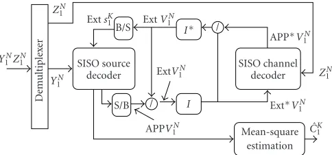
Figure6: Parallel iterative joint source-channel decoding structure.
useful bits:
ExtVUnY=y|Yn=yn
= P
Un|Y=y
PUn|Yn=ynExtCUn
Y=y|Yn=yn. (17)
The sequence ExtVU of extrinsic information is interleaved and then fed into the channel decoder. After a few iterations involving the two SISO decoders, the source decoder outputs the symbol estimates.
This principle has been very largely applied to joint source-channel coding and decoding of fixed-length [32] and variable-length (Huffman, RVLC, arithmetic, quasiarith-metic) codes. The convergence behavior of iterative source-channel decoding with fixed-length source codes and a serial structure is studied in [33] using extrinsic information trans-fer (EXIT) charts [34]. The gain brought by the iterations is obviously very much dependent on the amount of corre-lation present on both sides of the interleaver. The variants of the algorithms proposed for joint source-channel decod-ing of VLC-encoded sources relate to various forms of trellis representations for the source coder, as seen inSection 3, as well as to the different underlying assumptions with respect to the knowledge of the length of the sequences of symbols or of bits [12,13,14,17,20,21,35,52].
5.3. Parallel-concatenated joint source-channel decoding
A parallel-concatenated source-channel coding and decod-ing structure with VLC-encoded sources is described in [38]. In comparison with a parallel channel turbo coder, the ex-plicit redundancy from one channel coder is replaced by redundancy left in the source compressed stream U1N (see Figure 4b) after VLC encoding. The indexes of the quantized symbols are converted into a sequence of bitsV1M which is fed into a channel coder (possibly followed by a punctur-ing matrix to adjust the channel code rate). The channel coder produces the sequence of parity bitsRN1. The decoder
Extrinsic information on the binary representation of the quantized indexes, Ext(V1M), is then computed by
remov-ing (via a subtraction or a division dependremov-ing on whether the estimation is run in a logarithmic domain or not) the a priori information. The interleaved extrinsic information, Ext∗(V1M), is fed as a priori information to the soft-input soft-output channel decoder. Extrinsic information result-ing from the estimation run on the channel decoder model, after deinterleaving, is converted into a priori information on quantized symbols, which is fed in a second iteration to the soft-input soft-output source decoder. The authors in [38] show that, after the 20th iteration and for almost the same code rate (around 0.3), the parallel structure brings a gain that may be up to 3 dB in terms of SNR of the recon-structed source signal with respect to the serial structure. However, this result, that is, the superiority of the parallel versus serial structure, analogous to the comparison made between parallel and serial turbo codes [80], is limited to the case of a given RVLC code and to a AWGN channel with low SNRs.
6. SOURCE-CONTROLLED CHANNEL DECODING
Another possible approach is to modify the channel decoder in order to take into account the source statistics and the model associated to the source and source coder. A key idea presented in [39] is to introduce a slight modification of a standard channel decoding technique in order to take ad-vantage of the source statistics. This idea has been explored at first in the case of FLC and validated using convolutional codes in a context of transmission of coded speech frames over the global system of mobile telecommunication (GSM). Source-controlled channel decoding have also been applied with block and convolutional turbo codes, considering FLC for hidden Markov sources [40] or images [41,81,82,83]. The authors in [81], by first optimizing the turbo code poly-nomials, and second by taking into account source a pri-ori information in the channel decoder, show performances closer to the optimal performance theoretically achievable (OPTA) in comparison with a tandem decoding system based on Berrou’s rate-1/3 (37, 21) turbo code, for the same overall rate. However, when using FLC source codes, the ex-cess rate in the bit sequence fed into the channel coder is high. The source has not been compressed, and the channel code rate is high. To draw any conclusion on the respective advantages of joint versus tandem source-channel decoding techniques, one must consider the chain in which the source has been compressed as well. The freed bandwidth may then allow to reduce the channel code rate, hence increasing the error correction capability of the channel code. In this sec-tion, we show how the approach of source-controlled chan-nel decoding can be extended to cover the case of JSCD with VLC.
6.1. Source-controlled convolutional decoding with VLCs
Source-controlled channel decoding of VLC-coded sources has been first introduced in [42]. The transmission chain
considered is depicted in Figure 1: the source compressed stream produced by a VLC coder is protected by a convolu-tional code. The convoluconvolu-tional decoder proceeds by running a Viterbi algorithm which estimates the ML sequence. If we denote byX0N the sequence of states of the convolutional
en-coder, the ML estimation searches for the sequenceX0N such that P(Y1N|XN
0) is maximum. The ML estimate would be
equivalent to the MAP estimate if the source was equiproba-bly distributed, that is, if the quantityP(Xn|Xn−1) is constant.
However, here, the inputU of the channel coder is not in general a white sequence but a pointwise function of a Markov chain. The quantityP(Xn|Xn−1) is therefore not any
more constant, but has instead to be derived from the source statistics. One has in this case to use instead the generalized Viterbi algorithm [44] in order to get the optimal MAP se-quence, that is, the one minimizing the number of bit errors. For this, a one-to-one correspondence has to be maintained between each stage of the decoding path in the convolutional decoder and the vertex in the VLC tree [42] associated to the corresponding useful bitUnat the input of the channel coder. The probabilityP(Xn|Xn−1) is thus given by the transition
probability on the VLC codetree. For a first-order Markov source, to capture the intersymbol correlation, the probabil-ity P(Xn|Xn−1) becomes dependent on the last symbol that
has been coded, as explained inSection 3. The decoding al-gorithm thus proceeds with the search for the path that will maximize the metric
max χ P
XN
0|Y1N
⇐⇒max χ
N
n=1
lnPYn|Xn,Xn−1
+ ln N
n=1
PXn|Xn−1
, (18)
where χ denotes the set of all possible sequences of states for the channel decoding trellis [43,79]. Results reported in [42,84] show that though this method is suboptimal, it nev-ertheless leads to performances that are close to the ones pro-vided by the optimum MAP decoder [16], for which a prod-uct of the Markov source model, of the source coder, and channel coder model is computed.
6.2. Source-controlled turbo decoding with VLCs
Source-controlled turbo decoding can also be imple-mented for VLC compressed sources. In the transmis-sion system considered in [42, 84], the symbol stream
S1,S2,. . .,SK is encoded using a VLC followed by a system-atic turbo code which is a parallel concatenation of two convolutional codes. The transmitted stream, denoted by
U1,U2,. . .,UN,R1,R2,. . .,RN inFigure 1, now corresponds
to a sequence ofNtriplets, denoted by (Un,Rn,1,Rn,2), where
Undenotes the systematic bits andRn,1,Rn,2the parity bits
from the two constituent encoders. In contrast toSection 5,
UN
1 now designates a sequence of noninterleaved bits. In
![Figure 7: Parallel turbo decoding structure using a priori sourceinformation in the first decoder (courtesy of [79]).](https://thumb-us.123doks.com/thumbv2/123dok_us/1137556.1142683/14.600.51.292.73.197/figure-parallel-decoding-structure-priori-sourceinformation-decoder-courtesy.webp)
![Figure 10: Iterative source-channel decoding with online estimation (courtesy of [87]).](https://thumb-us.123doks.com/thumbv2/123dok_us/1137556.1142683/17.600.160.443.72.160/figure-iterative-source-channel-decoding-online-estimation-courtesy.webp)
