Volume 2006, Article ID 72879, Pages1–9 DOI 10.1155/ASP/2006/72879
Blind Adaptive Channel Equalization with
Performance Analysis
Shiann-Jeng Yu1and Fang-Biau Ueng2
1National Center for High Performance Computing, No. 21 Nan-Ke 3rd Road, Hsin-Shi, Tainan County 744, Taiwan 2Department of Electrical Engineering, National Chung-Hsing University, 250 Kuo-Kuang Road, Taichung 402, Taiwan
Received 4 March 2005; Revised 25 August 2005; Accepted 26 September 2005
Recommended for Publication by Christoph Mecklenbr¨auker
A new adaptive multiple-shift correlation (MSC)-based blind channel equalizer (BCE) for multiple FIR channels is proposed. The performance of the MSC-based BCE under channel order mismatches due to small head and tail channel coefficient is investigated. The performance degradation is a function of the optimal output SINR, the optimal output power, and the control vector. This paper also proposes a simple but effective iterative method to improve the performance. Simulation examples are demonstrated to show the effectiveness of the proposed method and the analyses.
Copyright © 2006 Hindawi Publishing Corporation. All rights reserved.
1. INTRODUCTION
Traditional adaptive equalizers are based on the periodic transmission of a known training data sequence in order to identify or equalize a distorted channel with intersym-bol interference (ISI). However, the use of training data se-quence may be very costly in some applications. Blind chan-nel equalizers (BCE) without training data available receive much attention in recent years [1–15]. Early blind equaliza-tion techniques [1, 2] exploited the higher order statistics (HOS) of the output to identify the channels. Unfortunately, the HOS-based BCE requires a large number of data samples and huge computation load which limit their applications in fast changing environments.
To circumvent the shortcomings of the HOS-based ap-proaches, second-order statistics (SOS) was considered in BCE. The SOS-based BCE was developed based on cyclo-stationary characteristics of the signal. The first SOS-based BCE was derived by Tong et al. [3]. They demonstrated that
the SOS is sufficient for blind adaptive equalization by
us-ing fractionally samplus-ing or usus-ing an array of sensors. Since that, extensive researches were explored in the literature. The well-known approaches are the least-squares, the
sub-space, and the maximum likelihood [3,8,9]. These blind
equalizers were termed the two-step methods which esti-mate multiple channel parameters first and then equalize the channels based on the estimated channel parameters. How-ever, the two-step methods are not optimal because they do not take the channel estimation error into account in the
second-step optimization procedure. Recently, direct equal-ization estimators become more attractive [10–13]. The lin-ear prediction-based equalizer was developed by [13]. Work
[12] used the adaptive beamforming technique to develop
a constrained optimization method. Multiple-shift correla-tion (MSC) of the signals can be used in a partially adaptive channel equalizer to achieve fast convergence speed and low computation load. These direct equalizers can be adaptive, leading to much simpler realization for practical implemen-tation.
The SOS-based equalizers have the advantages of fast convergence speed and lower computational complexity compared with the HOS-based approaches. Unfortunately,
most of the SOS-based equalizers suffer from the
perfor-mance degradation caused by the model mismatch. The mis-match may be from inadequate channel order estimation due to limited observation data or the small channel coefficients. Practical multipath channels often have small head and tail terms, selection of appropriate channel order may not be an easy task. As shown in [15] that the blind channel equaliza-tion/identification methods should model only the “signifi-cant part” of the channel composed of the “large” channel
coefficient terms. The “small” head and/or tail terms should
be neglected to avoid overmodeling the system and causing degradation of the equalization performance. Work [16] pre-sented a new channel order criterion for blind equalization
and [15] investigated the robustness of the LS and SS
In this paper, we study the steady-state performance of the MSC-based equalizer. We explore the relationship between the output signal-to-interference plus noise ratio (SINR) and the small head and tail terms of the FIR chan-nels. By applying an orthogonalization approximation to the analyses, the output SINR in terms of the small channel coef-ficients is derived. A degradation factor defined by the output SINR of the MSC-based equalizer over the optimal value is used to examine the performance degradation of the equal-izer. We find that the degradation factor is not only a
func-tion of the small channel coefficients, but also a function
of the optimal output SINR, the optimal output power, and the control vector. To reduce the degradation caused by the small channel coefficients, this paper proposes a simple itera-tive method. The analysis of the iteraitera-tive method is also per-formed. From the analysis results, we identify that the itera-tive method indeed improves the equalization performance.
2. SIGNAL MODEL
Let us consider an array withpantennas. If the received sig-nal is sampled at the symbol rate, the digitized data of the array can be written by [14],
y(n)= q
i=1
his(n−i+ 1) +z(n), (1)
wherey(n) = [y1(n)y2(n)· · ·yp(n)]T,{s(n)}is the input
signal symbol sequence, andz(n)=[z1(n)z2(n)· · ·zp(n)]T
is the additive white Gaussian noise vector. “T” represents the transpose.s(n) is an independent identically distributed (iid) zero-mean sequence with E{s(i)s∗(j)} = δ(i − j) and is independent ofzi(n). The channel parameters{hi = [h1(i)h2(i)· · ·hp(i)]T, i = 1, 2,. . .,q}contain all the
im-pulse response of thepFIR channels. The channel order of
this multiple FIR channel model of (1) isq−1. Define the data vectorYM(n)=[yT(n)yT(n−1)· · ·yT(n−M+ 1)]T, YM(n) can be expressed as
YM(n)=Bf(h)SM(n) +ZM(n), (2)
where
Bf(h)= ⎡ ⎢ ⎢ ⎢ ⎣
h1 h2 · · · hq · · · 0 ..
. . .. ... ... ... ...
0 · · · h1 h2 · · · hq ⎤ ⎥ ⎥ ⎥ ⎦
(pM)x(q+M−1)
= bf1,bf2,. . .,bf(q+M−1)
(3)
is a block Toeplitz matrix and is full rank. ZM(n) =
[zT(n)zT(n − 1)· · ·zT(n − M + 1)]T, S
M(n) =
[s(n)s(n − 1)· · ·s(n − q − M + 2)]T represents the signal sources corresponding to the columnsbf i(h).
The purpose of the equalizer is to provide an estimate of the signals(n−d+ 1) with a possible delay ofd−1 samples.
From beamforming point of view [16],s(n−d+ 1) can be
seen as the desired signal and the other signalss(n−i) with
i=d−1 can be virtually seen as the interferers. Tsatsanis
and Xu [12] noted the analogies of (2) to the beamforming
problem statement [16] and developed the COM for direct
blind equalizers. They found from (3) that ifM≥d−1≥q, bf d = [0 · · · 0 hTq hqT−1 · · · hT1 0 · · · 0]T
contain-ing the information of all channel parameters can be used in designing the blind equalizer. The COM algorithm can be derived through an optimization problem with multiple con-straints. Consider the optimization problem
min
WCOMW
H
COMRYMWCOM subject toCHdWCOM=h. (4)
The weight vector of the COM (constrained optimization method) algorithm is given by [12],
WCOM=R−YM1CdΦ−1θ, (5)
where Φ = CH
dR−YM1Cd, RYM = E{YM(n)YHM(n)}, θ is the
eigenvector ofΦcorresponding to the minimum eigenvalue,
and
Cd=
⎡ ⎢ ⎣
0p(d−q)×p(d−q)
Ipq×pq 0p(M−d)×p(M−d)
⎤ ⎥ ⎦
(pM)x(pq)
. (6)
From (5), the COM constructs pMadaptive weights to
estimate a total of pqchannel parameters for resolving one
of theM+q−1 signals ofSM(n). Unfortunately,pMis often
much greater thanM+q−1. For example, letp=10,q=3,
andM = 9, the number of adaptive weights for the COM
is as high as 90, but the number of all the signal sources of
SM(n) is only 11. Because the convergence speed and
com-putation load of an adaptive algorithm strongly depend on
the dimension of the adaptive weights [17], the COM using
such big number of adaptive weights to resolve a signal of SM(n) is not efficient. Another approach called the mutually referenced equalizers (MRE) [18] is based on the following observation. Without consideration of the noise, the equal-izers have
VH
kYM(n)=VHi YM(n+i−k)
fori,k=0, 1,. . .,q+M−1, k > i, (7)
where theVkare also defined ask-delay equalizers. There ex-ist equalizers to achieve perfect symbol recovery. However, in the presence of noise perfect symbol recovery is impossible by using the criterion of (7). Work [18] successfully devel-oped asymptotic algorithms for all equalization delays.
3. THE PROPOSED PARTIALLY ADAPTIVE CHANNEL EQUALIZER (PACE)
Consider a shift correlation matrix defined byRy(n,n−k)=
E{y(n)yH(n−k)}and is given by
Ry(n,n−k)=
q
i=1
q
j=1
Es(n−i+ 1)s∗(n−j−k+ 1)
×hihHj + E
Consider the algorithm for direct blind adaptive equaliza-tion using partially adaptive weights. Let Y(n) be a vector
containing the first N entries of YM(n) and be expressed
byY(n) = [yT(n)yT(n−1)· · ·yT(n−m+ 2)y
1(n−m+
1)y2(n−m+ 1)· · ·yl(n−m+ 1)]T, wherem= N/ pand
l=N−(m−1)p.·denotes the nearest larger integer. By (2) and (3),Y(n) can be written by
Y(n)=B(h)S(n) +Z(n), (9)
where theN×(q+m−1) matrixB(h) is written by
B(h)= ⎡ ⎢ ⎢ ⎢ ⎢ ⎢ ⎢ ⎢ ⎣
h1 h2 · · · hq · · · 0 0 ..
. . .. ... ... ... ... ...
..
. · · · h1 h2 · · · hq 0 0 · · · 0 ¯h1 ¯h2 · · · ¯hq
⎤ ⎥ ⎥ ⎥ ⎥ ⎥ ⎥ ⎥ ⎦
= b1,b2,. . .,bQ
,
(10)
whereQ=q+m−1 andbiis theith column ofB(h). It is noted thatB(h) is a submatrix ofBf(h) and is therefore full rank [19]. In (10), the vector¯hiconsists of the firstlentries ofhi,S(n)=[s(n)s(n−1)· · ·s(n−Q+ 1)]T, andZ(n)= [zT(n)· · ·zT(n−m+ 2)z
1(n−m+ 1)z2(n−m+ 1)· · ·zl(n−
m+1)]Tis aN×1 noise vector. The adaptive array theory [16]
states that aN-element array hasN−1 degrees of freedom
to resolve at mostN−1 signal sources including the desired signal and interference. Therefore, we have to select
N > Q (11)
to resolve one of the signal sources ofS(n). If the direction vectorbdis known, the optimal weight vector corresponding to the desired signals(n−d+ 1) is given by [16],
wd=μR−Y1bd, (12)
where RY(n) = E{Y(n)YH(n)} = B(h)BH(h) +σ2I andμ is a scalar. In this paper,μis used to normalize the weight vector. Since the direction vectorbd is probably containing a fraction of all the channel parameters, the equalizer using (12) is called the partially adaptive equalizer. Next, we use the MSC ofY(n) to find the weight vectorwd directly. Consider that
RY(n,n−k)=B(h)E
S(n)SH(n−k)BH(h)
+ EZ(n)ZH(n−k).
(13)
Thus, ifk=Q−1 andk≥m, (13) can be reduced to
RY(n,n−Q+ 1)=bQbH1. (14)
A simple method for extractingbQ from (14) is selecting a nonzero vectoru, which satisfiesbH1u=0. The direction
vec-torbQcan be found by
RY(n,n−Q+ 1)u=bQ
bH1u∝bQ. (15)
Similarly, consider another nonzero vectorvwithbHQv =0, then
RHY(n,n−Q+ 1)v=b1
bHQv
∝b1. (16)
By (12), (15), and (16), the weight vectors ofw1andwQcan be given by
wQ=μR−Y1(n)RY(n,n−Q+ 1)u∝R−Y1(n)bQ, w1=μR−Y1(n)RHY(n,n−Q+ 1)v∝R−Y1(n)b1.
(17)
The outputs corresponding to the zero-delay and (Q−
1)-delay signals are given bys(n)=wH1(n)Y(n) ands(n−Q+
1)=wHQ(n)Y(n), respectively. Using the same approach, the weight vectors ofwdford=2, 3,. . .,Q/2can be derived as follows:
wd=μRY−1(n)RY(n,n−Q+d)wQ, wQ+1−d=μRY−1(n)RHY(n,n−Q+d)w1,
(18)
wherewQ=μR−Y1(n)RY(n,n−Q+1)uandw1=μRY−1(n)RHY(n,
n−Q+ 1)v. It is noted that the above algorithm needs two initial vectorsuandvin (17) for calculatingw1andwQ,
re-spectively. In theory, any nonzero vectors havingbH
Qu = 0
andbH
1v = 0 can be chosen as the candidates. We can
se-lectu = wQ andv = w1 for consistency of the algorithm.
In the next section, we study the equalization performance in the presence of channels with small head and tail channel coefficients. We find that for the batch processing, selecting
u =wQ andv =w1has the benefit of improving the
per-formance. On the consideration of adaptive implementation of the proposed PACE algorithm, we first insert the time in-dex for the weight vectors for clarification. A straightforward thinking is to express (18) as follows:
wd(n)=μR−Y1(n)RY(n,n−Q+d)wQ(n), wQ+1−d(n)=μR−Y1(n)RHY(n,n−Q+d)w1(n).
(19)
Here, the algorithm cannot be implemented due to unavail-ability ofwQ(n) at this moment. For the recursive implemen-tation of the PACE, we slightly modify the above equations as
wd(n)=μR−Y1(n)RY(n,n−Q+d)wQ(n−1), wQ+1−d(n)=μR−Y1(n)RHY(n,n−Q+d)w1(n−1).
(20)
Let the correlation matrix be updated by
RY(n,n−k)=(1−α)RY(n−1,n−1−k)
whereαis a weighting factor with 0≤α≤1. The RLS-based PACE algorithm is summarized as follows:
R−1
Y (n)=
1 (1−α)R
−1
Y (n−1)
− α
(1−α)
R−Y1(n−1)Y(n)YH(n)R−Y1(n−1) (1−α)+αYH(n)R−1
Y (n−1)Y(n)
,
RY(n,n−Q+d)=(1−α)RY(n−1,n−1−Q+d)
+αY(n)YH(n−Q+d),
Pd(n)=RY(n,n−Q+d)wQ(n−1),
PQ+1−d(n)=RHY(n,n−Q+d)w1(n−1),
wd(n)=Wd(n)/Wd(n)
withWd(n)=RY−1(n)Pd(n), wQ+1−d(n)=WQ+1−d(n)/WQ+1−d(n)
withWQ+1−d(n)=RY−1(n)PQ+1−d(n),
(22)
withR−1
Y (0)=τIandwQ(0)=uandw1(0)=v. Here,τis a
very large scalar. The computational complexity isO(N2).
3.1. A new order detection criterion
Now consider that
k=trace
RYH(n,n−k)RY−1RY(n,n−k)
, (23)
we have
k= ⎧ ⎨ ⎩
hq2
hH
1R−Y1h1
, ifk=q−1,
0, ifk≥q, (24)
wherehidenotes the 2-norm ofhi. Sincehiis not zero,
kmay be an indicator for determining the order of the FIR
channels by checking its value nonzero. However, at practical situation of finite number of samples, we have
k=traceRHY(n,n−k)R−Y1RY(n,n−k)
=
p
i=1
gk(i), (25)
wheregk(i)=PHi R−Y1PiwithPitheith column ofRY(n,n−
k). In practice,k will never be zero for anyk. Therefore detecting the channel order by nonzero check criteria should be modified for the finite-sample examples.
Here, we observe that the values ofkfork≥qshould
not have very significant difference at sufficient large number
of samples. We suppose thatk fork ≥ qare in the same
hypothesis termedH0. On the other hand,q−1should be in
another hypothesis termedH1. Now consider the following
parameter:
Υk=
k
1/(K−k) Ki=k+12i
, (26)
Table1: Channel impulse response of 4-element array.
Antenna h0∗103 h1∗103 h2 h3
#1 4.091ej(−0.019) 9.06ej(−0.41) 0 1.31ej(0.23)
#2 2.47ej(0.58) 18.4ej(−1.25) 1.31ej(−0.23) 1.16ej(1.48)
#3 2.74ej(−0.91) 6.9ej(0.92) 0 0.62ej(−1.11)
#4 1.39ej(−0.03) 18.4ej(−1.46) 0.52ej(−1.13) 0.21ej(−1.43)
Antenna h4 h5 h6∗103 h7∗103
#1 2.87ej(0.98) 0.32ej(0.96) 5.77ej(−1.16) 2.56ej(0.31)
#2 2.09ej(1.01) 0.75ej(0.68) 3.95ej(0.019) 1.35ej(1.28)
#3 1.21ej(−1.08) 0.15ej(−0.98) 13.08ej(−0.98) 1.54ej(−0.74)
#4 0.95ej(−1.07) 0.31ej(−0.95) 15.06ej(0.88) 0.37ej(−1.28)
whereKis chosen as a sufficient large integer so thatK > q. Sincek, forK ≥k≥q, do not have significant difference,
the denominator and the nominator of (26) should be
ap-proximately equal. It follows thatΥkshould be around 1 for
K ≥ k ≥ q. On the contrary, sinceq−1 should be
signif-icantly greater thank forK ≥ k ≥ q,Υq−1 should be a
significant large value comparing toΥkfork≥q. Therefore, we propose a detection criterion by
Υk ⎧ ⎨ ⎩
≥η, forkinH1,
< η, forkinH0,
(27)
whereη is a detection threshold. The channel orderqcan
be determined byq =k+ 1 ifΥk ≥η. As a fact, largeK is preferred, but largeKleads to more computations for finding allΥkfor order detection.
It is known thatRY(n,n−k) is the maximum likelihood estimate ofRY(n,n−k) [17]. From the first and second as-sumptions of this paper, we know that{s(n)}is a zero-mean iid random sequence and{vi(n)}is the additive zero-mean white Gaussian noise. Using the central limit theorem [20], eachgk(i) can be asymptotically modeled as an independent
χ2random variable for sufficient largeL[21].
kis the sum ofgk(i) and should have theχ2distribution. According to the
probability theory [20],Υ2
khas theF(1,K−k) distribution or±Υkhas thet-distribution with degrees of freedomK−k. Sincek, forK ≥k≥q, are of the hypothesisH0, we have
−η < ±Υk < ηor equivalentlyΥk < ηat a specified
confi-dence level. The range (−η,η) is called the confidence inter-val at a specified confidence level. In general, 90% or 95%
confidence levels are commonly used. Table 3 presents the
threshold with 90% and 95% confidence levels, whereηis
a function ofK−kand can be written byη=η(K−k). Since
q−1is not of the hypothesisH0,Υq−1should violate the rule
ofΥq−1 < η. At that time, the orderq can be detected. We
summarize the proposed order detection procedure as fol-lows.
Step 1. Select the threshold valueηbased on a specified con-fidence level and select a sufficient large integerK.
Step 2. Computekby (25) fork=K,K−1,. . ., 1.
Table2: Channel impulse response of 6-element array.
Antenna h1 h2 h3 h4
#1 0.02ej(−0.07) 0.13ej(0.45) 1.29ej(−0.98) 0.85ej(−0.019)
#2 2.08ej(−0.97) 1.21ej(0.78) 1.31ej(−1.28) 0.85ej(1.11)
#3 0.06ej(−0.02) 0.45ej(−0.52) 0.43ej(−0.99) 0.28ej(−0.019)
#4 0.02ej(−0.19) 1.091ej(−0.33) 0.29ej(−1.019) 0.19ej(0.89)
#5 0.15ej(0.79) 0.25ej(−0.79) 0.24ej(−0.78) 0.18ej(−0.19)
#6 0.008ej(−0.02) 0.05ej(−0.55) 0.09ej(−1.019) 0.09ej(−0.29)
Step 4. IfΥk< η,k=k−1 and go back toStep 3.
Step 5. IfΥk≥η,q=k+ 1 and stop the procedure.
In general, at least a signal source ofS(n) will be resolved in equalization. The minimum criterion for the PACE to equalize the channels and resolve at least two signal sources isq+m−2 ≥ m, that is,q ≥ 2. It shows that if at least a multipath signal is present in the environment, the PACE al-gorithm using (17) can resolve the zero-delay and (q−m +2)-delay signals ofS(n).
More generally, the PACE algorithm can resolve any sig-nal source ofS(n) if the time-shift indexksatisfiesk ≥ m. From descriptions of the previous subsection, the minimal
multiple-shift index k required for resolving all the signal
sources isk=q+m−1− (q+m−1)/2. As a result, the constraint for resolving all the signal sources ofS(n) is given by
q+m−1−
q
+m−1
2
≥m, (28)
wherem= N/ p. Both (11) and (28) provide designers con-straints of the dimension of the partially adaptive weightsN
to achieve channel equalization.
4. STEADY-STATE PERFORMANCE ANALYSIS
For the batch processing, the initial vectors uandvwhich
satisfy with the constraints shown in the above section can achieve the same performance. However, in the presence of channel with small head and tail channel coefficients [22], the performance is different. In this section, we study the ef-fect of the initial vectorsuandvin the steady-state with small channel coefficients. A method for selecting the initial vec-tors is proposed and its performance is also studied. Let us consider a performance index called the output SINR which is defined as follows:
ξd=
wHdbdbHdwd wHdRY −bdbHd
wd
(29)
for estimating the (d−1)-delay signal source ofY(n), that is,s(n−d+ 1), by usingwd, wherewHdbdbHdwdis called the output signal power corresponding tos(n−d+ 1).
4.1. Analysis
It has been assumed that the direction vectors ofb1,b2,. . .,
bm1andbQ,bQ−1,. . .,bQ−m2+1are small comparing with the
direction vectors ofbm1+1,bm1+2,. . .,bQ−m2. The weight
vec-tors are
wm1+1=R −1
Y (n)RHY
Q−m1−m2−1
u, (30)
where
RY
Q−m1−m2−1
=
m1+m2+1
i=1
bQ−m1−m2−1+ibHi . (31)
Substituting (31) into (30) yields
wm1+1=
m1+m2+1
i=1
R−1
Y (n)bibHQ−m1−m2−1+iu. (32)
Using (32), we have
bH
m1+1wm1+1=
m1+m2+1
i=1
bH
m1+1R
−1
Y (n)bibQH−m1−m2−1+iu
≈po(m1+1)b
H
Q−m2u,
(33)
wherepo(m1+1) =b
H
m1+1R
−1
Y (n)bm1+1and|b
H
m1+1R
−1
Y (n)bi|
bHm1+1R −1
Y (n)bm1+1. Therefore, its term can be neglected with
comparison to the term withbHm1+1R −1
Y (n)bm1+1. The output
power of usingwm1+1is given by
wH
m1+1RY(n)wm1+1
=
m1+m2+1
i=1,j=1
uHb
Q−m1−m2−1+ibHi R−Y1(n)bjbHQ−m1−m2−1+ju
≈
m1+m2+1
i=1
poiuHbQ−m1−m2−1+i2.
(34)
The output SINR ofwm1+1is given by
ξm1+1=
wmH1+1bm1+1b
H
m1+1wm1+1
wmH1+1
RY(n)−bm1+1b
H
m1+1
wm1+1
. (35)
After some calculations, we have ξm1+1 ≈ ξo(m1+1)Ψm1+1,
whereξo(m1+1)is the optimal SINR and
Ψ−1
m1+1=1 +
ξo(m1+1)
po(m1+1)
×
⎛ ⎜ ⎝
m1+m2+1
i=1,i=m1+1poiu
Hb
Q−m1−m2−1+i
2
po(m1+1)bHbQ−m2
2
⎞ ⎟ ⎠
(36)
being in terms of the effect of the performance due to small heads and small tails of the channel parameters.
4.2. Selecting initial vectors
Table3: The detection threshold of thet-distribution with 90% and 95% confidence interval.
K−k 1 2 3 4 5 6 7 8 9 ∞
90% 6.314 2.920 2.353 2.132 2.015 1.943 1.985 1.860 1.833 1.645 95% 12.706 3.182 2.776 2.571 2.447 2.365 2.306 2.262 2.228 1.960
of the adaptive spatial filtering. Letwm1+1(l) andwQ−m2(l)
represent the weight vectors afterliterations. The iterative method is described as follows:
wm1+1(l)=R −1
Y (n)RHY
Q−m1−m2−1
u(l),
wQ−m2(l)=R−
1
Y (n)RY
Q−m1−m2−1
v(l). (37)
Letu(l)=wQ−m2(l−1) andv(l)=wm1+1(l−1). We have
wm1+1(1)=R −1
Y (n)RHY
Q−m1−m2−1
u(1), (38)
wm1+1(2)=Φv(1), (39)
where
Φ=R−1
Y (n)RHY
Q−m1−m2−1
R−1
Y (n)RY
Q−m1−m2−1
≈
m1+m2+1
i=1
po(Q−m1−m2−1+i)R−Y1(n)bibHi .
(40)
By (38), we can find that
wm1+1(2l+ 1)=Φ
lR−1
Y (n)RHY
Q−m1−m2−1
uwm1+1(2l) =Φlv(1).
(41)
And we can approximateΦlby
Φl≈
m1+m2+1
i=1
plo(Q−m1−m2−1+i)poil−1R−Y1(n)bibHi . (42)
The output SINR after (2l+ 1) iterations can be found by
ξm1+1(2l+ 1)≈ξo(m1+1)Ψm1+1(2l+ 1), (43)
where
Ψ−1
m1+1(2l+ 1)
=1 + $ξ
o(m1+1)
po(m1+1)
%
×
⎛ ⎜ ⎝
m1+m2+1
i=1,i=1 p2
l
o(Q−m1−m2−1+i)p2oil+1uHb(Q−m1−m2−1+i)2
p2l
o(Q−m2)p
2l+1
o(m1+1)u
Hb
Q−m2
2
⎞ ⎟ ⎠.
(44)
5. SIMULATION RESULTS
In this section, computer simulations are performed to eval-uate the proposed blind equalizer. The COM and MRE are also performed for comparison.
10−5
10−4
10−3
10−2
10−1
100
The
p
er
fo
rmanc
e
fact
o
r
5 10 15 20 25 30 35 40
Input SNR (dB) With 20 iterations
Without iteration
Figure1: The performance factor versus the input SNR with the theoretical results (solid curve) and the experimental results (∗).
−20
−15
−10
−5 0 5
The
p
er
fo
rmanc
e
fact
o
r
(dB)
2 4 6 8 10 12 14 16 18 20
Iterations (#)
Figure2: The performance factor versus iterations for the batched PACE with the theoretical results (solid curve) and the experimental results (∗).
5.1. Batch processing
To show the effectiveness of our proposed iterative method, we employ a 4-element array with channel parameters shown in Table 1. It is noted that the channel has 2 small leading
and tail channel responses. That is, m1 = m2 = 2. The
−25
−20
−15
−10
−5 0 5 10 15 20
Output
SINR
(dB)
0 100 200 300 400 500 600 700 800 900 1000 Number of samples
With 20 iterations
Without iteration Batched PACE with delay=0
Figure3: The output SINR versus the number of samples for the batched PACE.
as 4 for the proposed algorithm. Thus, we have Q = 11.
Figure 1shows the performance degradation at different
in-put SNR. It is shown that the iterative method using (37)
significantly improves the performance. The PACE without iteration is quite sensitive to the small leading and tail terms. The performance analysis approaches to the experimental
result.Figure 2shows the performance at different number
of iterations. The input SNR is 20 dB. We find from these figures that the PACE with iterations can significantly in-crease the output SINR. However, using iterations more than 15, the improvement is quite limited. Next, let us exam the performance for finite number of samples. The iid BPSK signal with values{+1,−1}is passed through the channels and received by the array. The correlation matrix is calcu-lated by
RY(n,n−k)= 1
K
K−1
i=0
Y(n−i)YH(n−k−i) (45)
withKdata samples.Figure 3shows the results of the PACE
with and without iterations. The input SNR is 20 dB. The results are obtained by averaging 100 independent runs. We find that the PACE without iteration does not have good per-formance. The iterative approach can significantly improve the performance. For the channel order detection problems,
we chooseK = 8. The detection thresholds with 90% and
95% confidence levels shown in Table 3 are used for
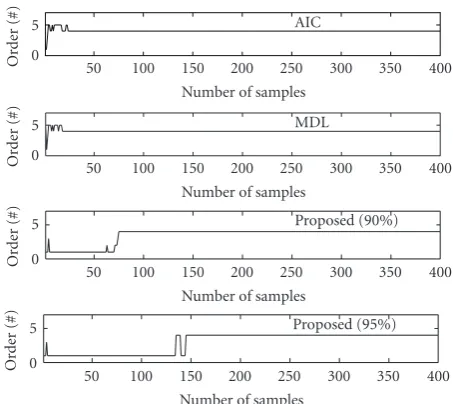
sim-ulations.Figure 4presents the results of the channel order detection of the proposed method with 90% and 95% con-fidence levels and the AIC and MDL. The input
signal-to-noise ratio (SNR) is 20 dB.Figure 4shows that the AIC and
MDL require about 30 samples to detect correct channel or-der. But the proposed method using both 90% and 95% con-fidence levels requires about 70 and 150 samples, respectively,
to achieve the same performance.Figure 5shows the
detec-tion probability versus the number of samples. The results
0 5
Or
der
(#)
50 100 150 200 250 300 350 400 Number of samples
AIC
0 5
Or
der
(#)
50 100 150 200 250 300 350 400 Number of samples
MDL
0 5
Or
der
(#)
50 100 150 200 250 300 350 400 Number of samples
Proposed (90%)
0 5
Or
der
(#)
50 100 150 200 250 300 350 400 Number of samples
Proposed (95%)
Figure 4: Detection of the channel order using the proposed method and the AIC and MDL.
are calculated from 100 independent runs. The input SNR is 20 dB. We find that the MDL is the most efficient method and can detect correct channel order using small number of sam-ples to achieve very high detection probability (over 90% de-tection probability). The AIC often overestimates the chan-nel order and its detection probability cannot reach a very high probability. The proposed method using 90% and 95% confidence levels works better than the AIC and can achieve very high detection probability if the number of samples is
sufficient large. This example shows that using 95%
confi-dence level is too conservative to detect channel order with high detection probability at limited number of samples. On the contrary, the 90% confidence level is more moderate for this example.Figure 6presents the detection probability in
different input SNR values. The results are calculated from
100 independent runs. The number of samples used in this example is 200. We find that the MDL is very sensitive to vari-ations of the input SNR. It cannot reach high detection prob-ability at low input SNR. In contrast, the proposed method using 90% confidence level is robust to variations of the SNR
comparing to the AIC and MDL. At SNR=5 dB, it can
de-tect correct channel order with more than 70% probability. In this figure, the proposed method using 95% confidence level does not have satisfactory results at low SNR. From
Fig-ures5and6, we can conclude that the proposed order
de-tection method (e.g., using the 90% confidence level) is not sensitive to variations of the input SNR, but is sensitive to the number of samples. In general, the large number of samples is required for the proposed method to detect the channel order with high detection probability.
5.2. Adaptive processing
To investigate the PACE algorithm of using (20), we consider
an array with p = 6 antenna elements. A channel impulse
0 0.2 0.4 0.6 0.8 1
Det
ection
p
ro
babilit
y
50 100 150 200 250 300 350 400 Number of samples
MDL
AIC 90%
95%
Figure5: The detection probability versus the number of samples.
0 0.2 0.4 0.6 0.8 1
Det
ection
p
ro
babilit
y
5 10 15 20 25 30
Input SNR (dB) MDL
AIC 90%
95%
Figure6: The detection probability versus the input SNR.
for this case. The multiplicitymis chosen as 4 for PACE and MRE and as 6 for the COM. At the beginning of the iteration, the initial weight vectors ofw1(0) andw7(0) of the PACE are
set as nonzero random vectors for each independent run. The weighting factor is chosen asα=1/n.Figure 7presents the output SINR versus the number of samples. The results are obtained by averaging by 100 independent runs. The PACE algorithm has fast convergent speed and achieves very good performance. The PACE has performance better than that of
the MRE and COM. We note from (12) that the channel
pa-rameters can be estimated from the weight vector. The weight vectorwq∝R−Y1bq. Therefore,bq=ηRY(n)wq, whereηis a complex variable for gain and phase adjustment. Ifm=4, we havebq=[hT4 h3T hT2 hT1]T. All the channel parameters can
be estimated frombq.Figure 8shows the mean square error
(MSE) of the estimated channel parameters. The COM with
−20
−15
−10
−5 0 5 10 15 20
Output
SINR
(dB)
0 100 200 300 400 500 600 700 800 900 1000 Number of samples
Figure7: The output SINR versus the number of samples. Solid curve: the PACE, dash curve: the COM, dash-dot curve: the MRE.
10−3
10−2
10−1
100
101
MSE
0 100 200 300 400 500 600 700 800 900 1000 Number of samples
Figure8: The MSE versus the number of samples. Solid curve: the PACE, dash-curve: the COM.
delay 4 andM =6 is used for comparison.Figure 8shows
that the PACE outperforms the COM.
6. CONCLUSIONS
An effective order detection method and a PACE algorithm
for direct multichannel equalization have been presented. Both of the order detection method and the PACE algo-rithm use the MSC property of the data. The order detection
method is derived from the MSC matrix. At
-distribution-based hypothesis testing criteria is used for detecting the
channel order. The proposed method can effectively detect
detection method to have high detection probability. We have found from the analyses that the weight vector which yields higher output SINR is more sensitive to the small channel
coefficients. In order to reduce the performance degradation
caused by the small channel coefficients and the control vec-tor, we propose a simple iterative method. The performance improvement of the iterative method has also been analyzed.
REFERENCES
[1] G. B. Giannakis and J. M. Mendel, “Identification of non-minimum phase systems using higher order statistics,”IEEE Transactions on Acoustics, Speech, and Signal Processing, vol. 37, no. 3, pp. 360–377, 1989.
[2] B. Porat and B. Friedlander, “Blind equalization of digital communication channels using high-order moments,”IEEE Transactions on Signal Processing, vol. 39, no. 2, pp. 522–526, 1991.
[3] L. Tong, G. Xu, and T. Kailath, “Blind identification and equal-ization based on second-order statistics: a time domain ap-proach,” IEEE Transactions on Information Theory, vol. 40, no. 2, pp. 340–349, 1994.
[4] D. T. M. Slock, “Blind fractionally-spaced equalization, perfect-reconstruction filter banks and multichannel linear prediction,” inProceedings of IEEE International Conference on Acoustics, Speech, and Signal Processing (ICASSP ’94), vol. 4, pp. 585–588, Adelaide, SA, Australia, April 1994.
[5] M. Gurelli and C. L. Nikias, “EVAM: an eigenvector-based al-gorithm for multichannel blind deconvolution of input col-ored signals,”IEEE Transactions on Signal Processing, vol. 43, no. 1, pp. 134–149, 1995.
[6] E. Moulines, P. Duhamel, J.-F. Cardoso, and S. Mayrargue, “Subspace methods for the blind identification of multichan-nel FIR filters,”IEEE Transactions on Signal Processing, vol. 43, no. 2, pp. 516–525, 1995.
[7] H. Liu and G. Xu, “Closed-form blind symbol estimation in digital communications,”IEEE Transactions on Signal Process-ing, vol. 43, no. 11, pp. 2714–2723, 1995.
[8] G. Xu, H. Liu, L. Tong, and T. Kailath, “A least squares-approach to blind channel identification,”IEEE Transactions on Signal Processing, vol. 43, no. 12, pp. 2982–2993, 1995. [9] Y. Hua, “Fast maximum likelihood for blind identification of
multiple FIR channels,”IEEE Transactions on Signal Processing, vol. 44, no. 3, pp. 661–672, 1996.
[10] G. B. Giannakis and S. D. Halford, “Blind fractionally spaced equalization of noisy FIR channels: direct and adaptive solu-tions,”IEEE Transactions on Signal Processing, vol. 45, no. 9, pp. 2277–2292, 1997.
[11] G. B. Giannakis and C. Tepedelenlioglu, “Direct blind equaliz-ers of multiple FIR channels: a deterministic approach,”IEEE Transactions on Signal Processing, vol. 47, no. 1, pp. 62–74, 1999.
[12] M. K. Tsatsanis and Z. Xu, “Constrained optimization meth-ods for direct blind equalization,”IEEE Journal on Selected Ar-eas in Communications, vol. 17, no. 3, pp. 424–433, 1999. [13] J. Mannerkoski and D. P. Taylor, “Blind equalization using
least-squares lattice prediction,”IEEE Transactions on Signal Processing, vol. 47, no. 3, pp. 630–640, 1999.
[14] L. T. Tong and Q. Zhao, “Joint order detection and blind chan-nel estimation by least squares smoothing,”IEEE Transactions on Signal Processing, vol. 47, no. 9, pp. 2345–2355, 1999.
[15] Q. Zhao and L. T. Tong, “Adaptive blind channel estima-tion by least squares smoothing,”IEEE Transactions on Signal Processing, vol. 47, no. 11, pp. 3000–3012, 1999.
[16] R. T. Compton Jr.,Adaptive Antennas, Concepts, and Perfor-mance, Prentice-Hall, Englewood Cliffs, NJ, USA, 1988. [17] R. Monzingo and T. Miller,Introduction to Adaptive Arrays,
John Wiley & Sons, New York, NY, USA, 1980.
[18] D. Gesbert, P. Duhamel, and S. Mayrargue, “On-line blind multichannel equalization based on mutually referenced fil-ters,”IEEE Transactions on Signal Processing, vol. 45, no. 9, pp. 2307–2317, 1997.
[19] G. H. Golub and C. F. Van Loan,Matrix Computations, Johns Hopkins University Press, Baltimore, Md, USA, 1983. [20] P. G. Hoel, S. C. Port, and C. J. Stone,Introduction to
Probabil-ity Theory, Houghton Mifflin, Boston, Mass, USA, 1971. [21] A. B. Baggeroer, “Confidence intervals for regression (MEM)
spectral estimates,”IEEE Transactions on Information Theory, vol. 22, no. 5, pp. 534–545, 1976.
[22] A. P. Liavas, P. A. Regalia, and J.-P. Delmas, “Blind channel approximation: effective channel order determination,”IEEE Transactions on Signal Processing, vol. 47, no. 12, pp. 3336– 3344, 1999.
Shiann-Jeng Yureceived the Ph.D. degree from the National Taiwan University in electrical engineering in 1995. From Octo-ber 1995 to DecemOcto-ber 2001, he was with National Space Program Office (NSPO) of Taiwan as an Associate Researcher. From January 2001 to July 2002, he was with the National Science Council (NSC) as a Specialist Secretary of vice chairman office. Since August 2002, he has been with the
Na-tional Center for High Performance Computing (NCHC). He is now a NCHC Deputy Director at the south region office. His spe-cialties and interests are digital signal processing, wireless commu-nication and satellite commucommu-nication, and grid computing and ap-plications in e-learning.
Fang-Biau Uengreceived the Ph.D. degree in electronic engineering from the National Chiao Tung University, Hsinchu, Taiwan in 1995. From 1996 to 2001, he was with Na-tional Space Program Office (NSPO) of Tai-wan as an Associate Researcher. From 2001 to 2002, he was with Siemens Telecommu-nication Systems Limited (STSL), Taipei, Taiwan, where he was involved in the design of mobile communication systems. Since