A Comparative Study on Seismic Incoherent SSI Analysis Methodologies

COMPARATIVE STUDIES ON SEISMIC INCOHERENT

SSI ANALYSIS METHODOLOGIES

Dan M. Ghiocel1

1

Ghiocel Predictive Technologies, Inc., Rochester, New York, USA ([email protected])

ABSTRACT

The paper discusses the effects of the 3D seismic random wave propagation (incoherent motion) vs. the 1D seismic deterministic wave propagation (coherent motion) on SSI response. Both theoretical and practical aspects are presented. The presented incoherent SSI analyses were performed using deterministic and stochastic incoherent SSI approaches with and without complex response phase adjustment as implemented in the ACS SASSI code (Ghiocel, 2013). The incoherent SSI approaches with phase adjustment were validated by EPRI (Short, Hardy, Merz and Johnson, 2007) and accepted by US NRC (2008) for their application to the seismic SSI analysis of the new nuclear power plant structures in United States. The paper investigates the effects of complex response phasing on the incoherent in-structure response spectra (ISRS) for different nuclear island SSI models. It is shown that EPRI validated incoherent SSI approaches are always conservative, but sometimes they could be overly conservative for complex FEA SSI models. Finally, the effect of the foundation basemat flexibility that increases the incoherent ISRS and the bending moments in the baseslab is discussed.

MATHEMATICAL MODELING OF SEISMIC MOTION INCOHERENCY

It should be understood that the traditional coherent motion inputs for SSI analysis comes from the 1D vertically S and P wave propagation assumption that has been accepted in the nuclear engineering practice for the last few decades. Based on the vertically propagation assumption, the coherent motion at the ground surface is described by a “rigid body” motion for which all the point motions under the foundation footprint are in phase. In contrast to simplified representation of the seismic wave field by coherent motion, incoherent motions idealize the 3D seismic random wave fields, including inclined body waves and surface waves, based on existent dense array ground acceleration records. Incoherent motions are nothing else than realistic 3D wave motion simulations based on the stochastic models developed from the 3D wave dense array record databases. Thus, incoherent motions are much more realistic representations of seismic ground motion than coherent motions.

Seismic motion incoherency is produced by the local random spatial variation of ground motion in horizontal plane in the vicinity of building foundations. To capture the spatial variability of the ground motion in horizontal plane, a stochastic field model is required. Assuming that the spatial variation of the ground motion at different locations could be defined by a homogeneous Gaussian stochastic field, its spatial variability is completely defined by its coherency spectrum, or coherence function.

Incoherent Free-Field Motion

The coherent free-field motion at any interaction node dof k,U ( )g,c_k ω is computed by:

g,c g,c g

k k 0

where H ( )g,c ω is the (deterministic) complex coherent ground transfer function vector at interface nodes

and U ( )g₀ ω is the complex Fourier transform of the control motion. Similarly, the incoherent free-field

motion at any interaction node dof k,U ( )g,i_k ω is computed by:

g,i g,i g

k k 0

U ( )ω =H ( )U ( )% ω ω (2)

where H ( )%g,i ω is the (stochastic) incoherent ground transfer function vector at interaction node dofs and

g 0

U ( )ω is the complex Fourier transform of the control motion. The main difference between coherent

and incoherent free-field transfer function vectors is that the H ( )g,c ω is deterministic quantity while g,i

k

H ( )% ω is a stochastic quantity (the tilda represents a stochastic quantity) that includes deterministic effects due to the seismic plane-wave propagation, but also stochastic effects due to incoherent motion spatial variation in horizontal plane. Thus, the incoherent free-field transfer function at any interaction node can be defined by:

g,i k

H ( )% ω g,c

k k

S ( )H ( )

= ω ω (3)

where S ( )_k ω is a frequency-dependent quantity that includes the effects of the stochastic spatial variation of free-field motion at any interaction node dof k due to incoherency. In fact, in the numerical implementation based on the complex frequency approach, S ( )_k ω represents the complex Fourier transform of relative spatial random variation of the motion amplitude at the interaction node dof k due to incoherency. Since these relative spatial variations are random,S ( )_k ω is stochastic in nature. The

stochastic S ( )_k ω can be computed for each interaction node dof k using spectral factorization of coherency matrix computed for all SSI interaction nodes. For any interaction node dof k, the stochastic spatial motion variability transfer function H ( )%g,i_k ω in complex frequency domain is described by the product of the stochastic eigen-series expansion of the spatial incoherent field times the deterministic complex coherent ground motion transfer function:

g,i k H ( )% ω

M

g,c

j,k j j k

j 1

[

( ) ( )

( )]H ( )

=

=

_∑

Φ

ω λ ω η ω

ω

where λ ω_j( ) and

Φ

( )

ω

k. The factor η ω_θj( ) is the random phase component associated with the j-th eigenvector that is given by

j( ) exp(i )j

θ

η ω = θ in which the random phase angles are assumed to be uniformly distributed over the unit circle. The number of coherency matrix eigenvectors, or incoherency spatial modes, could be either all modes or a reduced number of modes M depending on the eigen-series convergence. If only a limited number of incoherency spatial modes are used, then, the incoherent SSI response could be less accurate, as shown hereafter.

Incoherent SSI Response Calculations

For a coherent motion input, assuming a number of interaction nodes equal to N, the complex Fourier SSI response at any structural dof i, U ( )s,c_i ω , is computed by the superposition of the effects produced by the application of the coherent motion input at each interaction node k:

N N

s,c s g,c s g,c g

i i,k k i,k k 0

k 1 k 1

U ( ) H ( )U ( ) H ( )H ( )U ( )

= =

where the H ( )s ω matrix is the structural complex transfer function matrix given unit inputs at interaction

node dofs. The component

H ( )

ω

unit amplitude motion at the k-th interaction node dof is applied. For incoherent motion input, the complex Fourier SSI response at any structural dof i, U ( )s,i_i ω , is computed similarly by the superposition of the effects produced by the application of the incoherent motion input at each interaction node dof k:

N N M

s,i s g,i s g,c g

i i,k k i,k j,k j j k 0

k 1 k 1 j 1

U ( )

H ( )U ( )

H ( )[

( ) ( )

( )] H

( )U ( )

= = =

ω =

_∑

ω

ω =

_∑

ω

_∑

Φ

ω λ ω η ω

ω

ω

Two types of incoherent seismic SSI analysis approaches are available, namely, stochastic and deterministic approaches. Different incoherent SSI approaches were investigated by EPRI (Short, Hardy, Merz and Johnson, 2007). Stochastic approach is based simulating random incoherent motion realizations (Simulation in EPRI studies). Using stochastic simulation algorithms, a set of random incoherent motion samples is generated at each foundation SSI interaction nodes. For each incoherent motion random sample an incoherent SSI analysis is performed. The final mean SSI response is obtained by statistical averaging of SSI response random samples. Deterministic approach approximates the mean incoherent SSI response using simple superposition rules of random incoherency mode effects, such as the algebraic sum (AS) (AS in EPRI studies) or the square-root of the sum of square (SRSS) (SRSS in EPRI studies).

It should be noted that the EPRI validated incoherent SSI approaches include a conservative assumption that the incoherent complex response phases are zero or very close to zero. This makes EPRI validated approaches conservative with respect to the incoherent ISRS computation. As shown in this paper, the zero phase assumption produces only a slightly conservative solution for simple stick SSI models, as the SSI models used in the EPRI studies (Short, Hardy, Merz and Johnson, 2007), but an overly conservative solution for complex FEA SSI models.

The ACS SASSI code (Ghiocel, 2013) used for the investigations presented in this paper incorporates incoherent SSI approaches with and without phase adjustment, i.e. with zero or non-zero complex response phases. Using ACS SASSI, the effect of complex response phasing was investigated as shown in this paper.

APPLICATION CASES AND INCOHERENT SSI RESPONSE MODELING STUDIES

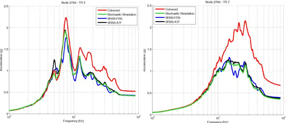
A typical comparison between coherent and incoherent ISRS computed for a Reactor Building (RB) complex computed using different incoherent SSI approaches is shown in Figure 1. The RB complex was idealized as multibranch stick model with a rigid foundation baseslab. The site was a rock site. The 2007 Abrahamson coherence function was used (Abrahamson, 2007).

Figure 1 Coherent vs. Incoherent ISRS Computed for Large-Size Footprint RB Complex Using EPRI Validated Approaches, Stochastic Simulation, SRSS ATF and SRSS ISRS

Effect of Using A Limited Number of Incoherency Spatial Modes

It should be noted that the use of all incoherency eigenmodes produces an “exact” recovery of the free-field coherency matrix at the foundation interaction nodes. Except SRSS, the other EPRI incoherent SSI approaches such as AS and Simulation include all incoherency eigenmodes. The SRSS approach is more difficult to apply since requires the use of only a very limited number of incoherency eigenmodes. SRSS has no convergence criteria for the required number of incoherent spatial modes. Therefore, the SRSS approaches are applied by a trial-and-error basis. This makes the SRSS approach application difficult for realistic FEA SSI models with flexible foundations for which a large number of incoherency modes are required to get reasonable results.

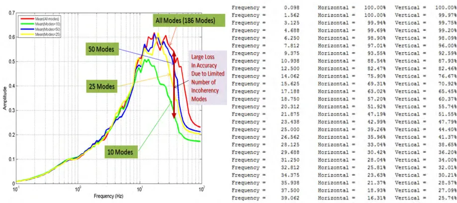
Figure 2 (left) shows the effect of using a limited number of incoherency spatial modes for computing the incoherent ISRS within a typical RB complex idealized by a complex FEA model, not a stick model with a infinite rigid basemat. As shown, the underestimation of the incoherent ISRS by using only 10 incoherency modes is up to a 50% in the high frequency range. Even for 50 incoherency modes, the ISRS are still highly underestimated.

A practical convergence criterion for the number of incoherency modes is to compute the percentage cumulative modal coherency contribution for a given number of modes. Such a criterion is similar to the cumulative modal mass criterion in structural dynamics. Thus, if the cumulative modal coherency contribution is above 90%, then, the number of incoherency modes included in the coherency matrix spectral factorization is sufficient. This criterion ensures that the free-field coherency matrix at the interaction nodes are accurately reproduced by the number of incoherency modes selected based on the convergence criterion.

rigid basemats, but as shown herein is far for being sufficient for realistic FEA SSI models with elastic basemats.

Figure 2 Effects of Using A Limited Number of Incoherency Modes to Compute ISRS.

Comparative ISRS for Different Number of Modes (left) and Cumulative Modal Contributions for 10 Incoherency Modes for A Typical RB Complex Footprint (right)

Effects of Incoherent Response Phasing

In practice, the SASSI type SSI analyses are performed for a set of selected SSI frequencies to compute the complex responses. The final complex responses for all Fourier frequencies, up to the cut-off frequency are then computed by using interpolation in complex frequency domain. As a result of such SSI methodology, the complex responses, both amplitude and phase components, are smoothed due to the interpolation in frequency domain. The smoothing effects are much larger for the incoherent motions than the coherent motions, since the incoherent motions include a significant random phasing component to capture the motion incoherency stochastic nature. Figure 3 shows that the smoothing effect of the complex response phase produced by the interpolation in the frequency domain for a number of 170 SSI frequencies instead of 4,096 Fourier frequencies. It should be noted that this smoothing effect reduces drastically the differential phases between neighboring frequency components.

Figure 3 Complex Response Phase Variation Within A Limited Frequency Band Between 8 Hz and 12 Hz for All 8,192 Fourier Frequencies (left plot) and 170 selected SSI Frequencies (right plot)

The EPRI approach phase smoothing is achieved by zeroing the phase in the SRSS approach, or by adjusting the phase in the AS and Simulation approaches (Short, Hardy, Mertz and Johnson, 2007). In both situations, the differential phases between closely-space frequency components are reduced to zero for SRSS or to a very small value for AS and Simulation with phase adjustment option. The result of the drastic reduction of the differential phases between neighbor frequency components produces an underestimation of the motion incoherency effects. The differential phasing between closely-spaced frequency components is a key modeling aspect of an accurate incoherent SSI analysis. The effects produced by differential phasing manifest are stronger for complex FEA models and less significant for stick models.

Figure 4 shows a comparison of ISRS results obtained for the EPRI AP1000 stick model sitting on a rock site. The incoherent SSI response was computed with and without complex response phase adjustment. The 5% damping ISRS plots are at the top of CIS. The ISRS plot comparison shows results for all 2,048 Fourier frequencies up to 50 Hz versus only 224 SSI frequencies with and without phase adjustment for different levels of phase smoothing, using a half-bandwidth equal to 10 and 50 Fourier frequencies, respectively. The upper plots are for without phase adjustment and the lower plots are for with phase adjustment. It should be noted that the phase adjustment for different smoothing levels affects only negligibly the ISRS results.

Figure 5 shows a ISRS comparison with and without phase adjustment for a RB complex FEA model with a footprint area of about 40,000 square ft. The RB complex is founded on a rock site. In contrast to the stick model results in Figure 2, for this FEA model the effect of the phase adjustment increases significantly the amplitude of the incoherent ISRS, especially in high frequency ranges. The green line that is well above the other lines is the for results with phase adjustment, while the other lines are for results without phase adjustment.

Figure 4 Comparative ISRS at Top of CIS Structure for 224 SSI Frequencies Without (upper plots) and With Phase Adjustment (lower plots) for Different Phase Smoothing and All Fourier Frequencies

Figure 5 5% Damping ISRS for X and Z Directions With (green) and Without Phase Adjustment (red, black, blue) and Different Smoothing Levels

Figure 6 5% Damping ISRS for Y and Z Directions Within the RB Complex FEA Model (with a 300 ft x

400 ft footprint area) for Coherent and Incoherent with 170 SSI Frequencies using SRSS With Zero Phase (10 modes) and Simulation With Phase Adjustment (10 samples) – EPRI-Validated Approach Solutions,

and Incoherent for All 5,700 Fourier Frequencies Using Simulation Without Phase Adjustment Solution (10 samples) – Theoretically Exact Solution

It should be noted that the “exact” incoherent ISRS results show large amplitude reductions starting from frequencies lower than 10 Hz. The ISRS reductions at frequencies below 10 Hz could be anticipated based on the 2007 Abrahamson rock coherence function variation around the 10 Hz frequency and the very large footprint area of the RB complex. However, if the EPRI-validated approaches are applied these ISRS reductions in low-mid frequency range below 10 Hz are totally invisible. It should be also noted that the larger the foundation size is, the larger the incoherency effects at mid and lower frequencies are. It is intuitive that for stiff foundations, the larger the foundation size is, the more sensitive its response to seismic waves with long wavelengths and low frequencies is. For the investigated RB complex with a very large footprint area, the effects of incoherency migrated down to 4-5 Hz frequencies.

EFFECTS OF BASEMAT FLEXIBILITY ON INCOHERENT SSI RESPONSE

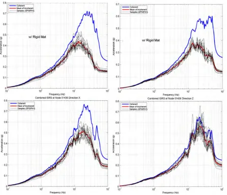
by 10,000 times. As shown the basemat flexibility amplifies the incoherent ISRS amplitudes by 25% for horizontal direction and about 80% for vertical direction. This indicates that is always rational to consider flexible mats in vertical direction (the out-of-plane direction).

Figure 7 Effects of Basemat Flexibility on Horizontal and Vertical ISRS; Rigid Mat (upper) and Elastic Mat (lower)

The incoherent motions produce differential soil motions underneath the foundation basemats. This implies that RB complex flexible baseslabs behave as multiple supported systems for which the input excitation motions at support points are not identical. Thus, for incoherent motions, as a result of differential displacement soil motions under baseslab, an increase of the baseslab bending moments is expected. Figure 8 shows the coherent and incoherent SSI displacements of a large-size baseslab, while Table 1 shows the bending moments in the baseslab for the two horizontal directions. It should be noted that the incoherent bending moments are about 30% to 130% larger than the coherent bending moments for the investigated case study. If the soil underneath the baseslab is stiffer then the incoherent bending moments increase. The relative stiffness between baseslab and soil subgrade is an important parameter.

could produce a large under evaluation of the elastic bending moments in the basemat. However, it should be noted that for the ultimate strength design approach used in the ASCE code for concrete design, the effects of the secondary stresses could be neglected if the baseslab has sufficient ductility to accommodate the SSI induced displacements.

Figure 8 Coherent and Incoherent SSI Displacements in Vertical Direction for a 350 ft Long Baseslab

Table 1: Baseslab Bending Moments for A Soil Deposit with Vs = 3,300 ft/s Zone # Coherent Incoherent Ratio Inc/Coh Coherent Incoherent Ratio Inc/Coh

MXX MXX MXX MYY MYY MYY

1 10.293 15.196 1.476 9.567 14.812 1.548

2 8.345 19.986 2.395 7.197 14.901 2.070

3 10.291 13.499 1.312 9.695 15.475 1.596

4 7.404 14.859 2.007 8.386 17.199 2.051

5 7.360 14.618 1.986 7.124 14.879 2.089

6 7.370 17.503 2.375 8.354 14.293 1.711

CONCLUSIONS

The paper shows that the EPRI validated incoherent SSI approaches provide always conservative SSI responses if the number of incoherency spatial modes considered in the analysis is sufficient. The zeroing of the complex response phases produces overly conservative ISRS for typical FEA SSI models.

The foundation flexibility increases the incoherent ISRS amplitudes and the bending moments in baseslabs. The relative stiffness between baseslab and soil subgrade is an important parameter.

REFERENCES

Ghiocel, D.M. (2013)“An Advanced Computational Software for 3D Dynamic Analyses Including Soil Structure Interaction”, ACS SASSI Version 2.3.0 Including Options A and FS Rev 1, Ghiocel Predictive Technologies, Inc., User Manuals, Installation Kit Revision 5, September 26

Short, S.A., G.S. Hardy, K.L. Merz, and J.J. Johnson (2007). “Validation of CLASSI and SASSI to Treat Seismic Wave Incoherence in SSI Analysis of Nuclear Power Plant Structures”, EPRI TR-1015111