A dynamic important methodology for the efficient estimation of rare event probabilities in regenerative simulations of queueing systems

A Dynamic Important Methodology

for the Efficient Estimation of Rare

Event Probabilities in Regenerative

Simulations of Queueing Systems

Michael Devetsikiotis

J.

Keith Townsend

Center for Communications

and

Signal Processing

Department Electrical

and

Computer Engineering

North Carolina State University

~

TR-91/14

Estimation of Rare Event Probabilities in Regenerative Simulations

of Queueing Systems

Michael Devetsikiotis _{J. Keith Townsend}

Center for Communications and Signal Processing,

Department of Electrical & Computer Engineering,

North Carolina State University, Raleigh, NC 27695-7914

Tel: (919)515-5200

Fax: (919)515-5523

Abstract

Importance sampling (IS) is recognized as a potentially powerful method for reducing sim-ulation runtimes when estimating the probabilities of rare events in communication systems using Monte Carlo simulation. When simulating networks of queues, regenerative techniques must be used in order to make the application of IS feasible and efficient. The application of regenerative techniques is also crucial in obtaining correct confidence intervals for the es-timates involved. However, using the most favorable IS settings very often makes the length of regeneration cycles infinite or impractically long. We present here a methodology that uses IS dynamically, within each regeneration cycle, in order to drive the system back to the regeneration state, after an accurate estimate has been obtained.

We also extend a technique we developed for finding near-optimal biasing parameters for link simulations to discrete-event simulations of queueing systems.

We demonstrate the combination of these techniquesby estimating blocking probabilities

for the

M/M/l/K, M/D/l/K,

and GI/D/I/K queues. Improvement factors of thirteen to

1

Introduction

Performance analysis of communications networks (e.g., asynchronous transfer mode, ATM)

requires the estimate of cell or packet loss probabilities. The (potentially) non-Poisson

statistics in these networks make pure analytical techniques difficult, and very low packet

loss probabilities (:::; 10-9 ) renders brute-force Monte Carlo simulation impractical. We

present in this paper a methodology which uses Importance Sampling (IS) to significantly

speedup simulations of queueing systems.

To obtain large improvement factors in simulation runtime using IS, the modification, or

bias of the underlying probability measures must be carefully chosen, else the runtimes may

increase. The most promising IS biasing schemes are parametric. In the case of bit error

rate estimation, increasing the noise variance

[1],

and more recently, translating (shifting)

the. distribution of the noise probability density function (pdf) have been used [2]. .The

translation biasing scheme resulted in large improvement factors. Similar results have been

obtained for single-sided pdf's using a scheme resembling translation or "quasi-translation"

[3,

4].

In the case of queueing networks, an exponential change of measure has been shown

to be optimal under certain conditions [5,6, 7].

Analytically minimizing the variance of the importance sampling estimator with respect

to the biasing parameters

[2,

8], or analytically finding the optimal exponential change of

measure [6, 7], has typically yielded results for systems which could be solved analytically

(e.g., linear system with additive Gaussian noise or simple queues with Poisson traffic).

Previously we have presented a technique for finding a near-optimal set of biasing parameters

for the translation and quasi-translation biasing schemes [3,

4].

Rather than use analytical

methods, the basic feature was that repetitive, very short simulation runs were used to

determine near-optimal translation values. Our method exploited a theoretically justifiable

relationship, for small sample sizes, between the probability estimate and the amount of

translation.

There are two significant contributions in this paper. First, we extend our method

simulation. Second, we present a method that uses IS dynamicallyin order to allow maximum

improvement while still maintaining an efficient regenerative evolution of the system. Using

optimal IS when simulating queueing systems virtually requires regenerative methods. Three

major advantages of using regenerative simulations are: Overcoming the deleterious effects

of system memory on the efficiency of IS, no need for a warm-up period, and improved

accuracy of confidence interval calculations [9].

An important issue we address in this paper is that near-optimal IS parameter settings

and regenerative simulation are in conflict - near-optimal IS parameter settings typically

re-sult in impractically long or even infinitely long (for systems with infinite queueing capacity)

regenerative cycles.

The idea behind dynamic IS is to use initially, in each regeneration cycle, the IS settings

that will lead to an accurate estimate with maximum efficiency and then change IS values

during the simulation so that the system will be driven to regeneration as quickly as possible.

This change occurs after the point of diminishing returns in efficiency of the IS estimate is

reached within a regenerative cycle. Thus the benefits of optimal IS and of short regeneration

periods are achieved simultaneously.

In contrast, when IS is used in the customary, static way, regeneration cycles will most

likely be impractically, or even infinitely long. Using static IS, the only techniques to

cir-cumvent this are either to force regeneration at chosen instants - which may not always be

theoretically correct, or choose IS parameter values under the constraint that regeneration

cycles be of manageable length - which may decrease the efficiency dramatically.

Section 2 gives a brief background of IS and regenerative techniques with respect to

esti-mating blocking probabilities in queueing systems. Our dynamic IS methodology is presented

in Section 3. Section 4 discusses the extension of our algorithm from

[3, 4]

to simulations

of queueing systems. Section 5 presents experimental results using a combination of our

dy-namic IS technique and our method of finding near-optimal IS parameter values, to estimate

the blocking probability of M/M/l/K, M/D /l/K, and GI/D /l/K systems. Improvement

factors in runtime over conventional Monte Carlo simulation from thirteen to fourteen

2

IS and Regenerative Simulations

2.1

Variance Reduction

Our goal is to estimate the expectation

E [V]

of a random variable (r. v. ) 1" that may in

general be a function of a random vector X, with a probability density function (pdf) px(x).

Then

E[Y]

=

J

ypx(x) dx

(1)

(2)

From a simulation standpoint, this would lead to the maximum likelihood empirical estimator

ElY]

=

1

E~l Yi which, depending on px(x) and }"(x), may require a very large number

of samples N to yield sufficient accuracy.

Under IS, we use a modified ("biased") version, Px(x), of px(x). Then, the expectation

E*[Y]

=

f

yw(x)Px(x) dx

is equal to E[Y] when w(x) == px(x)/Px(x), and Px(x)

:I

0 when Y ·px(x)

:I

o.

Therefore,

E[Y]

=

E·[Y] can be estimated by

(3)

where Px(x) is used in the simulation and N· samples are observed. The potential for

efficiency improvement offered by drawing samplesfrom Px(x) is indicated by the difference

between the variance (j2 of Y (under px) and (j~ of

y.

w(x) (under Px): ~(j2

=

(j2 - (j~

=

J

y2 (1 - w(x))px(x) dx. Clearly, if

w(x)

<

1 for all

x

such that Y(x)

1=

0 then ~(j2

>

o.

The key issue when using IS is the choice ofPx(x) - a good choice can lead to significant

improvement when compared to brute-force Monte Carlo, a poor choice can reduce the

efficiency of the simulation. Ideally, when Px(x) == l

r

(x )P.X(x)!

E[lr]

the variance under

Px becomes u~ ==

0

and ~O'2 == 0'2

[1].

However, this is merely a tautology since

E[l"]

is

the unknown quantity we need to estimate in the first place

[1, 10].

Moreover, in realistic

situations a closed-form expression for Y(x) is not known, neither is an explicit description

of the "important region", i.e., the region of the sample space that contributes to the integral

A more practical approach has been to choose

Px

(x) from a parametric family of

distri-butions, usually related to the original pdf. Variance modification

[1]

and translation

[2],

as

well as variations thereof

[11,

3,

4]

have been reported. Principles of large deviation theory

have also been applied [5], especially to Markov process and queueing systems simulation.

When Px(x) is chosen from a parametric family of distributions, the chief issue is

de-termining IS parameter values which yield good improvement. Analytical methods

[1, 2],

extrapolation techniques

[12, 13],

and numerical approximation

[7]

have been used with

vary-ing degrees of success. In this paper, we extend our statistically-based methodology [3, 4]

for choosing good IS parameter settings to queueing system simulation.

2.2

Est imat ion of Blocking Probabilities Using Regeneration

We discuss here how blocking probabilities can be estimated using regenerative methods

[9, 13].

We borrow most of the notation from

[14].

The analysis that follows is applicable to

a general GI/GI/l/K model.

The probability of blocking, P_{B ,} will be defined here as the probability of an arriving

customer being blocked (lost) after finding the queue already full. The empirical estimator

we will use is:

P

=

number of blocked a~rivals (i.e. "call congestion"). Let the simulated

B total number of arrIvals '

system include a single server and a single queue of length K-1,corresponding to a maximum

number in the system of K. Assume that discrete-event simulation is being used

[15]

and let

the events that drive the simulation belong to a finite set

E,

Let

V(tle)

denote the type of

event that occurred at instant

tie,

and let

{t

1 , •••

,tie, ... ,tN}

be the sequence of event epochs

observed in a simulation, with

V(tle)

E

E,

1 ~

k

~

N.

Let the number of customers in the

system just before the j-th event be Xj' Define the arrival indicator junction

It

as

A

{I,

j-th event is an arrival

Ij

=

_{0, otherwise}

and the blocked arrival indicator junction If as

It

= {

1, j-th event is an arrival that is blocked, .JYj

==

K

An event such that I!3

==

1 will be called hereafter an "important event" to distinguish it

J

from the ordinary events that drive the simulation. It is a crucial assumption that the system

displays regenerative behavior. That is, there exists a state that is visited infinitely often,

such that all new random events are scheduled independentlyof the past each time this state

is visited. We can then define stopping times B, and regenerative cycles (RC's) with length

L;

==

B, - Bi.:«. The important result that follows is that r.v.'s defined on disjoint RC's are

statistically independent and identically distributed (i.i.d.).

Let the number of blocked arrivals, after N events have been observed, be denoted by

nb

==

Ef::l

If.

If we break the summation over

L

disjoint sets of events, the number of

blocked arrivals in set i will be nb(i)

==

E~l

Ie,

where the second index, i, denotes set i,

M

i

is the number of events in set i and N

==

Ef=1

Mi. Then nb

==

Ef=l

nb(i). In a similar way,

we can group event epochs into disjoint sets {tIl" ..

,tIM

l } ,

{til, ... ,tiMi}' {tLI, ... ,tLML}'

with tIl ==

t

l and

tLML == tN·

In general, nbis a function of the sequence of event epochs

{t

l , . . . ,tN }: nb

==

g(tl , • · • ,tN ).

Thus E[nb]

==

J

N-fold··· I g(t

1 , ••• ,

tN) !T(t

1 , •. • ,

tN) dt

1 • · •

dtN,

where

!T(t

1 , ••• ,

tN)

is the

joint probability distribution (pdf) of the event processes. Using our summation over the

event sets E[nb] ==

Ef=l

IN-fold··' I g(t

1 , ••• ,

tiMi) fT(t

1 , • • . ,

tN) dt

1 •••

dtN,

since nb(i)will,

in general, be a function of all the events in its past, i.e., nb(i)

== g(

tl , . . . ,

tiMi)'

Now, if

we define the event sets as RC's, random variables defined in different RC's will be

statis-tically independent, yielding nb(i) ==

g(til, ... ,tiMi)' fT(tl, ... ,tN) ==

nf=l

fT(til,

,tiMi)'

and E[nb]

==

Ef=l

E[nb(i)]

==

Ef=l

IMi_fold···Ig(til, ... ,tiMi)!T(til, ... ,tiMi)dtil

dtiM

i ·

Under our assumption of independent generation of intervals between events

E[n,,]

==

Ef=l

I Mi-Jold · · · I g(til' · · · , tiMi)

n~l

!T( t jl) dtil · · · dtiMi·

Similarly, the total number of arrivals can be written as n_a == ""f:/_LJJ=1 I~_{J '} or as n_a ==

Ef=l

na(i),

where

na(i)

== E~l

Ij.

Since

na(i)

will be a function of

{til, ... ,tiAI.}, na(i)

==

q(til'.'"

tiMi)' it follows that, the expected number of arrivals will be given by E[n

a]

==

Ef=l

I

u, -

fold · · · I q(

til, · · · , tiMi)

n~l

!T( t

j1 )

dt

i 1 · • .

dt

i lt1i .

Using the regenerative method from [9], the blocking probability P_B can be expressed as

of arrivals in a RC ]. Then an estimator for P_B is given by -P_B =

~

=

it:

Ef:l

n,(i) where N_{4 1:;'}1 "£4_{L..Ji=1n 4}(')'₁

no (i),

nb(

i) are, respectively, the number of customers arrived and the number of customers

blocked, during the i-th RC. The numbers Lo and Lb of RC's observed for the estimation

of

fi"a

and

IV"

can, in general, be different. An accurate estimate of No, can be obtained

for single queue systems without using IS, since it does not involve the simulation of rare

events [14]. Estimates of No are thus obtained in separateruns without IS. From now on,

we restrict our attention to the efficient estimation of Ni:

Note that although

No

and

N;,

are statistically unbiased estimators of Noand N_{b ,} their

ratio yields a biasedestimate of PB (in general, E [X/Y]

#

E[X]/ E[Y]). However,

P;

is

strongly consistent and asymptotically unbiased [9]. Also from [9], we can calculate

asymp-totically valid confidence intervals for

P;,

which is one of the major motivations for using

regenerative methods.

2.3

Application of IS to Regenerative Simulation

Let the pdf for the random intervals T between events of type e E £ be given by p(T,

e).

In

applying IS, we will assume that the pdf's p(T,

e)

are modified separately to becomep*(T,

e),

for all e E £. The corresponding weight functions (equivalent to likelihood ratios) are defined

as W(T.·· e)

==

p('T'ij,e) for the j-th inter-event time in the i-th RC. Using the regenerative

11 , p. ('T'ij,e)

method, the expected number of blocked arrivals under the original event processes is

u,

E[nb(i)]

=

L!

18p(Til,V(il))",p(Tij,V(ij)) dTil ... dTij

(4)

;=1

where V(ik) returns the type of the event that occurred at instant k. Under the modified

processes (4) becomes

M·

E[nb(i)]

=

~

!

18p· (Til, V(

il)) · · ·

p. (Tij,

V(

ij))

W (Til,V(il)) · · ·l'V

(Tij,

V(

ij)) dTil · · · dTij

1=1

(5)

The empirical estimate for Nb resulting from (5) is

1 L" 1 L" Mi . ..

Nt,

== -

E

nb(i) == -

L L

li~

W

(Til,

V(d)) ... W

(Tij,V(~J))

L

b i=l

L

b i=1 ;=1

Since our simulation goal is to estimate the average number of blocked arrivals in aRC, Nb ,

and since blocked arrivals occur rarely under p(T,e),we should choose p. (T,e) such that the

frequency of blocked arrivals increases. Using IS, we generate inter-event times from p*(T,

e),

and "unbias" appropriately when we compute the estimate using the weight functions.

Clearly, in (6) above, the weight function for the event epoch tij depends on all random

inter-event times (e.g., interarrival or service times) previously drawn in the same RC. The

memory of the system is increasing within each RC. We use regenerative techniques to avoid

the deleterious effects of large system memory on the efficiency of IS.

3

A Dynamic IS Methodology: "Throttling"

3.1

Motivation

Discrete-event simulations of queueing systems can be modeled appropriately by a

general-ized semi-Markov process,as discussed in

[13].

The stateof the Markov chain involved can be

defined at the instants when simulation events occur, that is when arrivals, service

comple-tions or other events such as state changes in an arrival process occur. Regenerative cycles

(RC's) can then be defined as the periods between stopping times (instants that the system

visits the regenerative state) so that IS-related r.v.'s and estimates defined in different RC's

are statistically independent.

To illustrate, consider the following situation. Let the number of customers in the system,

at instant k be denoted by XIe, and assume that a regenerative state is chosen such that

X/e

=

O. Denote the utilization factor by p

=

AI

JL, where A is the arrival rate and JL the

service rate, and let p" be the utilization factor when IS is used. For the original system

(no IS), under light traffic conditions (e.g., p ~ 1.0) and with a low P_{B ,} it is clear that the

system is relatively empty most of the time, regeneration occurs rather often but blocked

arrivals are rare events.

Naturally, any IS modification of the probability measures involved should tend to make

"important events" (blocked arrivals) occur more often. This implies increasingthe effective

the issue of the frequency of occurrence of regenerative states under the modified measures.

We observe that, when IS settings are chosen so that the system traffic load is light (p.

<

1.0),

the system still visits X/e

=

0 although less often now, because of the higher utilization factor.

On the other hand, whenIS modifies the probability measures so that the system traffic load

becomes excessively large(p.

>

1.0)the average length of RC's, which is customarily at least

as long as the mean recurrence time of the condition X/e

==

0, grows to an impractical size.

As an example, the mean recurrence time Mo of X/e

==

0 would be infinite for practically

any GI/GI/l queue with p

2:

1.0(unstable system). Furthermore, for the M/M/1/K system

M« ==

O(pK), which clearly shows the exponential increase of M« when p

>

1.0. Other

queueing systems behave similarly, demonstrating the requirement for low p·'s, even when

"stability" is not an issue in its formal sense.

Clearly, unless restrictive assumptions on the traffic type allow regeneration to be forced

after the first blocked arrival (as in [6]), we are required to maintain at least moderate load

conditions, even under IS. This can limit dramatically the potential improvement that can

be realized with IS; analytical results for simple systems have shown that the optimal biasing

typically corresponds to p"

>

1.0[6], a fact that is supported by our empirical findings.

3.2

Dynarnic

application of

IS

To circumvent these difficulties, and combine IS and regenerative simulation we propose a

technique in which IS is implemented dynamically. Thus, IS parameter settings are varied

during each RC to initially allow important events[i.e., blocked arrivals) to occur frequently

then changed in a cycle to facilitate driving the system back to regeneration. Hence the idea

of "slowing down" or "throttling" the simulation after the high utilization IS settings have

been used long enough within a RC to yield accurate estimates, so that the regenerative

state will be reached, at which time the whole procedure will be repeated again. At the

beginning of a RC, a very high utilization factor is used (the search for optimal IS values

is further discussed in the next section) causing blocked arrivals to occur frequently. It

will be shown below that

nb(i)

in eq. (6) converges within each cycle (given enough time).

changed to now favor the re-occurrence of the regenerative state. That is, once the goal of

the first phase of the cycle (the phase we call "Efficient Estimation" or EE phase) has been

achieved, namely to observe enough important events (blocked arrivals), the second phase

(the "Accelerated Regeneration" or AR phase) regards the achievement of the regenerative

state as the important event and modifies the probability measures in order to accelerate the

return to such a state. In fact, as our experimental results also verify, the use of IS parameters

that speed-up the return to regenerative state, e.g. p" ~ p or p" ~ 1.0, for M/M/1/K,

M/D/l/K, or GI/D/I/K queues, can induce substantial runtime savings compared with

using the original, unmodified parameters in the AR phase of the RC.

3.3

Justification and Discussion

From the general IS formulation in (5) we can easily see that changing parameter values

during the simulation does not violate the basic IS rules, and as long as the appropriate

weight function is always used, the estimate obtained will be correct. Under the scheme

described in the previous part, the empirical estimate in (6) becomes

(7)

whereWk(Tik,e)= p~~.,.~••

eJ

explicitly denotes the dependence of the modified pdf's (and hence PJe or,Je,e

the weight function) on the instant k, reflecting the dynamic variation of the IS parameters.

During the EE phase of the RC, while a high utilization factor has been artificially

imposed due to IS and as the simulation progresses, the likelihood of the observed system

trajectory becomes smaller and smaller with respect to the trajectory under the unmodified

measures. Therefore, the weight function decreases within each RC since weights smaller

than 1.0 dominate, and the effect of successive important events on the cumulative estimate

decreases as well. Eventually, the weight function becomes so small that blocked arrivals

contribute insignificant amounts to the summation in (7). As Glynn and Iglehart show in [13],

in both the cases of a discrete-time Markov chain and the previously mentioned generalized

to zero (a.s.), as j - 00. It is straightforward to extend their approach to show that not

only Lj but also

P

Lj goes to zero (a.s.). It follows then, that ~~1L_j converges (a.s.),

and therefore also ~~1 Ii~ Lj converges a.s, as M; - 00. We can, therefore choose to

switch to the EE ("throttling") phase after the difference between the summation value at

two successive blocked arrival instants becomes smaller than a prespecified tolerance f. In

practice, this usually occurred only after 10 or 20 blocked arrivals had been collected. This

behavior has been consistently verified in our experimental observations.

4

Efficient IS Parameter Settings

In the context of bit error rate estimation for communication links [3,

4],

we proved that

when the method known as translation is used for biasing, and under certain conditions,

over-translation results in under-estimation of the expectation in

(2).

Over-translation means

shifting the pdf beyond the point of optimal IS improvement. In effect, we proved that, for

any fixed number of samples

N,

the estimate in (3), denoted here as

P(C),

goes to 0 almost

surely (a.s.) as the translation parameter Cgoes to infinity. At the other end (the lower end)

of the range of C, with C

=

0 corresponding to no IS biasing, the behavior of the simulation

will resemble closely that of brute-force

Me

simulation (i.e., no IS). Therefore, most of the

time no important events will occur in this region of operation. For the range of C-values

between these two extremes we note the following: As was demonstrated in

[4],

a robust

indicator for the performance of the IS parameter settings used, can be based on the sample

variance

V(C)

of the important weights (i.e., those that correspond to important events)

collected during the simulation. Such a performance measure is equivalent to an estimate of

the estimator variance lT~ discussed in Section 2. Furthermore, under the assumption that

the variance reduction induced by IS is a well-behaved function of the parameter C, the

local scatter

S[C)

of the estimate in a small neighborhood (C - iJ.C, C

+

iJ.C), compared

with such scatter elsewhere, can be thought of as a measure of the performance at C. We

concluded that, under certain assumptions, the estimates

pTC)

and

V(C),

plotted against

True

P

...-.

..

,...--.~

.

.

•

.

.1

...

.

,

:~ ~

~.

'.

'"

.,

I, •

.

.

.

.

,

.

,

.

_._....

IAl~lei

,~:;V

itA

J:

P(C)

,.-."

---ii

Variance

!

Estimate

,

c

C too low----tl.~1 C good IC too high ~

Figure 1: Probability Estimate P(C) and estimated sample variance

V(C)

vs. parameter C.

performance measure), combining the local scattermentioned above and the sample variance

estimate, was given in [4]. A near-optimal value for C can then be chosen as the value where

the composite cost function is minimum.

Extensive experimental results verified our theoretical observations and indicated that

large speedup factors over conventional Monte Carlo simulation could be achieved using

this method. Furthermore, we applied successfully the same method for locating favorable

IS settings, to a biasing scheme that resembled translation but was more appropriate for

single-sided pdf's ("pure" translation applied to single-sided pdf's violates IS rules and is

not permissible). This supported the expectation that our under-estimation theorem and IS

optimization algorithm could be extended to other IS schemes that involved more general

forms of uni-directional probability mass transfer (i.e., change of mean). Since inter-event

pdf's in discrete-event simulations are single-sided (time intervals are non-negative), such an

extension has particular practical significance.

Returning our attention to discrete-event simulations of queueing systems, let

p(

T,e) be

the pdf of the time

Te

between events of type e. Define Te as the expected value of

Te

and

lT~fI as its variance. The method of translation implies that the biased random intervals be

generated asT*

=

T

+

C,leading to p*( T,e)

=

p( T - C,

e),

with f;

=

fe

+

C and

u;:

=

u~

•.

A

2

and

cr;.

==

cr;. ·

C. In the case of the second biasing method, namely variance modification, it easily seen that there is indeed a probability mass transfer involved when

p(

r ;e)is single-sided

and C ~

o.

This is indicated by the fact that the mean of the biased pdf becomes

f:

=

s, ·

C.

Yet another biasing method is the "exponential twist" whereby p*(r,e)

==

eC"'p(r,e)IMe(C),

where Me (C) is the moment generating function of

Te

calculated at C [5]. The exponential

twist also generally involves probability mass transfer, and coincides with translation for a

Gaussian pdf or with variance modification for an exponential pdf.

Clearly, our observations concerning the behavior of

p(c), V(C),

and S(C) in link

simu-lations can be directly extended to the case of queueing simusimu-lations, by letting the densities

p(T,e) or their biased counterparts replace the noise densities, and the i.i.d. estimates nb(i)

in eq. (6) replace the i.i.d. observations (decisions) in link simulations. Empirical results

included in Section 5 further indicate that the above described method for selection of IS

settings, can be applied successfully to the simulation of queueing systems.

5

Experimental Results

In this section we use the techniques discussed earlier in this paper to estimate the average

probability of blocked arrival for

M/M/1/K, M/D /l/K,

and GIlD

/l/K

systems.

The M/M/l/K system had an average arrival rate A == 1.0, an average service rate

p,== 1.333, and a system capacityK = 101. The probability of an arrival being blocked could

be calculated analytically and was found to be 6.01x 10-1 4• For this system RC's coincided

with busy cycles. The average number of arrivals per RC was calculated analytically to be

No

=

4.0. As discussed earlier, we only needed to use IS to estimate the average number

blocked per RC, N". For this example, N"

=

2.41 X 10-13• and this is the number that we

estimated using our technique.

Under IS, the inter-arrival and service times were still exponential, but the rates .A and J.L

were independently multiplied by biasing parameters. Figure 2 shows a 3-dimensional plot

of the average blocked per RC for the M/M/1/K system. Each point on this plot represents

-14 ) Avg. Blocked / RC (True vatue - 2.41x 10

1000 RC'st Run

III10 -10 .a10 -II 'alO ·12 '1110-13 lalO ·I~ htO .

.,

1110 -us lalO -17

uio -II

hlO -19 20 30 ~ 50

Avg. InterArrivai Time Mull (x -0.02)

A=1.0,fJ.=1.333, K - 101, M/M/1/K

Figure 2: Plot of average number blocked per RC for an M/M/l/K queueing system as a

function of the IS parameters, namely average service time multiplier and average interarrival time multiplier.

IS parameters, namely service time multiplier, and interarrival time multiplier. The point

(0, 0) (front corner) corresponds to brute-force Monte Carlo. Note that this part of the plot

is not shown to provide a better view of the smooth region.

The opposite ends of the axes (near the 50) correspond to over-biasing of the probability

densities. Note that there is under-estimation of the average blocked per RC in the region

near these two extremes. The region of minimal local scatter (circled) corresponds to the

set of IS parameter settings which yield near-optimal improvement. The local smoothness

of this plot is indicative of small estimator variance.

Using our algorithm in [4], optimal parameter values are estimated to be 0.73 and 1.36 for

the interarrival time multiplier and service time multipliers respectively. Shown in Figures 3

and 4 are cuts of the 3-D figure through this optimal point. Also shown in these figures are

plots of the corresponding variance estimators. As discussed in [4], the algorithm minimizes

a cost function which combines the local scatter of the (estimated) average-blocked-per-RC

curve and the sample variance for each estimate. The effectiveness of the algorithm is clearly

1z10 -13

o 1z10-1 ..

a:

"'"

'i 1z10-1 5

~

1z10-1II

t

_{1.z10- 1 7}

1.z10-11

.

.

," .'1

i::

c • :::I I I opt

:j Ui -0.73

::

1.0

0.1

0.2

0.1 0.& 0." 0.2

Avg. InterArrfval T1me Multiplier

Figure 3: Cut of the 3-D plot of average blocked per RC overlaid with estimated sample variance, as a function of the interarrival time multiplier at the near-optimal value for the service time multiplier.

100 RC's I Run Avg.

InterAmval Time MultlpRer -0.75

0.8 1.0

•

as E

0.' •1ft

•

_S fi "C

0.4 _>

•

0.2

0.0 2.0 1 . ' 1.8

:"",:

~:::~. ~

.i

:...1

i...JI/

v

... 1.4 1.2

.

'.

'"

.

, "

\

..

:\..

~

I

1z1O -U a5 ~ 1z10-1• C

Avg. servtce Time Multiplier

Figure 4: Cut of the 3-D plot of average blocked per

RC

overlai~ with estimated s~mple v~ri­

These optimal IS parameter values were used in a set of longer simulation runs to estimate

the improvement over brute-force Monte Carlo simulation. For 100 runs with 1000 RC's per

run, the IS simulation estimate for Ni;

==

2.4 X 10-13• The 95% confidence coefficient for this

set of runs (1000 RC's per estimate) was calculated to be 2.89 X 10-15.

To estimate the improvement factor in simulation run time over brute-force MC, we used

the results in [16] to calculate the number of RC's required for a brute-force run to yield the

same confidence coefficient. Using this procedure we calculated an improvement factor of

4 x 1013

, i.e., our simulation estimated the average number blocked in a RC with a factor of

4 x 1013 _{fewer RC's than would have been required by brute-force Monte Carlo simulation.}

Note that this measure of comparison is based on the number of RC's, not the actual

simulation time that would have to include the length of RC's as well. Assuming the

com-putational effort required to complete the simulation of the i-th RC to be equal to its length

Li , the total runtime required to obtain an estimate based on NRC's is L = E~l Li, Then,

L

==

E{L}

=

N E{Li } . A fair comparison of simulation efficiency can then be based on

the time-reliability product

L

u~, where u~ is the variance of nb(i), the number of blocked customers during the i-th RC. In the case of brute-force MC, since the queue rarely fills up,

RC's are extremely short at the cost of a very large 0'2. Under favorable IS settings, the

length of RC's increases but u~ decreases so dramatically that the resulting time-reliability

product is orders of magnitude smaller than that of brute-force MC. The choice of

"throt-tling" parameters should make E{Li } as short as possible, without increasing (1'~. Hence,

while the purpose of the EE phase is mainly to make u~ low, the AR phase ensures that

regeneration will occur and keeps Li's short.

To see the effect of "throttling" on the simulation length, refer to Figure 5. In this figure,

which also corresponds to the same M/M/1/K system above, note that the leftmost point

corresponds to brute-force MC simulation. As we increase the amount of "throttling", the

RC length is shorter, as would be expected. The values of interarrival time multiplier and

service time multiplier shown on the rightmost point are the values used in all simulation

Note:

Run time becomes impractically longwhenoptimalISmultipliers of0.73and 1.36for arrivals and

departures respectively, areused

without "throttling"

4r---,----r---r--....--_

1 - - ---'-_...' - - _ . J - - _ - - '

1.22 1.0 0.01 5.0e-4 5.0e-7 5.0e-9 IS Setting after "Throttling" (x p)

!

3

tI

.§

~

&2r---t-t--+---J---~_..J

Figure 5: Plot of the average simulation run time in seconds versus the "throttling" (AR) parameters expressed as a fraction of the original utilization p. Runtimes are based on starting with the optimal IS settings and "throttling" after 20 lost customers, 100 RC's per run.

is biased for maximum improvement [i.e., the point (0.73, 1.36) from above). In this case,

RC's would be impractically long, as discussed earlier.

One other characteristic alluded to earlier was that as the trajectory in an RC evolves

under IS, L~1 Ii~

ru.,

Wk(Tik,

V(ik))

converges [a.s.) as

M

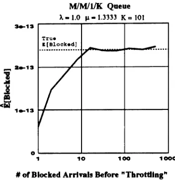
i increases. This can be seen in Figure 6, which shows the estimated number blocked per RC for the same M/M/1/K system

above as a function of the number of blocked arrivals observed in one RC before throttling.

After 10 to 20 blocked arrivals have been observed in an RC, the estimate has converged to

a desired level of precision.

The next example is an

M/D/l/K

queue, where A

=

1.0, the deterministic service rate is

fixed at 1.333, and the system capacity was K

=

59. Again for this system, RC's coincided

with busy cycles. Under IS, the inter-arrival times were still exponential, but the rate Awas

multiplied by a biasing parameter. A plot of the average blocked per RC and the sample

variance estimate as a function of the interarrival time multiplier is shown in Figure 7. As

before, the optimal IS biasing parameter value was estimated using our algorithm. It is

clear from Fig. 7 that the chosen value Copt

==

0.55 corresponds to the minimum scatter

MlM/lIKQueue

A- 1.0 Ji-1.3333 K=101

~13

True I.[BlookedJ

....~13 1---~~----+----1

!

j

!.

<CIII _{1~13 ...,..---10----+---1}

1000 100

10

O ' - - - ' - - - - . . . . A o - - - "

1

1#of Blocked Arrll'8ls Before "Throttling"

Figure 6: Plot of the estimated number blocked per RC as a function of the number of blocked arrivals observed before "throttling",

•

..

_E ~ o.tS :

•

~ 'i

0 •• >

0.2

1.0

0.8

0,0

... I

100 RC'sl Run • •, ..

:

·

_~

I::

~

I;:

_:l

~': :. :

':. .:..&.

:::_~ ::::~=:

I . ' • •:r....

,:

:

:iH::~

n

j:!ii

ii

~ ::::::::.

~ ~iii..=U il

.

" '

...

Hi!

;Avt- ...

ed/AC

I'

-.'

-I

i~I'

i

~~~.~

I : I

I,. ~ •

"'A~

~~t:l

....

. :

lx10-1 '" f - - _...._ - - . . - - _..._ - -...~0.0

1,0 0.5

Avg. InterArrival Time Multiplier

lxlO-1 3

1&10 -1.

1z10 -11

Figure 7: Plot of estimated average number lost per RC overlaid with estimated sample

1.0

0.8

i

.5 0.6 _i

! i

0.4 ·i_>

0.2

0.0

0.4 0 ..2

0.8 0.'

100 RC'. I Run

..·...···..···Uli

iU:

Hi

:==

'I,

'"

_{in::~ :}

i:' . niiii::

~'\" t M~J

i

j

:,'}¥

'f~ :;~:~, J

.,.., ':: l ., lz10-1•

+ - -..._~-...---.,---...O.0

1.0

lz10-15

Importance Bamplng Multlpler

Figure 8: Plot of estimated average number lost per RC overlaid with estimated sample variance, as a function of the multiplier m for an GIlD

I1/K

system.

case, we obtained an estimate of the average blocked per RC

N

b == 1.14 X 10-14.. The 95%

confidence coefficient for 100 runs at 1000 RC's per run was 4.46 x 10-16

• The improvement

over brute-force MC simulation was found to be 1.75 x 1014•

The last example we present is an GIlD

/l/K

queue, where Pr[interarrival time

=

al]

== p,

and Pr[interarrival time ==

a2]

== 1 - p, 0

<

P

<

1. In this example, at

=

2.1, a2 = 0.7,

p

==

0.6, the deterministic service rate is fixed at 1.25, and the system capacity is K == 19.

RC's coincided with busy cycles.

Under IS, p was multiplied by an IS multiplier m to obtain the biased distribution

Pr*[interarrival time at] == p*

==

pm, and Pr*[interarrival time

=

0:2]

== 1 - pm,

o

<

m

<

lip. A plot of the average blocked per RC and the sample variance estimate

as a function of the multiplier m is shown in Figure 8. The optimal IS biasing parameter

setting was found to be mopt

=

0.33. The estimate of the average blocked per RC, 95%

confidence coefficient, and improvement over brute-force l\IC simulation were found to be

6

Conclusions

We have presented a methodology that uses IS dynamically, within each regeneration cycle,

in order to drive the system back to the regeneration state, after an accurate estimate has

been obtained. Using this methodology, the benefits of optimal IS and of short regeneration periods can be achieved simultaneously.

We also extended a technique we developed for finding near-optimal biasing parameters

for link simulations to discrete-event simulations of queueing systems.

We demonstrated the combination of these techniques by estimating blocking

probabili-ties for the M/M/l/K, M/D /l/K, and GI/D /l/K queues. Improvement factors of thirteen

to fourteen orders of magnitude were obtained for these examples.

References

[1] K. S. Shanmugan and P. Balaban. A Modified Monte-Carlo Simulation Technique for

the Evaluation of Error Rate in Digital Communication Systems. IEEE Transactions

on Communications, COM-28(ll):1916-1924, November 1980.

[2] D. Lu and K. Yao. Improved Importance Sampling Technique for Efficient Simulation of

Digital Communication Systems. IEEE Journal on Selected Areas in Communications,

6(1), January 1988.

[3] M. Devetsikiotis and J. K. Townsend. A Useful and General Technique for Improving the

Efficiency of Monte Carlo Simulation of Digital Communication Systems. In Proceedings

of GLOBECOM '90, San Diego, CA, 1990.

[4] M. Devetsikiotis and J. K. Townsend. An Algorithmic Approach to the Optimization of

Importance Sampling Parameters in Digital Communication System Simulation.

Sub-mitted for publication in the IEEE Transactions on Communications.

[5] M. Cottrell, J .-C. Fort, and G. Malgouyres. Large Deviations and Rare Events in the

Study of Stochastic Algorithms. IEEE Transactions on A utomatic Control,

[6] S. Parekh and J. Walrand. A Quick Simulation Method for Excessive Backlogs in

Net-works of Queues. IEEE Transactions on Automatic Control, AC-34(1):54-66, January

1989.

[7] J. S. Sadowsky and J. A. Bucklew. On Large Deviation Theory and Asymptotically

Efficient Monte Carlo Estimation. IEEE Transactions on Information Theory,

IT-36(3):579-588, May 1990.

[8] R. J. Wolfe, M. C. Jeruchim, and P. M. Hahn. On Optimum and Suboptimum Biasing

Procedures for Importance Sampling in Communication Simulation. IEEE Transactions

on Communications, COM-38(5):639-647, May 1990.

[9] M. A. Crane and A. J. Lemoine. An Introduction to the Regenerative Method for

Sim-ulation A nalysis. Berlin: Springer-Verlag, 1977.

[10] Q. Wang and V. K. Bhargava. On the Application of Importance Sampling to BER

Estimation in the Simulation of Digital Communication Systems. IEEE Transactions

on Communications, COM-35(11):1231-1233, November 1987.

[11] H. J. Schlebusch. Nonlinear Importance Sampling Techniques for Efficient Simulation

of Communication Systems. In Proceedings of IEEE International Communications

Conference, ICC '90, 1990.

[12] W. W. LaRue and V. S. Frost. A Technique for Extrapolating the End-to-End

Per-formance of HDLC Links for a Range of Lost Packet Rates. IEEE Transactions on

Communications, COM-38( 4):461-466, April 1990.

[13] P. W. Glynn and D. L. Iglehart. Importance Sampling for Stochastic Simulations.

Management Science, 35:1367-1392, 1989.

[14] V. S. Frost and Q. Wang. Efficient Estimation of Cell Blocking Probability for ATM

Systems. In Proceedings of IEEE International Communications Conference, ICC '91,

[15] A. M. Law and W. D. Kelton. Simulation Modeling

&

Analysis. New York:

McGraw-Hill, 1991.

[16]

M. C. Jeruchim. Techniques for Estimating the Bit Error Rate in the Simulation of

Digital Communication Systems. IEEE Journal on Selected Areas in Communications,